Enhancing Magnetic Coupling Using Auxiliary Short-Circuited Coils

Abstract

The efficiency of Dynamic Inductive Power Transfer (DIPT) depends mainly on the coupling coefficient within the coupler. In order to improve this parameter, a novel approach has been introduced that results in a significant increase of between 25% and 36% at minimal additional cost in the case of juxtaposed rectangular coil configuration on the road. This method involves the incorporation of a passive additional short-circuit coil adjacent to the primary coil for obtaining a higher coupling coefficient, as has been theoretically demonstrated. Simulations carried out on Comsol have optimized the dimensions of this additional coil, not only for cost effectiveness and minimal space utilization, but also for optimal efficiency. Experimental validation was performed at reduced power, using a 2 kW test bench, and confirmed the estimation. The efficiency improvement proposed in this paper is crucial for improving the global DIPT efficiency and then facilitating its social acceptance.

1. Introduction

In response to climate change, electric vehicles have been developed to reduce global CO₂ emissions from the transportation sector [1]. However, challenges such as energy concentration, charging delays, cost of the vehicle integrating a battery and vehicle range limitations at charging stations have prompted the industry to explore Dynamic Inductive Power Transfer (DIPT) technology [2]. Indeed, this solution promises to reduce the embedded battery size, and then the cost of the electric vehicle and its weight; guarantee its autonomy; facilitate the battery’s load; and permit power electric dispatching. DIPT involves placing underground coils on the road to supply electricity to an embedded coil vehicle driving over, transferring energy without contact with the car. It has been under development worldwide for several years, with the goal of achieving global efficiencies of up to 90% [3]. Amongst the several topological options for the coil, a rectangular geometry has been selected as the best trade-off between efficiency and magnetic emission limitation [4]. Juxtaposition without any spacing is required for constant charging of the battery, and additionally for better efficiency, and for increasing the lifetime of the battery because of the limited number of charging cycles. However, this efficiency of DIPT is hindered by the poor coupling factor, resulting from the distance between the transmitter and receiver coils being at least 15 cm [5]. While a solution using a movable receiver to reduce this distance has been proposed, safety concerns have prevented industrial adoption. In addition, DIPT presents challenges such as electromagnetic compatibility (EMC) issues [6], regulatory compliance [7], life cycle assessment (LCA) determination [8], and the potential for the multi-power charging of trucks or buses [9], as well as thermal concerns [10] and the reliability of the inverter buried in the road [11] concerning the maintainability of the system. However, this work solely focuses on increasing the coupling factor for the position on the road to improve the efficiency of DIPT, although the solution can also be used for other fields of application.

The theoretical basis of our approach is demonstrated through equivalent schemes and equations, defining the coupling factor. Subsequently, Comsol simulations will be used to optimize the dimensions of additional short-circuit coils. These results will then be experimentally validated using a reduced-power 1.5kW system to prove the efficiency improvements of the proposal.

2. Theoretical Approach

In previous studies, it has been demonstrated that enhancing the magnetic coupling between the transmitter and receiver coils offers significant advantages. In the thesis published in [12], the author proposed placing auxiliary short-circuited coils next to the active transmitter coil to increase coupling between the transmitter and receiver coils. However, this proposition was validated only by testing without providing formal proof. This solution aligns well with the DIPT system considered, as multiple transmitters are already present. Therefore, enhanced magnetic coupling could be achieved without additional cost by utilizing existing transmitters as short-circuited coils next to the active transmitter (RSC). In addition, some other works have referred to coil addition for improving the performance with misalignments between primary and secondary [13,14], such as the proposed active shield for limiting the magnetic emission near the coupler [5].

In the following, a formal proof of this proposition is provided. This is conducted by presenting an equivalent reduced model, as shown in Figure 1. Then, the equivalent parameters could be found by identification with the two models. To simplify the demonstration, we assumed that the studied coils were lossless (no internal resistance and no magnetic losses).

The complete model can be described by the equations in Equation (1), while Equation (2) describes the reduced equivalent model. The original symmetrical model is

$$\left\{\begin{array}{c}\begin{array}{ccccccc}{\displaystyle \frac{U_1}{j\omega }}& =& L_1{I}_1& +& k_{\mathrm{1,2}}\sqrt{L_1{L}_2}{I}_2& +& k_{1,sc}\sqrt{L_1{L}_{sc}}{I}_{sc}\\ {\displaystyle \frac{U_2}{j\omega }}& =& k_{\mathrm{1,2}}\sqrt{L_1{L}_2}{I}_1& +& L_2{I}_2& +& k_{2,sc}\sqrt{L_2{L}_{sc}}{I}_{sc}\\ {\displaystyle \frac{U_{sc}}{j\omega }}& =& k_{1,sc}\sqrt{L_1{L}_{sc}}{I}_1& +& k_{2,sc}\sqrt{L_2{L}_{sc}}{I}_2& +& L_{sc}{I}_{sc}\end{array}\\ U_{sc}=-r_{sc}{I}_{sc}\end{array}\right.$$

(1)

$$\left\{\begin{array}{ccccc}{\displaystyle \frac{U_1}{j\omega }}& =& L_1^{\prime }{I}_1& +& k_{\mathrm{1,2}}^{\prime }\sqrt{L_1^{\prime }{L}_2^{\prime }}{I}_2\\ {\displaystyle \frac{U_2}{j\omega }}& =& k_{\mathrm{1,2}}^{\prime }\sqrt{L_1^{\prime }{L}_2^{\prime }}{I}_1& +& L_2^{\prime }{I}_2\end{array}\right.$$

(2)

By re-arranging Equation (1) and neglecting the short-circuit resistance ($r_{sc}$), we obtain the following relations (Equation (3)):

$$\left\{\begin{array}{c}\begin{array}{ccccc}{\displaystyle \frac{U_1}{j\omega }}& =& L_1\left(1-k_{1,sc}^2\right)I_1& +& \left(k_{\mathrm{1,2}}-k_{1,sc}{k}_{2,sc}\right)\sqrt{L_1{L}_2}{I}_2\\ {\displaystyle \frac{U_2}{j\omega }}& =& \left(k_{\mathrm{1,2}}-k_{1,sc}{k}_{2,sc}\right)\sqrt{L_1{L}_2}{I}_1& +& L_2\left(1-k_{2,sc}^2\right)I_2\end{array}\end{array}\right.$$

(3)

By comparing Equations (2) and (3), we can identify the equivalent parameters:

$$\left\{\begin{array}{c}{L}_1^{\prime }=L_1\left(1-k_{1,sc}^2\right)\\ L_2^{\prime }=L_2\left(1-k_{2,sc}^2\right)\\ k_{\mathrm{1,2}}^{\prime }={\displaystyle \frac{k_{\mathrm{1,2}}-k_{1,sc}{k}_{2,sc}}{\sqrt{\left(1-k_{1,sc}^2\right)\left(1-k_{2,sc}^2\right)}}} \\ M_{\mathrm{1,2}}^{\prime }=k_{\mathrm{1,2}}^{\prime }\sqrt{L_1^{\prime }{L}_2^{\prime }}=\left(k_{\mathrm{1,2}}-k_{1,sc}{k}_{2,sc}\right)\sqrt{L_1{L}_2}\end{array}\right.$$

(4)

From Equation (4), it is evident that the new equivalent inductances ($L_1^{\prime }$ and $L_2^{\prime }$) are consistently lower than the original ($L_1$ and $L_2$). However, the new equivalent mutual inductance ($M_{\mathrm{1,2}}^{\prime }$) could potentially increase, contingent on the sign of the product ($k_{1,sc}*k_{2,sc}$). This increase is achieved when Equation (5) is satisfied.

$$k_{1,sc}*k_{2,sc}<0$$

(5)

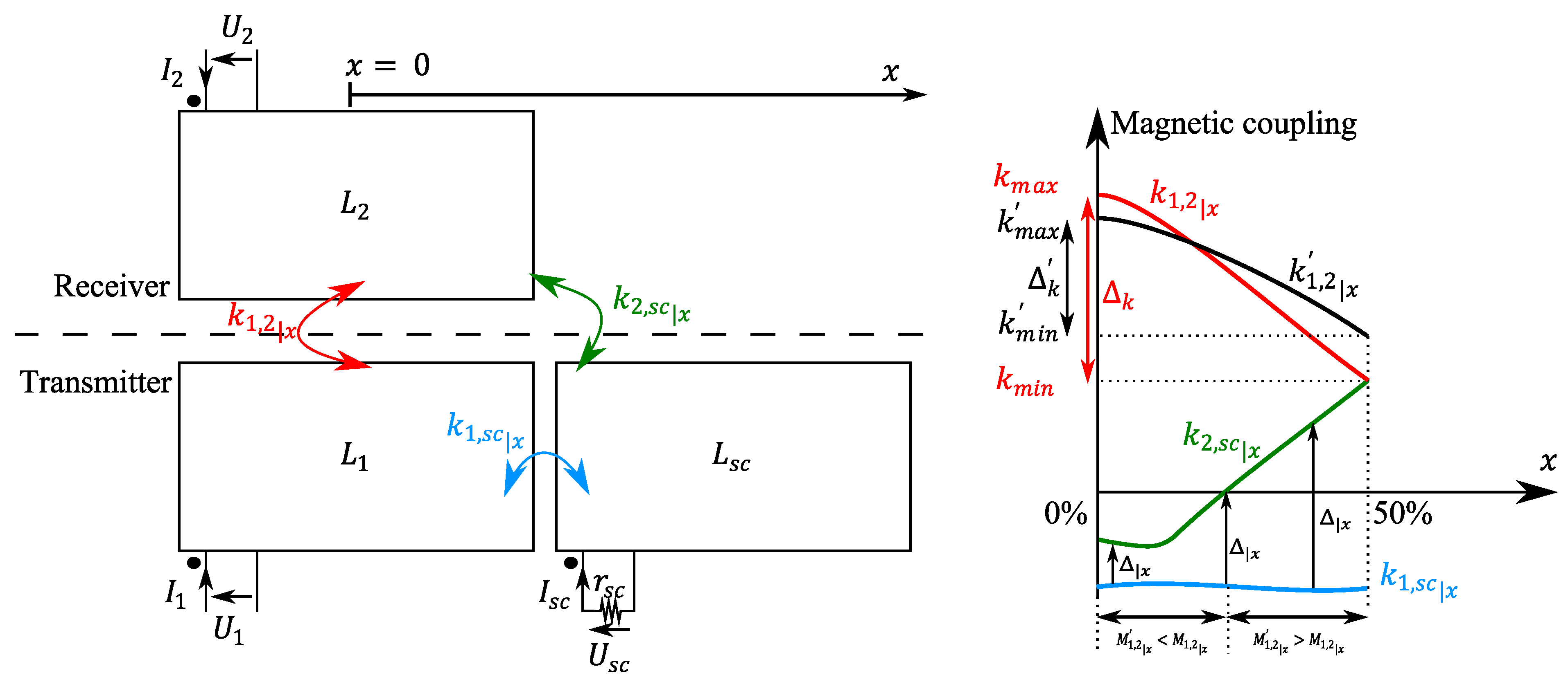
To clarify this point, we will consider a moving receiver ($L_2$) where ($x$) denotes its position, as shown in Figure 2. The zero reference of ($x$) is defined as the position at which the receiver ($L_2$) is centered above the transmitter ($L_1$). We will introduce (${∆}_{|x}$) as the following:

$${∆}_{|x}= {k_{2,sc}}_{|x}-{k_{1,sc}}_{|x}$$

(6)

We can then rewrite the expressions of Equation (4) in function $x$ as follows:

$$\left\{\begin{array}{c}\begin{array}{ccccc}{L_1^{\prime }}_{|x}& =& L_1\left(1-{k_{1,sc}}_{|x}^2\right)& & \\ {L_2^{\prime }}_{|x}& =& L_2\left(1-{k_{1,sc}}_{|x}^2\right)& -& L_2{∆}_{|x}\left(2{k_{1,sc}}_{|x}+{∆}_{|x}\right)\\ {k_{\mathrm{1,2}}^{\prime }}_{|x}& =& {\displaystyle \frac{{k_{\mathrm{1,2}}}_{|x}-{k_{1,sc}}_{|x}{k_{2,sc}}_{|x}}{\sqrt{\left(1-{k_{1,sc}}_{|x}^2\right)\left(1-{k_{2,sc}}_{|x}^2\right)}}} & & \\ {M_{\mathrm{1,2}}^{\prime }}_{|x}& =& {k_{\mathrm{1,2}}^{\prime }}_{|x}\sqrt{L_1^{\prime }{L}_2^{\prime }}& =& \left({k_{\mathrm{1,2}}}_{|x}-{k_{1,sc}}_{|x}{k_{2,sc}}_{|x}\right)\sqrt{L_1{L}_2}\end{array}\end{array}\right.$$

(7)

It is possible now to define the region as a function of the position ($x$), where the use of $L_{sc}$ in short-circuit will enhance the total equivalent mutual (${M_{\mathrm{1,2}}^{\prime }}_{|x}>{M_{\mathrm{1,2}}}_{|x}$). This enhancement is notable only when the magnetic coupling between the two transmitters is significant. Another benefit is the reduction in the new maximum coupling ($k_{max}^{\prime }<k_{max}$), leading to a smaller coupling variation (${∆}_k^{\prime }<{∆}_k$) since the new minimum coupling increases ($k_{min}^{\prime }>k_{min}$) over the range of the receiver’s motion ($0\%<x<50\%$). The typical order of magnitude with values based on two sets of parameters from $\left\{\begin{array}{c}{k_{\mathrm{1,2}}}_{|x=50\%}=15\%,;{k_{1,sc}}_{|x=50\%}=10\%; {k_{2,sc}}_{|x=50\%}=15\%\\ {k_{\mathrm{1,2}}}_{|x=50\%}=15\%,;{k_{1,sc}}_{|x=50\%}=15\%; {k_{2,sc}}_{|x=50\%}=15\%\end{array}\right.$ for $k_{min}^{\prime }$ would be around 12 to 18 % higher than the original $k_{min}$.

On the other hand, we observed a disadvantage arising from the de-tuning that occurs between the transmitter and receiver coil $\left({\displaystyle \frac{d{L_1^{\prime }}_{|x}}{dx}}\ne {\displaystyle \frac{d{L_2^{\prime }}_{|x}}{dx}}\right)$. This could have significant negative effects, particularly when performing fixed frequency control (current source mode). In this situation, the two resonant circuits become out of tune, contingent upon the value of ($x$).

By analyzing Figure 2, we can see that the origin of this de-tuning issue $\left({\displaystyle \frac{d{L_1^{\prime }}_{|x}}{dx}}\ne {\displaystyle \frac{d{L_2^{\prime }}_{|x}}{dx}}\right)$ arises from the spatial non-symmetry of the system. To address this issue, we propose a circuit, presented in Figure 3, which incorporates an additional short-circuited coil next to the receiver. The term “half-symmetrical” is used instead of “symmetrical” since the new proposed system could only possess symmetry over one diagonal and not full symmetry across the vertical axis, as we will see in a later proposition.

Using the same lossless approach as before, and neglecting the magnetic coupling between the two short-circuited coils (due to the large distance between them), we can determine the new equivalent model’s parameters:

$$\left\{\begin{array}{c}\begin{array}{c}{L}_1^{″}=L_1\left(1-k_{1,s{c}_1}^2-k_{1,s{c}_2}^2\right)\\ L_2^{″}=L_2\left(1-k_{2,s{c}_2}^2-k_{2,s{c}_1}^2\right)\\ k_{\mathrm{1,2}}^{″}={\displaystyle \frac{k_{\mathrm{1,2}}-k_{1,s{c}_1}{k}_{2,s{c}_1}-k_{1,s{c}_2}{k}_{2,s{c}_2}}{\sqrt{\left(1-k_{1,s{c}_1}^2-k_{1,s{c}_2}^2\right)\left(1-k_{2,s{c}_2}^2-k_{2,s{c}_1}^2\right)}}} \\ M_{\mathrm{1,2}}^{″}=k_{\mathrm{1,2}}^{″}\sqrt{L_1^{″}{L}_2^{″}}=\left(k_{\mathrm{1,2}}-k_{1,s{c}_1}{k}_{2,s{c}_1}-k_{1,s{c}_2}{k}_{2,s{c}_2}\right)\sqrt{L_1{L}_2}\end{array}\end{array}\right.$$

(8)

When using the half-symmetrical system, the following relations can be written:

$$\left\{\begin{array}{c}{k}_{1,s{c}_1}=k_{2,s{c}_2}=k_{\alpha }\\ k_{1,s{c}_2}=k_{2,s{c}_1}=k_{\beta }\end{array}\right.$$

(9)

Using the symmetry properties in Equation (9), we can simplify Equation (8) as follows:

$$\left\{\begin{array}{c}\begin{array}{c}{L}_1^{″}=L_1\left(1-k_{\alpha }^2-k_{\beta }^2\right)\\ L_2^{″}=L_2\left(1-k_{\alpha }^2-k_{\beta }^2\right)\\ k_{\mathrm{1,2}}^{″}={\displaystyle \frac{k_{\mathrm{1,2}}-2k_{\alpha }{k}_{\beta }}{\left(1-k_{\alpha }^2-k_{\beta }^2\right)}} \\ M_{\mathrm{1,2}}^{″}=k_{\mathrm{1,2}}^{″}\sqrt{L_1^{″}{L}_2^{″}}=\left(k_{\mathrm{1,2}}-2k_{\alpha }{k}_{\beta }\right)\sqrt{L_1{L}_2}\end{array}\end{array}\right.$$

(10)

As performed previously, the receiver’s displacement parameter ($x$) will be introduced. It is important to note that $L_2$ and $L_{s{c}_2}$ are locked together and move at the same rate. On the other hand, $L_1$ and $L_{s{c}_1}$ remain stationary.

Upon analyzing Equation (10), we can see that the de-tuning issue has been resolved with the half-symmetrical design. The variation in inductance as a function of the displacement ($\mathit{x}$) is now identical for both transmitter and receiver (${\displaystyle \frac{\mathit{d}{{\mathit{L}}_{\mathbf{1}}^{\mathbf{″}}}_{|\mathit{x}}}{\mathit{d}\mathit{x}}}={\displaystyle \frac{\mathit{d}{{\mathit{L}}_{\mathbf{2}}^{\mathbf{″}}}_{|\mathit{x}}}{\mathit{d}\mathit{x}}}$). Moreover, the coupling enhancement effect could potentially double with this solution (${\mathit{k}}_{\mathit{m}\mathit{i}\mathit{n}}^{\mathbf{″}}>{\mathit{k}}_{\mathit{m}\mathit{i}\mathit{n}}^{\mathbf{\prime }}>{\mathit{k}}_{\mathit{m}\mathit{i}\mathit{n}}$), or more than double, depending on the length of the transmitter coil as observed in Figure 4. The same effect can be observed in reducing coupling variations (${∆}_{\mathit{m}\mathit{i}\mathit{n}}^{\mathbf{″}}>{∆}_{\mathit{m}\mathit{i}\mathit{n}}^{\mathbf{\prime }}>{∆}_{\mathit{m}\mathit{i}\mathit{n}}$) over the displacement range of ($\mathbf{0}\%<\mathit{x}<\mathbf{50}\%$), which is really interesting in dynamic systems. Typically, the magnitude of ${\mathit{k}}_{\mathit{m}\mathit{i}\mathit{n}}^{\mathbf{″}}$ would be around 25 to 36 % higher than the original ${\mathit{k}}_{\mathit{m}\mathit{i}\mathit{n}}$.

3. Simulation Results

Comsol was employed to validate the theoretical approach proposed. We used unified copper wire on a ferrite plate to model the Transmitting (Tx) and Receiving (Rx) coils. The control configuration of the Tx coils is as follows: a Tx coil starts to emit when the Rx coil is positioned over it, covering at least 50% of its area. The considered distance between them is 150 mm. The coil in front of the Tx coil is set to short-circuit (Lsc1), while the previously emitting Tx coil is configured to be open-circuit (Loc1). Various sizes of additional short-circuit coil near the Rx coil (Lsc2) are simulated, whereas the original Rx and Tx coils are a square with 450 mm sides, as represented in Figure 5. This configuration corresponds to a 30 kW power transfer developed for industrial configuration [7]. The size of this additional coil is modified to obtain the best tradeoff between cost, spatial occupation, and mutual inductance.

The results of this latter parameter are illustrated in Figure 6, which presents the mutual between Tx and Rx for four cases in functions of the variation of the secondary position in x: the original one (red) without any additional coils, and with an additional short-circuit coil of the same size (green) and with its length reduced by a factor two (blue). We also considered the original case but with a variation in configuration on the Rx part, and called this solution RSC (magenta): the following coil is configured in short-circuit instead of open-circuit. We consider the starting point x = 0 mm as the optimal position, where the coils are perfectly aligned, resulting in the highest mutual inductance in all cases. Three main observations can be deduced about these results. Firstly, as demonstrated, the mutual inductance is higher when an auxiliary coil is present, with the most favorable case being 50% of the length. Indeed, for x = 0 mm, the mutual is lower but becomes superior as soon as there is a shift of x = 25 mm, until x = 250 mm for the 50% additional coil, and after x = 110 mm for the full additional coil. The energy gain depends on the car velocity and should be double due to the symmetry of the coupler. We can also consider a similar gain for a misalignment, as demonstrated theoretically. Secondly, the addition of an auxiliary coil of 100% reduces the inductance value of L2, subsequently reducing the measured mutual inductance between Tx and Rx. This behavior seems similar to that with a smaller coil, but as the mutual inductance level is smaller, the global mutual inductance is less impacted. Finally, the RSC solution reduces the mutual globally and is therefore not a viable solution for improving the coupler efficiency.

4. Experimental Validation

The results were validated by experimental approach for three cases: the reference, and with the addition of one full and one half-coil. A demonstrator with a full bridge and series capacity was constructed with a rectangular coil’s geometry of 450 × 450 mm². The clearance distance between Tx and Rx is approximately 150 mm, as shown in Figure 7. The coupling factor is measured by an impedance analyzer, Agilent 4294a, by the subtraction of the two inductances in series, and divided by 4 [15]. The mutual inductances between L1 and L2 are plotted in a function of x, beginning with the coils centered and shifting the moving coil with a step of 50 mm. We measured the system, when operating at 85 kHz, with only the coupler mutual, and hence after a capacity bank, as shown in Figure 7.

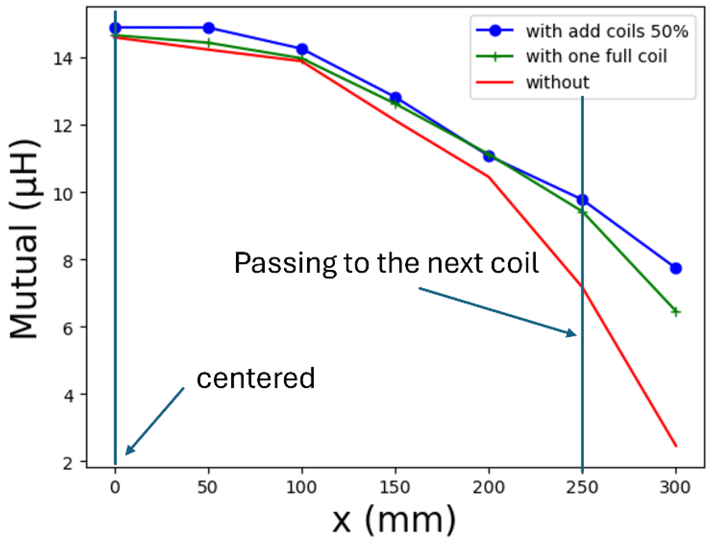
The results presented in Figure 8 show a strong coherence with the simulation and the theoretical approach. The lowest mutual is measured when the embedded coil passes through the next coil, at 250 mm. The mutual of the half short-circuit coil is then improved from 7 µH to 10 µH, and hence corresponds to the 25% improvement estimated in the theory. In addition, we measured the additional coil with six turns, and also for comparison with one single turn, and the difference was not relevant. However, when the secondary coil was set up slightly lower than in the model, reducing the mutual value a bit in comparison with the simulation, the results were almost similar, meaning that the short-circuit additional half coil requires a few turns to improve the mutual of the coupling system studied.

This result is validated experimentally on the 2 kW platform, as described in [16]. The following figures justify the efficiency improvement of the coupling coefficient for dynamical application, with the waveforms of the current and voltage of the coupler extracted from the scope and plot on Figure 9 for comparison, measured at the primary and the secondary coils without taking account of the resonant cell capacity. The coupling efficiency is for a similar voltage, the quotient of the output current divided by the input current considering the phases possible variations. Using the definition, we usually consider the quality factor Q, traducing the magnetic energy store (Lw) divided by the Joule effect (R), and the coupling coefficient can be as defined as

$$\mathrm{Q}={\displaystyle \frac{\mathrm{L}\mathsf{\omega }}{\mathrm{R}}}$$

(11)

$${\mathsf{\eta }}_{\mathrm{m}\mathrm{a}\mathrm{x}}={\displaystyle \frac{{\left(\mathrm{k}\mathrm{Q}\right)}^2}{{(1+\sqrt{1+{\left(\mathrm{k}\mathrm{Q}\right)}^2})}^2}}$$

(12)

As observed in Figure 9, when coils are centered with x = 0, the current is a bit higher than the one with the additional 50% coil, whereas the voltage is perfectly identical. With x displacement, the tendency will be for the contrary, as shown in Figure 10, with the coupler efficiency determination for 1.62 kW with an input signal of 45 V and 36 A. Whereas the voltage (blue and cyan) stays identical, the current (orange and yellow) varies in function of the displacement and the topology of the coil. The coupler efficiency is provided by the difference in active power, with a maximum at 90% when centering for the reference coupler, whereas we obtained only 88% for the proposed solution. For x = 15 mm, the difference is the opposite side, with a better efficiency with the additional coil of around 8% and reach of 10% when measured at its maximum for x = 200 mm. The current does indeed decrease faster without the additional coil, as demonstrated previously with the mutual determination.

5. Conclusions

The enhancements proposed theoretically in this study have been experimentally applied and validated, resulting in a considerable improvement to the power efficiency transfer for in-motion electrical vehicles equipped with an inductive power transfer system with only an additional short-circuit coil and also a specific control. The dimensions and placement of this additional coil were optimized using a Comsol simulation and then validated on a reduced power platform, a 1.5 kW prototype. The results show a 25% increase in the coupling factor when a vehicle is moving over, leading to enhanced power transfer efficiency and a reliability increase with less peak current in the coupler. Although a switch and more volume are necessary below the cars for this system, this paper proposed an original solution to save energy for the DIPT application.