An Exact Determinantal Calculus for Reliability and Reconfiguration of Radially Operated Distribution Networks

Abstract

A distribution feeder is built meshed and operated radially, so at any instant it occupies one of a combinatorial family of topologically radial configurations. We show that this family, weighted in the natural maximum-entropy way, is a determinantal point process whose kernel is the transfer-current matrix of the network, and we read that kernel in the operator’s language: the probability that a line section is energised equals its own self transfer-current factor, Foster’s sum rule is the trace identity, and the covariance of two switching states is minus the square of their normalised transfer current. Independent faults leave the feeder exactly within this family for any number of faults, whereas no restoration mechanism ignorant of the section resistances can return it there; among those that can, one is canonical, being the unique mechanism that reverses the fault, and its weight is the section’s transfer-current factor in the post-fault network with everything still energised shorted. We show, and report, that these weights are a structural diagnostic and not a repair priority. The maintained feeder is solved in closed form, and an exact transport equation prices what a reinforcement programme costs the feeder’s ability to reconfigure. The central spanning-tree and sector identities are verified against exhaustive enumeration; the dynamical and sensitivity statements are checked by exact master-equation computations and finite differences.

1. Introduction

1.1. The Problem a Utility Has

A medium-voltage distribution feeder is built meshed and operated radially. Tie switches between branches stand normally open so that the feeder remains radial, which simplifies protection coordination and fault isolation by avoiding closed-loop operating paths; at any instant exactly $N-1$ of the network’s line sections are energised and the rest stand open (Figure 1).

Three things then happen over the life of the feeder, and the utility has to answer a question about each. Sections fail: insulation ages, a trench is cut, a storm brings down a span, a fuse clears, and the feeder splits into islands, only one of which reaches the substation. Which restoration matters most, and how much of the feeder’s ability to reconfigure has been lost? Distributed generators fail: converters trip, protection operates upstream, units go out for maintenance. Which of them should be brought back first, when the crew cannot restore them all today? The feeder is reinforced: conductors are replaced and sections upsized over a multi-year programme. What does a reinforcement do to the feeder’s ability to reconfigure, and what does it cost the other sections?

None of these is a question about one configuration. Each is a question about the set of configurations the feeder can occupy, how large it is, how it is arranged, and how it degrades. This paper describes that set exactly.

1.2. Why the Existing Tools Do Not Answer Them

Reconfiguration of radial networks is a mature subject, and it is almost entirely an optimisation subject. The formulation goes back to Baran and Wu [1]; the literature since has produced branch-exchange heuristics, mixed-integer and convex programmes, radiality constraints in various encodings, metaheuristics and, recently, learning-based controllers, surveyed in [2,3]. What that literature computes is one configuration: the loss-minimising, or the load-balancing, or the most rapidly restoring one. Exhaustive search over the alternatives is routinely and correctly declared infeasible, because the number of admissible configurations grows multiplicatively with the number of tie sections; already at a dozen ties it is out of reach.

Two neighbouring literatures answer adjacent questions, and neither describes the family either. Service restoration after a fault is treated as a combinatorial search for a switching plan that reconnects the most-load subject to the operating constraints, surveyed in [4,5], with spanning-tree search among its tools [6]; it selects one post-fault configuration. Distribution reliability assessment [7,8] evaluates a given configuration from component failure and repair data and reports the customer-based indices standardised in [9], SAIFI, SAIDI and their relatives; it evaluates one configuration. The quantities of this paper are complementary to both: they are properties of the family, computed once from the resistances, and they feed rather than replace the restoration search and the index calculation (Section 9.3).

The consequence is that the space of admissible configurations is never described, only searched. A number of quantities a utility wants are properties of that space rather than of any point in it: how likely a given section is to be in service across the alternatives, which switching devices substitute for which, how many islands a maintained feeder carries on average, how much configurational freedom a reinforcement programme consumes. These are not obtainable from an optimised configuration, and they are not obtainable by enumeration either. Optimisation-based reconfiguration and analytical reliability assessment each work on one configuration at a time, and neither is meant to describe the family; the calculus of this paper describes the family and, in return, neither selects a configuration nor orders a repair. Section 9.3 sets the three side by side.

1.3. What the Resistive Description Decides, and What It Does Not

Everything below is computed on the resistive network: the conductances are $g_e=1/R_e$, and the quantities the construction delivers—effective resistances, current-division factors, Foster’s sum rule—are properties of that network. Section 2 explains why the resistive convention rather than the reactive one is the right choice for a distribution feeder, and Section 3 reports what changes under the alternatives.

This fixes a clean division of labour, and we state it at the outset so that no reader expects more. The kernel decides how much configurational freedom the feeder retains, which sections substitute for which, and how that freedom degrades under faults and under investment. Whether a given configuration is operable—voltages within limits, conductors within rating, protection still coordinated—is decided by load-flow analysis, and nothing here replaces it. The two are complementary and are meant to be run together.

1.4. What This Paper Does

The set of admissible radial configurations, weighted in the natural maximum-entropy way, is a determinantal point process [10,11,12] on the sections, and its kernel is the transfer-current matrix Y of the network. That single fact, classical in probability and to our knowledge not previously used in this setting, converts questions about a combinatorial family into determinants of a matrix computed once from one Laplacian pseudoinverse. On the benchmark feeder it replaces an enumeration of 50,751 configurations by a $37\times 37$ matrix; on a feeder with twenty ties it replaces a computation that cannot be performed at all.

A dictionary. The probability that a section is energised across the admissible configurations equals its own self transfer-current factor, $g_e{R}_{\mathrm{eff}}\left(e\right)$, the resistive-network analogue of a self power-transfer distribution factor and a quantity network analysis software already computes. Foster’s sum rule appears as the trace identity $\mathrm{tr}Y=N-1$ and serves as a structural check on the network data. The covariance of two switching states is minus the square of their normalised transfer current, so the kernel is a quantitative map of which devices substitute for which, and it exposes pairs, such as tie switches on different branches, that the single-line diagram does not suggest (Section 2).

An asymmetry between failure and repair. Independent random faults leave the surviving configuration exactly in the same determinantal family, with the same kernel, for any number of faults; the energisation profile is merely rescaled. Repair is different: no restoration mechanism chosen without knowledge of the section resistances can return the feeder to that family, not even one that knows the single-line diagram in full. Among the conductance-aware mechanisms that do, one is canonical: it is the unique kernel that reverses the random fault, and its weight has the closed electrical form $g_e{R}_{\mathrm{eff}}(e;G/B)$, the section’s own transfer-current factor in the post-fault network with everything still energised short-circuited. The weights sum to the number of islands minus one, which is a free consistency check (Section 4). We are explicit in Section 4 that upward intertwiners are not unique and that the canonical rule is singled out by time reversal alone.

A negative result we report rather than bury. It is tempting to read those weights as a repair priority. They are not. Measured against greedy service restoration on 250 fault episodes they recover load more slowly, and no faster than random order, because the kernel is built from a symmetric network with no distinguished node and therefore cannot know where the substation is. For deciding where to send a crew, a service-based ordering is correct and nothing here improves on it. The weights are a structural diagnostic, determining which restorations are unavoidable and which are redundant at the current step, and they define the canonical reversible repair model under which the finer statistics of the maintained feeder are exact (Section 4.8).

Closed-form reliability, and a robustness statement. Blind faults at rate $\gamma$ per energised section together with the canonical repair at rate $\beta$ per unit of vacant rank give a process whose law is the determinantal process with kernel $p\left(t\right)Y$ at every instant, with an explicit schedule $p\left(t\right)$. The expected number of islands is $1+(N-1)\gamma /(\beta +\gamma )$, the feeder is radially complete with probability $p^{N-1}$, and the model class is closed under independent thinning, so load-dependent indices are obtained by exact sampling with no burn-in. And the occupancy-based availability measures are robust to how the crew is dispatched: any repair policy with the same total rate leaves the occupancy process untouched (Section 5).

The same calculus on the generator fleet. Replacing the transfer-current kernel by the projection onto the generation modes estimated from output history, the restoration score of a failed distributed generator becomes the residual novelty of its retained-mode loading relative to the running fleet, and the scores sum to the number of uncovered generation regimes. Here the score is at least a quantity an operator might care about, unlike its network-layer counterpart; but the geometry is whitened and the score is not a gain in output variance, and we are explicit about what that does and does not license (Section 6).

An exact law for the slow layer. Along any schedule of conductances the kernel obeys $\dot{Y}=(I-Y)\Delta Y+Y\Delta (I-Y)$ with $\Delta$ one half the logarithmic rate of change in the conductances, so a reinforcement programme is fed in directly. The trace is conserved: reinforcement redistributes redundancy and cannot create it. The sensitivity is closed-form, and sizing driven purely by loading spends the feeder’s switching freedom; on the benchmark a redundancy term costing $1.7$ per cent in loss buys all of it back, a figure specific to that feeder and its loading (Section 7).

Research design. The study is calculus verified rather than a model fitted. Each result is stated with the level of assumption it needs, computed on one published benchmark whose data are given in full, and checked against an independent computation that does not use the result: exhaustive enumeration for the spanning-tree and sector laws, exact master equations for the dynamics, finite differences for the sensitivities, and paired simulation for the negative result on dispatch. No parameter is fitted. Everything above is exact for a frozen geometry and independent faults. The central spanning-tree and sector identities are verified independently against exhaustive enumeration of the 50,751 configurations of the benchmark feeder, at double-precision round-off (Section 3); the planning sensitivities are checked against finite differences, and the two-scale statement against an exact master-equation computation on a network with 194 partial configurations (Section 8). The results also differ in what they require of the feeder, and Section 10 sets out three levels explicitly: structural quantities assume nothing about how a configuration is chosen, occupancy indices need only independent faults, and the full configuration-level law needs the ensemble as an initial condition and a repair mechanism that intertwines adjacent sectors.

1.5. What Is Not New, and What We Do Not Claim

The transfer-current theorem is due to Burton and Pemantle [13] in the unweighted case and to Lyons [14] in the weighted form used here; Foster’s rule [15], the identification of commute times with effective resistances [16] and Wilson’s sampling algorithm [17,18] are classical, and the down-up operators of Section 8 belong to the theory of strongly Rayleigh measures [19,20,21,22,23,24]. Effective resistance and Kron reduction are themselves standard instruments of power-network analysis [25], and the total effective resistance has served as a global robustness measure of a network [26]; what those uses do not carry is the determinantal reading of the individual entries, which is what this paper exploits. The transport equation of Section 7 is the classical derivative of an orthogonal projection onto a moving subspace; what is new there is its instantiation by a conductance schedule and the consequences drawn from it. Equilibrium Glauber dynamics for determinantal processes were constructed by Shirai and Yoo [27] and others [28,29,30]; the projection boundary treated here is outside the scope of those constructions, because the L-ensemble matrix $K{(I-K)}^{-1}$ does not exist when the kernel is a projection.

We claim no difficulty. The results of this paper are an exact calculus rather than a hard theorem, and their value is that the identities are closed, cheap and checkable, not that they were troublesome to obtain. We also do not claim that a utility selects its configuration at random; Section 10 separates the results that depend on the ensemble from the ones that do not. Nor do we claim validation: all numerical results are computed on a published benchmark, specified in full in Appendix A, and comparison against an operating utility’s outage log remains the necessary next step.

1.6. Organisation

Section 2 sets up the feeder, the ensemble and the kernel. Section 3 verifies every identity used later against exhaustive enumeration. Section 4 treats faults and repair and establishes the asymmetry between them, together with the negative result on dispatch. Section 5 solves the maintained feeder in closed form. Section 6 carries the same calculus to a fleet of distributed generators. Section 7 gives the exact law of the kernel under a reinforcement programme. Section 8 couples the two time scales, Section 9 states what implementation costs, Section 10 sets out the limitations and Section 11 concludes. Appendix A gives all data and Appendix B the proofs not carried in the text.

2. The Feeder, Its Radial Configurations, and the Transfer-Current Kernel

2.1. The Feeder as an Electrical Graph

We model a medium-voltage distribution feeder as a finite connected graph $G=(V,E)$ with $N=\left|V\right|$ nodes and $m=\left|E\right|$ edges. Nodes are the substation bus together with the junction and load nodes; edges are line sections, each fitted with a switching device—a sectionaliser, a recloser, or a normally open tie switch. Line section e carries conductance $g_e=1/R_e>0$.

Fix an arbitrary orientation and let $B\in {\mathbb{R}}^{m\times N}$ be the signed incidence matrix, $G=\mathrm{diag}\left(g_e\right)$, and $L=B^{\top }GB$ the weighted Laplacian. For a connected feeder L has rank $N-1$ with kernel spanned by the all-ones vector, and $L^{+}$ is its Moore–Penrose pseudoinverse. The effective resistance [31] between nodes i and j is $R_{\mathrm{eff}}(i,j)={({\delta }_i-{\delta }_j)}^{\top }{L}^{+}({\delta }_i-{\delta }_j)$, and for an edge $e=\{i,j\}$ we write $R_{\mathrm{eff}}\left(e\right)$.

Distribution networks are built meshed but operated radially: with the tie switches normally open the feeder carries no closed operating path, which simplifies protection coordination and fault isolation. We note that radial topology does not by itself make fault current unidirectional once distributed generation is connected, and we make no such claim. A topologically radial configuration is therefore a spanning tree of G: exactly $N-1$ sections are energised, every node is served, and no loop is closed. We write $\mathcal{T}$ for the set of such configurations and call them admissible throughout. Whether a topologically radial configuration is also operationally feasible—voltages within limits, sections within rating, protection coordinated and selective, phases balanced, the switching permitted—is decided by load-flow analysis and lies outside this model (Section 10); “admissible” below always means topologically radial and never operationally feasible. This is the standard architecture of the reconfiguration literature, and it is the architecture the benchmark of Section 3 describes.

2.2. The Ensemble of Admissible Configurations

Rather than selecting one configuration, we describe the whole set $\mathcal{T}$ by a probability measure. For $\theta >0$ put

$${\mathrm{Pr}}_{\theta }\left[T\right]=\frac{1}{Z_{\theta }}\prod _{e\in T}{g}_e^{\theta },Z_{\theta }=\sum _{T\in \mathcal{T}}\prod _{e\in T}{g}_e^{\theta }.$$

(1)

Three remarks fix the status of (1), and we state them plainly because the ensemble is a modelling choice and not an operator’s objective.

First, (1) is the maximum-entropy law on $\mathcal{T}$ subject to a prescribed mean of the aggregate log-conductance ${\sum }_{e\in T}\log g_e$; $\theta$ is the associated Lagrange multiplier. It is the least committed description of the space of admissible configurations consistent with a given average electrical quality, and $\theta$ tunes how strongly the ensemble favours configurations built from the more conductive sections: $\theta \to 0$ gives the uniform law on radial configurations [32], $\theta \to \infty$ concentrates on the minimiser of ${\sum }_{e\in T}\log R_e$. This is a statement about aggregate log-conductance and not about physical loss: the loss of a configuration depends on the currents, hence on the loads and on the operating point, none of which the ensemble sees. The symbol $\theta$ is used for this exponent throughout and is not to be confused with the repair intensity $\beta$ of Section 5.

Second, the conductance is the resistive one, $g_e=1/R_e$, and this is a physical choice rather than a free one. The quantities the kernel delivers—effective resistances, current-division factors, Foster’s rule—are properties of the resistive network, and resistive loss is the quantity distribution reconfiguration has minimised since Baran and Wu [1]. The alternative convention $g_e=1/X_e$ belongs to the direct-current power-flow approximation, which is a transmission approximation: it presumes a small resistance-to-reactance ratio, whereas distribution feeders have $R/X$ of order one, which is why distribution analysis uses a full alternating-current solution or a branch-flow formulation rather than the linearised model. We therefore adopt $1/R$ throughout, report in Section 3 what the kernel looks like under $1/X$ and $1/\left|Z\right|$, and record in Section 10 that the ranking of candidates is sensitive to that choice, which is a reason to fix the convention on physical grounds, not a licence to vary it. The kernel is invariant under a common rescaling of all conductances, so the choice of units is immaterial; only the ratios matter.

Third, (1) is not a prediction of which configuration the operator will select. It is a description of the space in which that selection is made, and it is exactly this description that yields closed-form reliability indices, a canonical restoration mechanism and exact planning sensitivities, none of which is available from a single optimised configuration. Section 10 sets out the three levels at which the results below assert anything about a real feeder.

The normalisation is computable without enumeration: by Kirchhoff’s matrix-tree theorem [33] $Z_{\theta }$ is the determinant of the Laplacian built from $g_e^{\theta }$ with any one row and column deleted. To keep the notation light we absorb $\theta$ into the conductances and write g for $g^{\theta }$ from here on; every determinantal identity below holds for every $\theta >0$.

The electrical readings, however, do not. We take $\theta =1$ as the physical baseline of the paper: there Y is the transfer-current matrix of the actual resistive feeder and its entries are current-division factors of that feeder. For $\theta \ne 1$ the same determinantal identities hold, but they hold for the tempered ensemble, whose kernel is the transfer-current matrix of an auxiliary network with conductances $g_e^{\theta }$; ${\left(Y_{\theta }\right)}_{ee}=g_e^{\theta }{R}_{\mathrm{eff}}^{\left(\theta \right)}\left(e\right)$ is a current-division factor of that auxiliary network and not of the physical one. All numerical results below are at $\theta =1$ unless stated; the tempered family appears only as a sensitivity study, in Section 3 and Section 10.

2.3. The Transfer-Current Kernel

Set $M=G^{1/2}B$ and define the transfer-current kernel

$$Y=G^{1/2}B{L}^{+}{B}^{\top }{G}^{1/2}\in {\mathbb{R}}^{m\times m}.$$

(2)

Y is the orthogonal projection of ${\mathbb{R}}^E$ onto the space of rescaled stars $G^{1/2}\mathrm{ran}\left(B\right)$; in particular $Y=Y^{\top }=Y^2$ and $\mathrm{rank}Y=\mathrm{tr}Y=N-1$. Its entries have a direct electrical meaning. On the diagonal, $Y_{ee}$ is exactly the fraction of a unit current injected at one terminal of e and withdrawn at the other that flows through e itself. Off the diagonal, $Y_{ef}$ is the corresponding normalised transfer current: the symmetric normalisation of (2) means that the physical current in section f under that injection is $Y_{ef}\sqrt{g_f/g_e}$, the two coinciding when $e=f$. The normalisation is what makes Y a symmetric projection, and the determinantal identities below are statements about Y itself.

Theorem 1

(configuration ensemble is determinantal). For any distinct sections $e_1,\dots ,e_k$,

$$\mathrm{Pr}[e_1,\dots ,e_k\mathit{all}\mathit{energised}]=\det {\left(Y_{e_i{e}_j}\right)}_{i,j=1}^k.$$

(3)

This is the transfer-current theorem of Burton and Pemantle in the weighted form of Lyons [13,14,34]; we recall it because everything below rests on it, and we verify it by exhaustive enumeration in Section 3. Its content is that the $2^k$-dimensional joint law of any k switching devices is determined by the $k(k+1)/2$ numbers $Y_{e_i{e}_j}$, so questions about the operating ensemble reduce from combinatorics on $\mathcal{T}$ to linear algebra on Y.

2.4. What the Kernel Means to an Operator

Proposition 1.

Let $e=\{i,j\}$ be a line section. Then:

(i) 

$\mathrm{Pr}\left[e\mathrm{energised}\right]=Y_{ee}=g_e{R}_{\mathrm{eff}}\left(e\right)$, which is exactly the fraction of a unit current injected at i and withdrawn at j that flows through e itself; we call this the section’s self transfer-current factor;

(ii) 

${\sum }_{e\in E}{g}_e{R}_{\mathrm{eff}}\left(e\right)=N-1$ for every network and every choice of conductances;

(iii) 

for $e\ne f$, $\mathrm{Cov}(\mathbf{1}\left\{e\right\},\mathbf{1}\left\{f\right\})=-Y_{ef}^2\le 0$;

(iv) 

$Y_{ee}=1$ if and only if e is a bridge of G; $Y_{ee}=0$ is impossible for $e\in E$.

Proof. 

(i) is (3) at $k=1$ with ${\delta }_e^{\top }{G}^{1/2}B{L}^{+}{B}^{\top }{G}^{1/2}{\delta }_e=g_e{R}_{\mathrm{eff}}\left(e\right)$, together with the current interpretation of $Y_{ee}$. (ii) is $\mathrm{tr}Y=\mathrm{rank}Y=N-1$. (iii) is (3) at $k=2$. (iv) A projection has diagonal entries in $[0,1]$, with $Y_{ee}=1$ exactly when the corresponding coordinate vector lies in the range, which happens precisely for bridges; and $Y_{ee}=g_e{R}_{\mathrm{eff}}\left(e\right)>0$ for every present edge.    □

Part (i) is the resistive-network analogue of a self power-transfer distribution factor, computed by the same linear algebra; we avoid the term PTDF itself because in power-system usage [35] it denotes the incremental change of a branch real-power flow under a specified source–sink power transfer, a related but not identical object. Part (ii) is Foster’s rule [15]: the sum of all self transfer-current factors equals the number of nodes minus one, and a violation indicates an error in the network data rather than an unusual feeder. Part (iii) says that no two sections are positively correlated, so the matrix $(Y_{ef}^2)$ is a quantitative map of which switching devices compete with which (Figure 2).

Remark 1.

Part (i) is the practical bridge of this paper. The probability that a section is energised in a random admissible configuration is not a new quantity to be estimated but a current-division factor already available in network analysis software. Everything that follows is expressed in these terms.

In engineering terms, the kernel is assembled from one factorisation of the network Laplacian, which any load-flow or short-circuit program already performs. Its diagonal is a current-division factor: the share of a unit current between the terminals of a section that the section itself carries, the remainder flowing round through the meshes. Its off-diagonal entries, squared, say how strongly two switching devices compete for a place in the radial configuration. Its trace, which must equal the number of nodes minus one, is a check on the network data. Nothing beyond these four readings is needed to use Proposition 1;

Table 1. Dictionary between network terminology and the quantities of the kernel.

Feeder Term	Model Quantity
line section	edge e
switching state	indicator $\mathbf{1}\{e\in T\}$
radial configuration	spanning tree T
section with no bypass	bridge; $Y_{ee}=1$
self transfer-current factor (current-division factor)	$Y_{ee}=g_e{R}_{\mathrm{eff}}\left(e\right)$
normalised transfer current between two sections	$Y_{ef}$; the physical current is $Y_{ef}\sqrt{g_f/g_e}$
substitutability of two devices	$-Y_{ef}^2$
number of islands	$N-\left|B\right|$
sections still to re-energise	vacant rank $r-k$

collects the correspondence.

Remark 2.

$Y_{ee}$ also equals half the product of the equilibrium current across e and the commute time of the associated network random walk between its terminals [16,36]. We record the identity because it explains why heavily used but electrically remote sections are the ones the ensemble insists on; it is not used in the sequel.

Figure 2. (a) Probability that each section is energised. (b) The map of normalised transfer currents $|Y_{ef}|$, read as the substitution map between switching devices; squares mark the competing pairs of Table 2.

Figure 2. (a) Probability that each section is energised. (b) The map of normalised transfer currents $|Y_{ef}|$, read as the substitution map between switching devices; squares mark the competing pairs of Table 2.

Table 2. The strongest substitution relations between switching devices.

Section	Section	Normalised Transfer Current $|{\mathit{Y}}_{\mathit{ef}}|$	Covariance
L12	T2	0.2495	−0.0622
T1	T3	0.2211	−0.0489
L19	T1	0.2025	−0.0410
L21	T3	0.2006	−0.0402
L08	T3	0.1933	−0.0374
L09	T2	0.1802	−0.0325

Table 2. The strongest substitution relations between switching devices.

Section	Section	Normalised Transfer Current $|{\mathit{Y}}_{\mathit{ef}}|$	Covariance
L12	T2	0.2495	−0.0622
T1	T3	0.2211	−0.0489
L19	T1	0.2025	−0.0410
L21	T3	0.2006	−0.0402
L08	T3	0.1933	−0.0374
L09	T2	0.1802	−0.0325

2.5. Computational Cost

Forming Y costs one pseudoinverse of an $N\times N$ Laplacian, $O\left(N^3\right)$, after which every statement below is a determinant of size at most a few. For the benchmark feeder this replaces an enumeration of 50,751 admissible configurations by a single $37\times 37$ matrix; for feeders with twenty or more tie sections enumeration is out of reach altogether while the kernel is obtained at the same cost.

3. Verification on a Benchmark Feeder

The central spanning-tree and sector identities used in Section 4, Section 5, Section 6 and Section 7 concern finite objects and can be independently checked by exhaustive enumeration on a feeder small enough to enumerate. We do this once, here, before the statements are used, so that the reader may take the remaining sections as computation rather than as assertion; the planning sensitivity is checked against finite differences and the dynamical statements by exact master-equation computation, the latter in Section 8.

3.1. The Benchmark Feeder

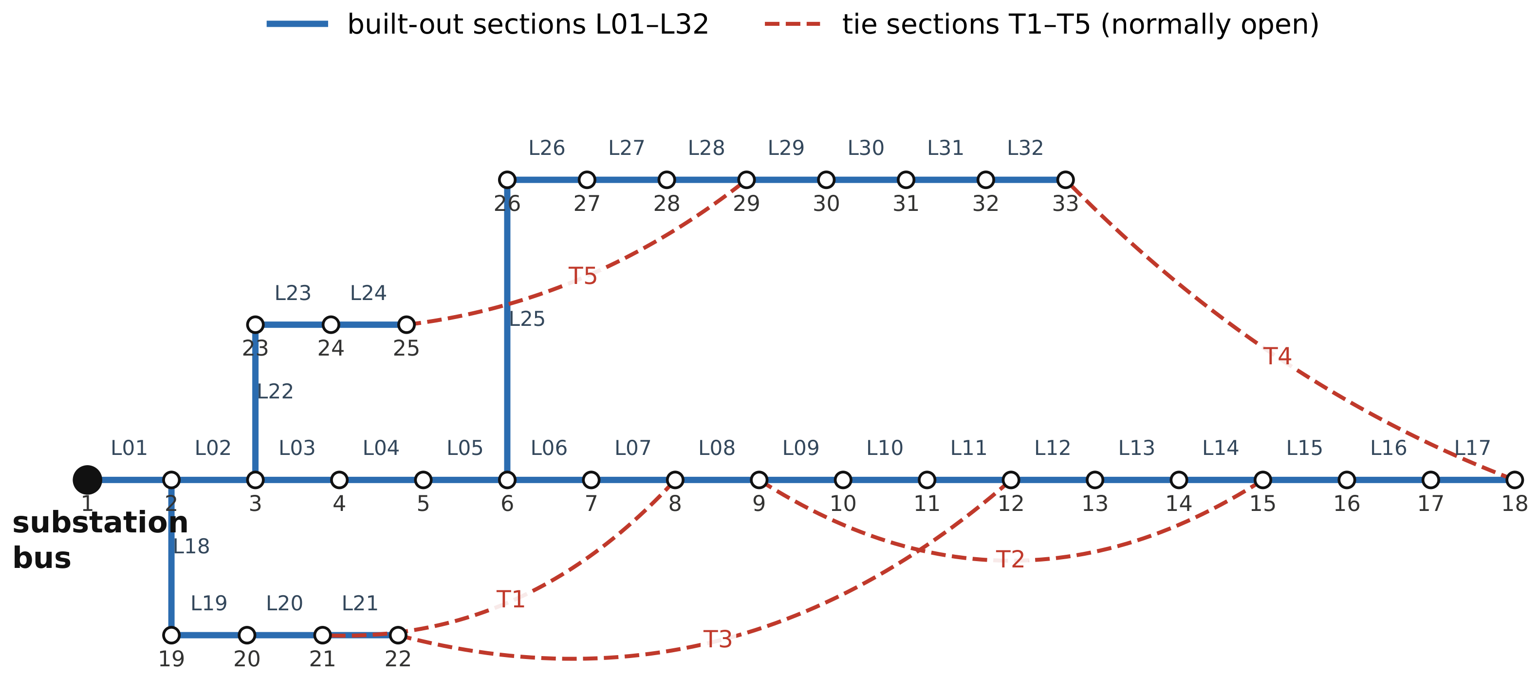
The benchmark has $N=33$ nodes and $m=37$ line sections: 32 forming the built-out branches and 5 tie sections, normally open, joining branches to one another. It is the standard 33-node distribution test system of Baran and Wu [1], used here with its own published resistances; the complete section list is given in Appendix A. The head section leaves the substation bus, which has a degree of one, so that section is the only bridge; the remaining 36 sections each lie on at least one loop and are therefore switchable.

We use a published benchmark deliberately. The purpose of this section is verification of exact identities, for which a fully specified and reproducible network is worth more than a proprietary one; validation against measured outage data is a separate task, noted among the limitations in Section 10.

3.2. Enumeration of Admissible Configurations

Exhaustive search over the ways of leaving five sections open, retaining those whose complement is connected and spanning, yields $|\mathcal{T}|=\mathrm{50,751}$. As an independent check of both the topology and the enumeration code, Kirchhoff’s matrix-tree theorem applied to the weighted Laplacian gives the same weighted total to ten significant digits, and the unweighted determinant returns 50,751 exactly.

This network is close to the practical ceiling for enumeration: with five independent loops the search is instantaneous, but the count grows multiplicatively with the number of tie sections. That asymmetry is the point of the paper: Y is a single $37\times 37$ matrix obtained from one pseudoinverse, and its cost does not grow combinatorially with the number of loops.

3.3. The Kernel

Assembling Y gives a matrix symmetric and idempotent to machine precision, of rank 32, with $\mathrm{tr}Y=32.0000000000=N-1$, which is Proposition 1(ii). Exactly one diagonal entry equals one, the head section, confirming Proposition 1(iv).

Table 3. The six sections whose energisation is least certain across the admissible configurations.

Section	Nodes	$\mathrm{Pr}\left[\mathbf{Energised}\right]$
T1	8–21	0.5453
T2	9–15	0.5801
T3	12–22	0.6631
L12	12–13	0.7224
L19	19–20	0.7373
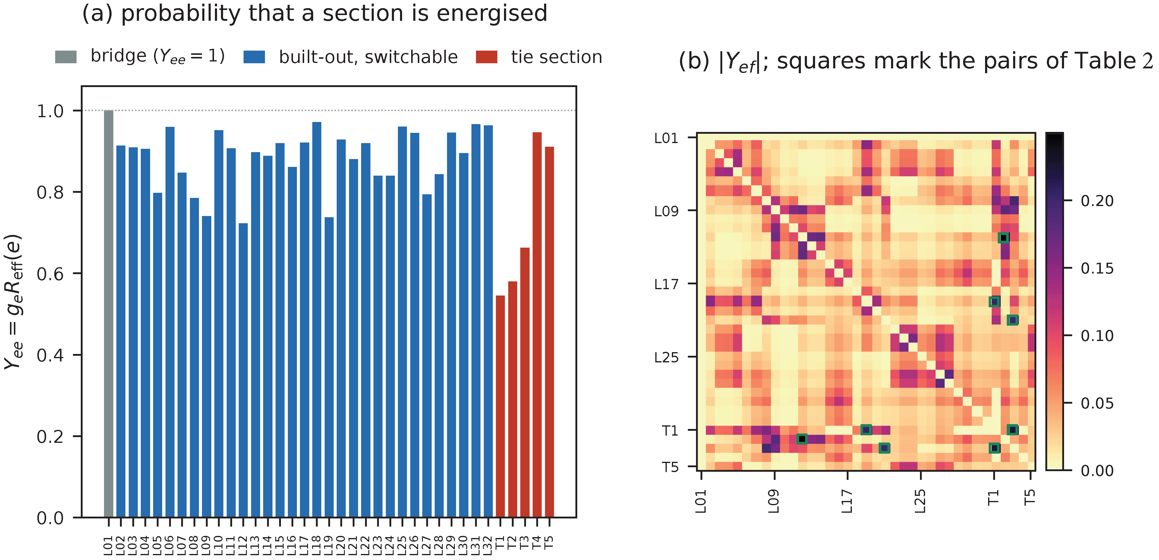
L09	9–10	0.7408

lists the six sections whose energisation is least certain.

The second entry of Table 2 deserves comment: T1 and T3 are two distinct tie sections, on different branches, that compete with one another more strongly than either competes with its own neighbours. Such pairs are not apparent from the single-line diagram and are exactly what the kernel is for.

3.4. The Determinantal Law

Table 4. Verification of the determinantal law against exhaustive enumeration of 50,751 configurations.

k	Subsets Tested	Max. Error
1	all 37 sections	1.4 × ${10}^{-15}$
2	all 666 pairs	2.6 × ${10}^{-15}$
3	400 random subsets	3.0 × ${10}^{-15}$
4	400 random subsets	3.0 × ${10}^{-15}$
5	400 random subsets	2.9 × ${10}^{-15}$
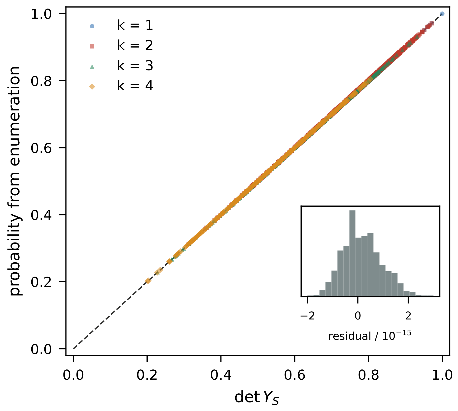
8	400 random subsets	2.3 × ${10}^{-15}$

compares the enumerated probability that a set of sections is energised with the determinant of (3) for subsets of up to eight sections.

All discrepancies are at the level of double-precision round-off (Figure 3). We stress that this is a genuine check and not a tautology: the left-hand side is a combinatorial sum over 50,751 enumerated configurations and the right-hand side is a determinant of a matrix built from a pseudoinverse; the two computations share no code path.

3.5. The Electrical Readings, the Sector Family and the Restoration Weights

Computing $g_e{R}_{\mathrm{eff}}\left(e\right)$ from the Laplacian pseudoinverse, and separately computing the self transfer-current factor of each section by injecting a unit current at its terminals, reproduces the diagonal of Y with maximum discrepancy $8.1\times {10}^{-15}$. The equivalent form $Y_{ee}=\frac{1}{2}{J}_e{C}_e$, with $J_e$ the equilibrium current share across the section and $C_e$ the commute time between its terminals, agrees to the same precision, and ${\sum }_e{J}_e{C}_e=64.000000=2(N-1)$.

De-energising one uniformly chosen section of a configuration drawn from the ensemble and computing the exact resulting law over 31-section forests reproduces ${\mu }_{r-1}$ of (4) with a maximum relative error of $8.0\times {10}^{-15}$; two independent faults reproduce ${\mu }_{r-2}$ to the same precision. For partial configurations with $k=20,25,28,30,31$ energised sections both sides of (5) agree to $4.9\times {10}^{-15}$, and the consistency check of Corollary 1 holds to $1.1\times {10}^{-14}$. A quantity defined through the determinantal ensemble is thus computed correctly by a purely electrical procedure that involves no probability at all.

Increasing the conductance of a section and recomputing the kernel by finite differences reproduces Corollary 6 with maximum error $2.0\times {10}^{-9}$ at a step of ${10}^{-6}$, and the sum of the predicted changes over all sections vanishes to $4.8\times {10}^{-16}$.

3.6. Robustness to the Weighting Convention

Replacing $g_e=1/R_e$ by $1/X_e$, the convention of the direct-current power-flow approximation, leaves $\mathrm{tr}Y=32$ and changes the entries modestly: the least certain section is still T1, with probability $0.5110$ instead of $0.5453$; $1/|Z_e|$ gives $0.5351$. Section 2 explains why $1/R$ is the convention we adopt and Section 10 records how far the ranking moves under the others. 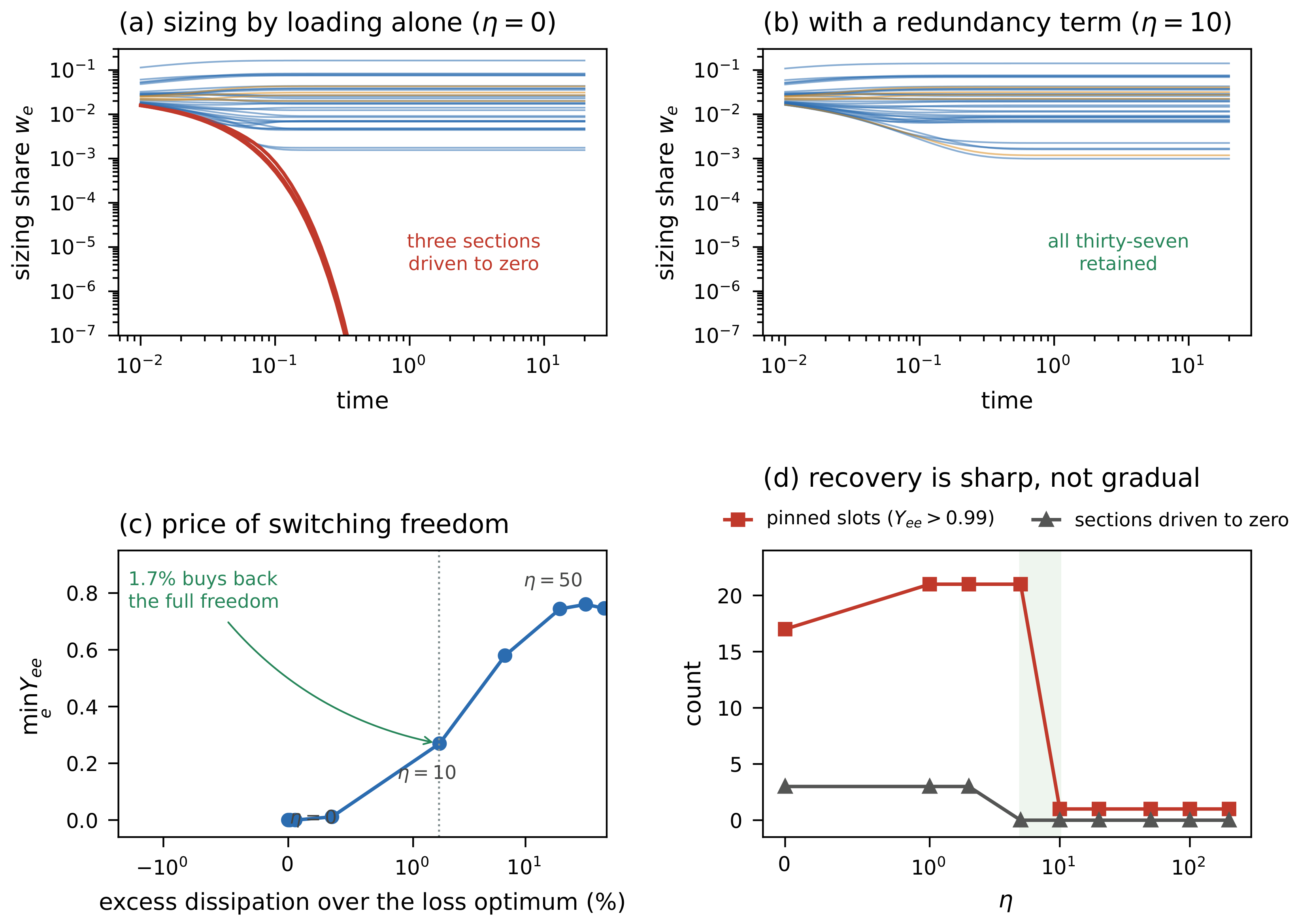Raising the conductances to a power $\theta$ as in (1) tightens the ensemble as expected: the smallest diagonal entry falls from $0.6466$ at $\theta =0.5$ to $0.5453$, $0.3844$ and $0.1656$ at $\theta =1,2,4$, while the number of sections energised in essentially every configuration rises from 1 to 4 and then to 16. The parameter $\theta$ therefore controls how much switching freedom the ensemble ascribes to the feeder, and the identities hold along the whole family.

The central spanning-tree and sector identities have thus been verified against exhaustive enumeration of 50,751 configurations, with discrepancies at double-precision round-off; the planning sensitivity was checked against finite differences here, and the dynamical statements are checked separately, by exact master-equation computation, in Section 8. From this point on we use the kernel and dispense with enumeration, which for feeders of realistic size is not merely expensive but impossible.

4. Random Outages and the Restoration Order

4.1. Partially Energised Feeders

A sequence of faults leaves the feeder with fewer than $N-1$ energised sections. Write $r=N-1$ and, for $0\le k\le r$, let ${\mathcal{I}}_k=\{B\subseteq E:|B|=k,\det Y_B>0\}$ be the k-section configurations that are electrically admissible, that is, contain no closed loop. A configuration $B\in {\mathcal{I}}_k$ splits the feeder into $N-k$ islands, exactly one of which contains the substation bus. We call $r-k=\left(\mathrm{islands}\right)-1$ the vacant rank.

The natural family of laws on partially energised feeders is

$${\mu }_k\left(B\right)={\left(\genfrac{}{}{0pt}{}{r}{k}\right)}^{-1}\det Y_B,\left|B\right|=k.$$

(4)

At $k=r$ this is the operating ensemble (1). For $k<r$ it is a determinantal law on k-edge spanning forests; the normalisation is ${\sum }_{\left|B\right|=k}\det Y_B=\left(\genfrac{}{}{0pt}{}{r}{k}\right)$, which holds because Y is a projection of rank r. For $k<r$ the kernel is a weight matrix in the fixed-size law (4), not a correlation kernel.

The question of this section is whether (4) is preserved by the two elementary mechanisms a feeder is subject to, random faults and repair, and if so what the preserving repair mechanism is. The answers are sharply asymmetric.

4.2. A Ladder Identity

Lemma 1.

Let $B\in {\mathcal{I}}_k$ with $0\le k<r$. Then ${\sum }_{e\notin B}\det Y_{B\cup e}=(r-k)\det Y_B$.

Proof. 

Electrical. Divide by $\det Y_B$. By (3), $\det Y_{B\cup e}/\det Y_B$ is the conditional probability that e is energised given that all of B is. Summing over $e\notin B$ gives the conditional expectation of the number of energised sections outside B, which is $r-k$ for every conditioning event.

Algebraic, valid for any projection. Assume $\det Y_B>0$ and let $S=Y_{B^c{B}^c}-Y_{B^{c}B}{Y}_{BB}^{-1}{Y}_{B{B}^c}$. Then $\det Y_{B\cup e}=\det Y_B{S}_{ee}$, so the sum equals $\det Y_B\mathrm{tr}S$. The $(B,B)$ block of $Y^2=Y$ gives $\mathrm{tr}\left(Y_{BB}^{-1}{Y}_{B{B}^c}{Y}_{B^{c}B}\right)=k-\mathrm{tr}{Y}_{BB}$, whence $\mathrm{tr}S=\mathrm{tr}Y-k=r-k$. If $\det Y_B=0$ both sides vanish by Fischer’s inequality.    □

The first proof explains the identity; the second shows it is a property of the projection alone, and therefore survives to the generator layer of Section 6, where the kernel is not electrical.

4.3. Random Faults Preserve the Model Class

Theorem 2

(blind de-energisation is exact). Let $D_k$ de-energise one uniformly chosen section. Then ${\mu }_k{D}_k={\mu }_{k-1}$ for every feeder and every $1\le k\le r$. Consequently, after any number m of independent random faults the surviving configuration is distributed exactly as ${\mu }_{r-m}$, and $\mathrm{Pr}\left[e\mathit{energised}\mathit{after}m\mathit{faults}\right]=\frac{r-m}{r}{Y}_{ee}$.

Proof. 

For $\left|C\right|=k-1$ the mass arriving at C is ${\sum }_{e\notin C}{\mu }_k(C\cup e)/k$, which by Lemma 1 and $k\left(\genfrac{}{}{0pt}{}{r}{k}\right)=(r-k+1)\left(\genfrac{}{}{0pt}{}{r}{k-1}\right)$ equals ${\left(\genfrac{}{}{0pt}{}{r}{k-1}\right)}^{-1}\det Y_C$. Iterating gives the multi-step statement, since a composition of uniform single deletions yields a uniformly chosen subset. The marginal follows from the ladder identity applied to $B=\left\{e\right\}$.    □

Random faults never take the feeder out of its model class. Whatever sequence of independent failures occurs, the surviving configuration is again a determinantal forest with the same kernel, so every quantity computed in Section 2 remains available in closed form after the event, with no re-derivation and no simulation; the energisation profile is simply rescaled. Here “blind” means uniformly at random and independent of the layout; correlated events are not covered, and Section 10 quantifies the departure. Theorem 2 also propagates the ensemble rather than creating it: it assumes the pre-fault configuration is distributed as ${\mu }_r$, and Section 10 is explicit about which results need that and which do not.

4.4. No Restoration Rule Can Ignore the Resistances

Theorem 3

(no blind restoration). Let G be connected with nontrivial cycle space, let b be the number of its bridges, and let $b\le k<r$. There is no Markov kernel U from ${\mathcal{I}}_k$ to ${\mathcal{I}}_{k+1}$, chosen once for the skeleton and independent of the conductances, such that ${\mu }_{k}U={\mu }_{k+1}$ for every assignment of positive conductances.

Proof. 

Suppose such a U exists. The bridges of a connected graph form a forest, so, since $b\le k\le r$, there is a configuration $B\in {\mathcal{I}}_k$ containing all of them; fix one such B and let $C\in {\mathcal{I}}_{k+1}$ be arbitrary. The set $C\setminus B$ is non-empty because $\left|C\right|>\left|B\right|$, and none of its elements is a bridge because B already contains every bridge; pick $f\in C\setminus B$. Let $g_f$ decrease to zero with the other conductances fixed. Since f is not a bridge, $R_{\mathrm{eff}}\left(f\right)$ stays bounded and $Y_{ff}=g_f{R}_{\mathrm{eff}}\left(f\right)\to 0$. By Fischer’s inequality $\det Y_D\le Y_{ff}\det Y_{D\setminus f}$ for every $D\ni f$, so ${\mu }_{k+1}\left(D\right)\to 0$ for all such D, in particular ${\mu }_{k+1}\left(C\right)\to 0$; whereas ${\mu }_k\left(B\right)$ converges to the corresponding quantity for $G-f$, which is positive because B is a forest of $G-f$ and $G-f$ is connected. From ${\mu }_k\left(B\right)U(B,C)\le \left({\mu }_{k}U\right)\left(C\right)={\mu }_{k+1}\left(C\right)$ we conclude $U(B,C)\to 0$, and since U does not depend on the conductances, $U(B,C)=0$. As C was arbitrary, the row of U at B has total mass zero, contradicting stochasticity.    □

Two features of the argument are worth naming. It applies to an arbitrary Markov kernel and not only to kernels supported on single-section additions: all it uses is that some section of C lies outside B. And the hypothesis $b\le k$ is mild. A two-edge-connected feeder has $b=0$ and the statement holds for every k; the benchmark feeder of Section 3 has $b=1$, its head section, so the statement holds for every $k\ge 1$ and the only excluded case is the empty configuration. What the hypothesis asks is that the feeder be carrying at least as many energised sections as it has structural bridges, and those bridges carry restoration weight one in any case, being mandatory reconnections.

Theorem 3 is stronger than the corresponding statement for abstract determinantal families, and the strengthening is the practically relevant one. The rule U is allowed to know the single-line diagram in full and is denied only the numerical values of the conductances, and even so, no such rule exists. Knowing the topology is not enough to restore the feeder correctly; the resistances enter irreducibly.

4.5. The Canonical Restoration Rule

One upward mechanism stands out, is computable, and Proposition 2 says in what sense it is singled out.

Stated as a procedure before it is stated as a determinant: take the post-fault network, short-circuit every section that is still energised, measure the resistance seen across the terminals of a candidate section, and multiply by the candidate’s conductance. The number so obtained is the candidate’s own transfer-current factor in the shorted network. Theorem 4 says that these numbers are exactly the restoration probabilities of the mechanism that reverses the random fault, and Algorithm 1 is nothing more than this procedure.

Theorem 4

(determinant-ratio restoration). For $B\in {\mathcal{I}}_k$ with $k<r$ define $U(B,B\cup e)=\det Y_{B\cup e}/\left((r-k)\det Y_B\right)$. Then U is a stochastic kernel from ${\mathcal{I}}_k$ to ${\mathcal{I}}_{k+1}$, ${\mu }_{k}U={\mu }_{k+1}$, and

$$\frac{\det Y_{B\cup e}}{\det Y_B}=g_e{R}_{\mathrm{eff}}(e;G/B),$$

(5)

where $G/B$ is the feeder with every energised section of B contracted.

Proof. 

Stochasticity is Lemma 1, and $U(B,C)\propto \det Y_C$ so no mass reaches inadmissible configurations. For $C\in {\mathcal{I}}_{k+1}$ the arriving mass is ${\sum }_{e\in C}{\mu }_k(C\setminus e)\det Y_C/\left((r-k)\det Y_{C\setminus e}\right)={\left(\genfrac{}{}{0pt}{}{r}{k+1}\right)}^{-1}\det Y_C$, using $(k+1)\left(\genfrac{}{}{0pt}{}{r}{k+1}\right)=(r-k)\left(\genfrac{}{}{0pt}{}{r}{k}\right)$. For (5), the ratio equals $\mathrm{Pr}[e\mid B\subseteq T]$ by (3); the conditional law of the ensemble given B is the ensemble of $G/B$ (Lemma A1), and Proposition 1(i) applied there evaluates it as $g_e{R}_{\mathrm{eff}}(e;G/B)$.    □

Proposition 2

(the rule is the time reversal of the fault). For every $0\le k<r$, ${\mu }_k\left(B\right)U(B,C)={\mu }_{k+1}\left(C\right)D_{k+1}(C,B)$, both sides equalling $\det Y_C/\left((r-k)\left(\genfrac{}{}{0pt}{}{r}{k}\right)\right)$ when $C=B\cup \left\{e\right\}$ and zero otherwise. Consequently U is the unique Markov kernel reversing uniform blind de-energisation with respect to $({\mu }_k,{\mu }_{k+1})$.

Corollary 1

(total restoration pressure). ${\sum }_{e\notin B}{g}_e{R}_{\mathrm{eff}}(e;G/B)=r-k=\left(\mathit{islands}\right)-1$, whatever the feeder and whatever the fault pattern.

Remark 3

(in what sense the rule is unique). Theorem 3 excludes conductance-independent restoration; it does not say that the conductance-aware intertwiner is unique, and it is not. Take the triangle with equal conductances, so $r=2$ and both ${\mu }_1$ and ${\mu }_2$ are uniform, and for $a\in [0,1]$ let the kernel send $\left\{1\right\}$ to $\{1,2\}$ with probability a and to $\{1,3\}$ with probability $1-a$, $\left\{2\right\}$ to $\{1,2\}$ with probability $1-a$ and to $\{2,3\}$ with probability a, and $\left\{3\right\}$ to $\{1,3\}$ with probability a and to $\{2,3\}$ with probability $1-a$. Then ${\mu }_1{U}_a={\mu }_2$ for every a, and the determinant-ratio rule is the case $a=1/2$. Upward intertwiners therefore form a family. What singles out (5) is Proposition 2: among all of them it is the unique kernel that reverses blind de-energisation. Every statement in this paper about the rule being canonical is to be read in that sense and in no other.

Three properties make (5) usable rather than merely canonical. Radiality is automatic: if a de-energised section joins two nodes already connected through energised ones, its terminals are identified in $G/B$, the effective resistance is zero and so is the weight. Bridges of the post-fault network get weight one: if e is the only remaining connection between two islands then $R_{\mathrm{eff}}(e;G/B)=1/g_e$. And Corollary 1 is a free consistency check: any implementation error is detected by the weights failing to sum to the island count minus one.

4.6. Computing the Weights

We record how the weights are obtained, and then what they do and do not tell an operator. The reader should note now that Theorem 4 is a statement about which mechanism reverses the fault, not a claim that the weights rank repairs by operational value; Section 4.8 establishes that they do not.

Algorithm 1 Restoration weights

Input: feeder graph G with conductances g; set B of energised sections; set F of faulted or open sections. 1: Contract every section of B, merging its terminals, to obtain $G/B$ on $N-\left|B\right|$ nodes. 2: Assemble the Laplacian of $G/B$ from the sections not in B and factorise it. 3: For each $e\in F$ compute $R_{\mathrm{eff}}(e;G/B)$ between the contracted terminals and set $w_e=g_e{R}_{\mathrm{eff}}(e;G/B)$. 4: Check ${\sum }_e{w}_e=\left(\mathrm{islands}\right)-1$; abort on mismatch. 5: Report the weights; after any restoration move that section to B and return to step 1. Cost: $O\left(N^3\right)$ per iteration, or $O\left(N^2\right)$ per candidate with a rank-one update.

The weights are sequential and must be recomputed after each restoration: the value of a candidate depends on what is energised, not only on the feeder. In particular a section with weight zero at one step may acquire a positive weight at the next.

4.7. Worked Example: Three Faulted Sections

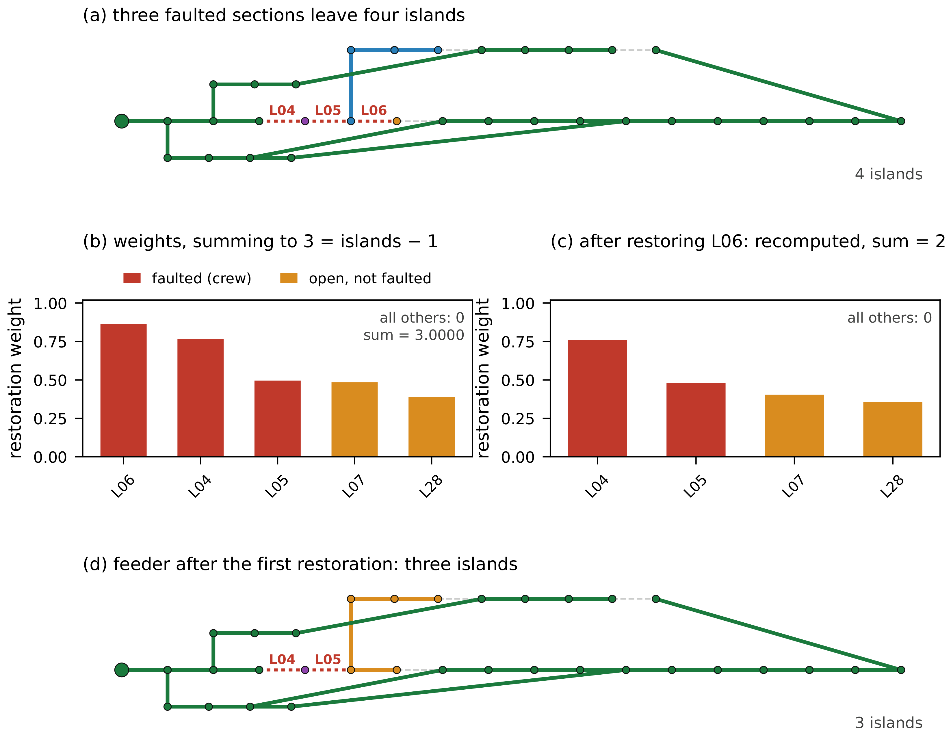
Sections L04, L05 and L06 are lost, leaving four islands. Algorithm 1 gives the weights of

Table 5. The worked outage of Section 4.7: restoration weights, summing to 3.0000, beside the load each restoration would reconnect. All sections not listed have weight zero.

Section	Nodes	Kind	Weight	Capacity Reconnected
L06	6–7	faulted	0.8644	0.000
L04	4–5	faulted	0.7654	0.032
L05	5–6	faulted	0.4958	0.000
L07	7–8	open, not faulted	0.4845	0.038
L28	28–29	open, not faulted	0.3899	0.123

, summing to $3.0000$ as Corollary 1 requires. Note that L07 and L28 are ordinary built-out sections that happen to stand open in the configuration the faults struck; they are not tie sections. Figure 4 shows the islands and the weights before and after the first restoration.

The list is read as a structural diagnostic, and three features of it are worth naming. The zero weights are actionable and exact: every section outside the five listed has weight zero, meaning its terminals are already joined through energised sections, so restoring it would close a loop and cannot reduce the island count at this step. The weights say how replaceable each restoration is: weight $0.8644$ on L06 means a large share of the admissible completions pass through it, and a weight approaching one would mean it is the only remaining connection between two islands; in this scenario no candidate is unavoidable, which is itself information. The weights do not point at the substation: the section with the largest weight reconnects no load at all, while the largest load is reconnected by L28 with weight $0.3899$. The kernel is built from a symmetric network and contains no distinguished node, so it cannot and does not rank restorations by load recovered.

4.8. The Weights Are Not a Dispatch Order

Because (5) is canonical it is tempting to read it as a repair priority. We tested that reading and it fails, and we report the failure because the temptation is strong and the consequence of yielding to it is a worse restoration sequence.

Over 250 episodes, with faults drawn uniformly from a configuration of the operating ensemble and nodal demands as in Appendix A, we compared four policies: ordering by the weights; greedy service, restoring the section that reconnects the most load; working outward from the substation; and random order. The metric is the fraction of feeder load connected to the substation after j restorations.

Table 6. Served capacity after j restorations, three faulted sections, 250 episodes: mean over the episodes, with the standard error of the mean in parentheses. All four policies are evaluated on the same episodes.

Policy	$\mathit{j}=0$	$\mathit{j}=1$	$\mathit{j}=2$	$\mathit{j}=3$
weights (5)	0.4306 (0.0178)	0.5505 (0.0156)	0.6767 (0.0153)	1.0000
greedy service	0.4306 (0.0178)	0.8030 (0.0087)	0.9451 (0.0027)	1.0000
outward from the bus	0.4306 (0.0178)	0.6838 (0.0134)	0.8706 (0.0086)	1.0000
random order	0.4306 (0.0178)	0.5736 (0.0195)	0.7416 (0.0187)	1.0000

reports the mean over the episodes with the standard error of the mean; the four policies are run on the same 250 episodes, so the differences between rows are paired. The dispersion across episodes is large, of the order of $0.25$, because the episodes differ in how much load the three faults cut off.

Ordering by the weights recovers load more slowly than greedy service and more slowly than working outward from the substation, by margins of many standard errors, and no faster than random order: the paired difference between random order and the weights is $+0.023\pm 0.019$ after one restoration and $+0.065\pm 0.021$ after two, so the weights are indistinguishable from random order at the first step and behind it thereafter. The reason is structural and visible in the definition: the kernel is built from a symmetric network with no distinguished node, so the weights know nothing about where the substation is, and a mechanism blind to the source cannot prioritise service to it.

Nor do the weights maximise the feeder’s remaining freedom. Writing $Z\left(H\right)$ for the weighted number of spanning trees of H, the weight admits the third form

$$\frac{\det Y_{B\cup e}}{\det Y_B}=g_e\frac{Z(G/(B\cup e\left)\right)}{Z(G/B)},$$

(6)

verified numerically to $1.2\times {10}^{-15}$, so the weight is the share of admissible completions passing through e, a share carrying the factor $g_e$ and therefore pulled towards low-resistance sections. In our episodes random order retains marginally more freedom than the weights do.

What the comparison establishes is a division of roles. For deciding where to send a crew, use a service-based ordering; nothing in this paper improves on greedy service for that purpose. For the model, the mechanism (5) is a canonical representative rather than a necessity. By Proposition 3 the determinantal form and the per-section statements of Section 5 hold for any repair that intertwines the sectors at the same total rate, and other conductance-aware intertwiners exist, as Remark 3 shows. What (5) alone does is reverse the fault, which makes it the unique member of that class with a reversible stationary law. By Proposition 4 the occupancy indices survive even repair policies that do not intertwine the sectors, provided the total rate is the same. For diagnosis, the weights carry information no service ordering contains which restorations are unavoidable, which are redundant at the current step, and how much of the completion mass each candidate carries.

Section 6 exhibits a milder case. In the generator layer the same determinant ratio measures novelty of a unit’s output profile relative to what is running, which is at least a quantity an operator might care about, whereas here it measures nothing the utility wants. Even there the alignment is empirical rather than proved. Whether a canonical mechanism is also a useful rule is never settled by the algebra alone.

5. Availability and Reliability in Closed Form

5.1. The Maintained Feeder

Section 4 treated a single fault event. A feeder in service is subject to a stream of them. We model this as a continuous-time Markov process on $\mathcal{I}={\bigcup }_k{\mathcal{I}}_k$. Fix a fault intensity $\gamma >0$ per energised section and a restoration intensity $\beta \ge 0$, and let the generator act on functions of $B\in {\mathcal{I}}_k$ by

$$\left(\mathcal{L}f\right)\left(B\right)=\gamma \sum _{e\in B}\left[f(B\setminus e)-f\left(B\right)\right]+\beta \sum _{e\notin B}\frac{\det Y_{B\cup e}}{\det Y_B}\left[f(B\cup e)-f\left(B\right)\right].$$

(7)

By Lemma 1 the total restoration rate out of a k-section configuration is $\beta (r-k)=\beta \left[\right(\mathrm{islands})-1]$, independent of which sections have failed: the crew effort deployed is proportional to the number of islands to be reconnected. We return in Proposition 5 to a fixed crew.

The state of the process is the set of energised sections. A de-energised section may be faulted and awaiting repair, or healthy and open by switching; the two are different actions on different time scales, and the process does not distinguish them. What is modelled is energised-section occupancy, not component availability: $\gamma$ is the rate at which an energised section ceases to carry load, and $\beta$ the rate at which a de-energised one is brought back, whether by a repair or by a switching operation.

Faults strike energised sections at a common rate $\gamma$. In a real feeder the rate depends on section length, construction, age, condition and exposure, and the assumption is not a notational simplification: uniformity is what makes de-energisation exchangeable, and with section-specific rates ${\gamma }_e$ the sector family is no longer mapped onto itself, so neither Theorem 2 nor the closure of Theorem 5 survives, and the occupancy chain ceases to be autonomous. A weighted analogue would require a deletion mechanism whose rates are matched to the ensemble, and we do not have one; Section 10 returns to this.

5.2. Exact Solvability

Theorem 5

(closure and explicit law). Let ${\nu }_t$ be the law of the process generated by (7) and ${\nu }_0={\sum }_k{w}_k\left(0\right){\mu }_k$ any mixture of sectors. Then ${\nu }_t={\sum }_k{w}_k\left(t\right){\mu }_k$ for all $t\ge 0$, where

$${\dot{w}}_k=\gamma (k+1)w_{k+1}+\beta (r-k+1)w_{k-1}-\left[\gamma k+\beta (r-k)\right]w_k,$$

(8)

the equations of r independent two-state units. If $w\left(0\right)$ is binomial with parameter $p_0$ then $w\left(t\right)$ is binomial with

$$p\left(t\right)=\lambda +(p_0-\lambda )e^{-(\beta +\gamma )t},\lambda =\frac{\beta }{\beta +\gamma },$$

(9)

and ${\nu }_t=\mathrm{DPP}\left(p\left(t\right)Y\right)$ for all $t\ge 0$. The stationary law is $\mathrm{DPP}\left(\lambda Y\right)$ and the occupancy relaxes at rate $\beta +\gamma$.

Proof. 

The death part applied to ${\mu }_k$ has exit rate $\gamma k$ and post-jump law ${\mu }_{k-1}$ by Theorem 2; the birth part has the configuration-independent exit rate $\beta (r-k)$ by Lemma 1 and post-jump law ${\mu }_{k+1}$ by Theorem 4. Hence the span of the sectors is invariant and the coefficients obey (8), whose rates are those of r independent binary units, so a binomial initial condition propagates as binomial with $\dot{p}=\beta (1-p)-\gamma p$. It remains to identify the binomial mixture as a determinantal law, which is Proposition A1 of Appendix B.    □

The case $p_0=1$ is the one an engineer starts from: a fully commissioned, radially complete feeder.

The proof used two properties of the upward mechanism and no others: that the total rate out of a configuration in sector k is $\beta (r-k)$, the same for every configuration in that sector, and that the post-jump law is ${\mu }_{k}U={\mu }_{k+1}$. Neither is peculiar to the determinant-ratio kernel, and it is worth recording what that implies.

Proposition 3

(the closure does not need the canonical repair). For each $k<r$ let $U_k$ be any Markov kernel from ${\mathcal{I}}_k$ to ${\mathcal{I}}_{k+1}$, supported on single-section additions, with ${\mu }_k{U}_k={\mu }_{k+1}$, and let the upward rates be $q(B,C)=\beta (r-k)U_k(B,C)$ for $B\in {\mathcal{I}}_k$. Then every statement of Theorem 5 remains valid verbatim, including ${\nu }_t=\mathrm{DPP}\left(p\left(t\right)Y\right)$ and the stationarity of $\mathrm{DPP}\left(\lambda Y\right)$.

Proof. 

Immediate from the proof of Theorem 5, which uses only the two properties just named.    □

The determinant-ratio kernel is therefore not distinguished by making the dynamics exactly solvable; the whole class of sector intertwiners does that. It is distinguished by Proposition 2, as the unique time reversal of uniform deletion, and consequently as the unique member of the class for which the stationary law is reversible in the sense of Corollary 4. On the triangle of Remark 3, with $\beta =3$ and $\gamma =1$, every member $U_a$ of the one-parameter family reproduces $\mathrm{DPP}\left(p\right(t\left)Y\right)$ to $2\times {10}^{-14}$ in total variation and leaves $\mathrm{DPP}\left(\lambda Y\right)$ stationary to ${10}^{-16}$, while the detailed-balance residual is $0.188$ at $a=0$, $0.094$ at $a=1/4$ and exactly zero only at $a=1/2$, the determinant-ratio rule.

5.3. Structural Availability Measures

Corollary 2.

Under $\mathrm{DPP}\left(pY\right)$ with $p=p\left(t\right)$:

(i) 

The number of energised sections is $\mathrm{Bin}(r,p)$;

(ii) 

The number of islands is $1+\mathrm{Bin}(r,1-p)$, with stationary mean $1+(N-1)\gamma /(\beta +\gamma )$;

(iii) 

The feeder is radially complete with probability $p^{N-1}$;

(iv) 

Section e is energised with probability $p{Y}_{ee}$;

(v) 

The joint law of any k switching states is $\det {\left(pY\right)}_S$.

Item (ii) is the simplest of these measures: the expected number of islands is one plus the number of switchable sections times the fault duty cycle $\gamma /(\beta +\gamma )$, and it involves no topology beyond N. Topology enters (iii) and (iv).

These are structural availability measures. They are not the customer-based indices utilities report—SAIFI, SAIDI, CAIDI, EENS—which depend on which sections are de-energised and on how many customers sit behind them. The exact sampler of Corollary 3 supplies the configurations needed to evaluate those by simulation; deriving them in closed form from the kernel is left for future work.

Proposition 4

(the occupancy indices do not depend on the repair policy). Replace the repair mechanism by any allocation of the same total rate $\beta (r-k)$ among the admissible candidates, in particular by service priority, which places the whole rate on the candidate reconnecting the most load. Then the number of energised sections evolves exactly as before, so (i), (ii) and (iii) of Corollary 2 continue to hold. Statements (iv) and (v) need not hold; by Proposition 3 they do hold whenever the allocation intertwines the sectors, and service priority is not such an allocation.

Proof. 

Out of any configuration in sector k the total exit rates are $\gamma k$ downwards and $\beta (r-k)$ upwards, whatever the allocation. The occupancy is therefore an autonomous Markov chain with the rates of (8), and (i)–(iii) are functions of it alone.    □

We verified this on a network small enough to enumerate its 194 admissible partial configurations and compute the stationary law of both mechanisms exactly. Under service-priority repair the stationary law lies at total-variation distance $0.351$ from $\mathrm{DPP}\left(\lambda Y\right)$, with per-section probabilities departing from $\lambda Y_{ee}$ by as much as $0.211$; yet the occupancy law reproduces the binomial to ${10}^{-16}$, the expected island count is $2.000000$ against the formula $1+r(1-\lambda )=2$, and the probability of radial completeness is $0.327680$ against ${\lambda }^r=0.327680$. Service-priority repair also delivers the higher served load, $3.95$ against $3.34$, consistent with Section 4.8.

The division is sharp. The occupancy measures of Corollary 2(i)–(iii) are robust to how the crew is dispatched; the determinantal form and the per-section profile are not.

Corollary 3

(exact sampling). A sample of $\mathrm{DPP}\left(pY\right)$ is obtained by drawing an admissible configuration from the operating ensemble and de-energising each of its sections independently with probability $1-p$. The model class is closed under independent thinning, and quantities not available in closed form, such as the number of served nodes, are obtained by cheap exact sampling.

5.4. Reversibility, and What the Determinantal Form Costs

Corollary 4

(detailed balance). Let ${\pi }_{\lambda }\left(B\right)={\lambda }^{\left|B\right|}{(1-\lambda )}^{r-\left|B\right|}\det Y_B$, the mass function of $\mathrm{DPP}\left(\lambda Y\right)$. Then ${\pi }_{\lambda }\left(B\right)\beta \det Y_C/\det Y_B={\pi }_{\lambda }\left(C\right)\gamma$ for $C=B\cup \left\{e\right\}$, which reduces to $\beta (1-\lambda )=\gamma \lambda$. The process is reversible with respect to $\mathrm{DPP}\left(\lambda Y\right)$.

Proposition 5

(fixed crew). Replace the birth part of (7) by a total restoration rate β independent of the configuration, allocated in proportion to the weights. Then the sector closure still holds, but the occupancy chain has birth rates β and death rates $\gamma k$, with stationary law the truncated Poisson $w_k\propto {(\beta /\gamma )}^k/k!$ on $\{0,\dots ,r\}$. The stationary configuration law is the corresponding mixture of sectors, which is not determinantal.

The contrast is informative rather than a defect. Determinantal form at all times is bought by the assumption that repair capacity follows damage; if capacity is capped, the feeder still stays within the sector family, so the restoration weights, the ladder identity and the exactness of blind faults all survive, but occupancy concentrates differently. Both cases are one-dimensional and solvable; only the first is determinantal.

Corollary 5

(seasonal and campaign maintenance). Let $\beta \left(t\right)\ge 0$ and $\gamma \left(t\right)>0$ be piecewise continuous. Then the closure remains valid with (9) replaced by the solution of $\dot{p}=\beta \left(t\right)(1-p)-\gamma \left(t\right)p$. A feeder started from $\mathrm{DPP}\left(p_{0}Y\right)$ and maintained under any schedule is a determinantal feeder with kernel $p\left(t\right)Y$ at every instant. No stationary law and no uniform relaxation rate are claimed in this case.

Planning availability thus reduces to a one-dimensional deterministic control problem for $p\left(t\right)$, around which the realised number of energised sections fluctuates with binomial statistics.

5.5. Numerical Illustration and Scope

Table 7. Structural availability measures under independent thinning: Monte Carlo estimates from 60,000 independent draws of the exact sampler of Corollary 3, with the standard error of each estimate in parentheses, against the closed forms of Corollary 2.

p	Energ. (MC)	Energ. (Exact)	Islands (MC)	Islands (Exact)	Nodes Served (MC)	$\mathrm{Pr}\left[\mathbf{Complete}\right]$ (MC)	(Exact)
0.99	31.68 (0.002)	31.68	1.32 (0.002)	1.32	30.33 (0.03)	0.727 (0.002)	0.725
0.97	31.04 (0.004)	31.04	1.96 (0.004)	1.96	25.73 (0.04)	0.377 (0.002)	0.377
0.95	30.40 (0.005)	30.40	2.60 (0.005)	2.60	21.93 (0.04)	0.193 (0.002)	0.194
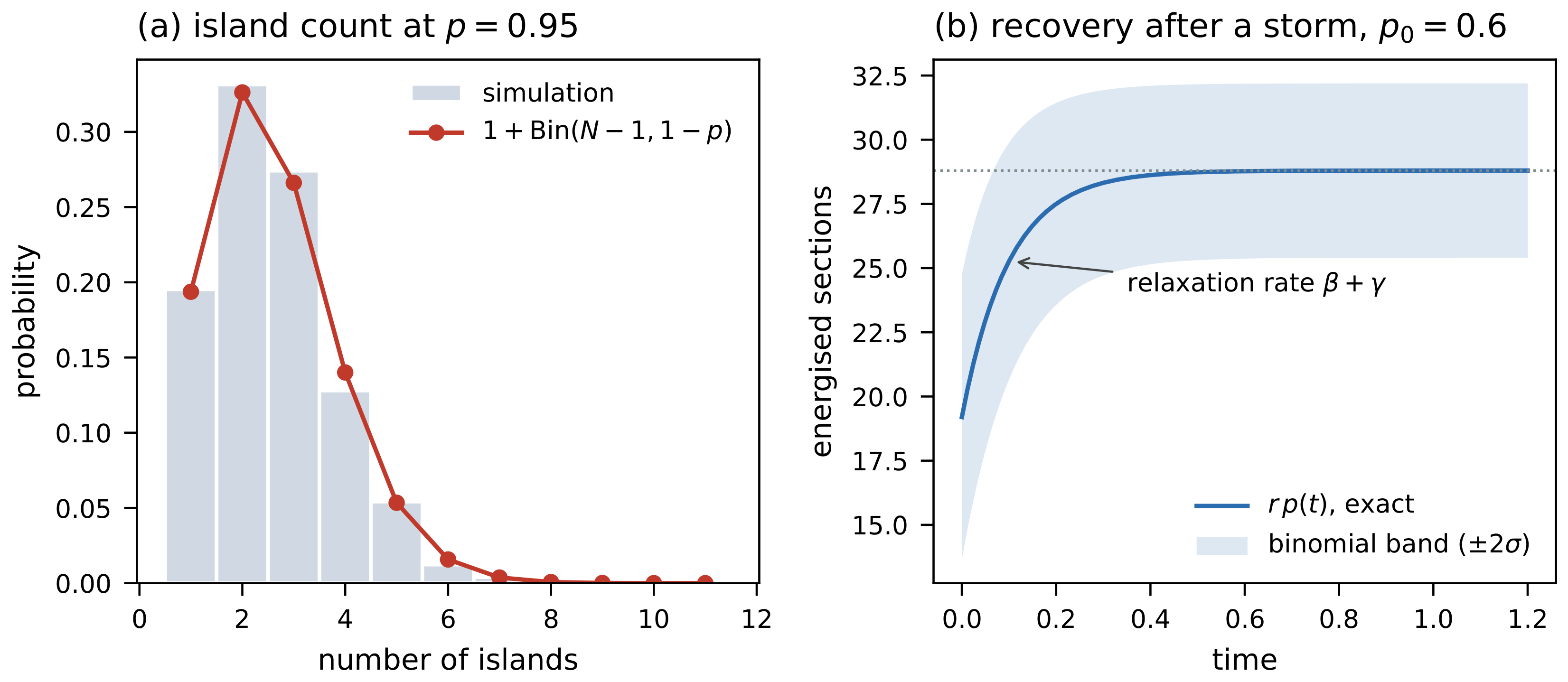
0.90	28.80 (0.007)	28.80	4.20 (0.007)	4.20	15.31 (0.04)	0.035 (0.001)	0.034

sets the closed forms of Corollary 2 beside Monte Carlo estimates at four values of the per-section availability.

The Monte Carlo columns rest on 60,000 independent draws of the exact sampler, and their standard errors are reported in the table; the exact columns carry none. The section and island counts are reproduced by the formulas to sampling accuracy; the served-node column uses the exact sampler of Corollary 3, since it depends on which sections are energised and not only on how many. At a per-section availability of $0.95$ the feeder is fully connected less than one-fifth of the time, while the expected number of islands is still under three. Figure 5 shows the island-count distribution at that availability and the recovery of the section count after a storm.

Theorem 5 rests on two assumptions. Repair intertwines the sectors at total rate $\beta (r-k)$: by Proposition 3 any such repair, canonical or not, gives the determinantal form and (iv) and (v) of Corollary 2, while (i)–(iii) need only the total rate, by Proposition 4. Faults strike energised sections independently and uniformly: this is the appropriate model for the accumulation of unrelated defects and not for a single event damaging several adjacent sections, and Section 10 quantifies the departure and sets out the three levels at which the results of this paper assert anything about a real feeder.

6. Distributed Generators: The Same Calculus on a Different Ground Set

6.1. A Second Failure Layer

A feeder carrying distributed generation fails in a second, independent way: the generators themselves drop out through converter trips, protection operations, mechanical faults or maintenance, while the network remains intact. The ground set is now the n generators, and substitutability is not topological: two units are substitutes when their output profiles are alike. The entire calculus transfers without modification, because the algebraic proof of Lemma 1 used only that Y is an orthogonal projection.

6.2. The Generation-Mode Projection, and What It Is Not

Let X be the $T\times n$ matrix of measured output, each column divided by the installed capacity of its unit. Centre X, compute its singular value decomposition, retain the r leading right singular vectors as the rows of an $r\times n$ matrix $\mathsf{\Psi }$ with orthonormal rows, and set

$$P={\mathsf{\Psi }}^{\top }\mathsf{\Psi },P=P^{\top }=P^2,\mathrm{rank}P=r.$$

(10)

The rows of $\mathsf{\Psi }$ are the generation modes; the jth column is the loading vector of unit j; and $\det P_B$ is the squared r-dimensional volume spanned by the loadings in B, as in volume sampling [37,38].

Two properties of this geometry must be stated at once, because they bound what the calculus may claim. First, the construction is whitened: $\mathsf{\Psi }$ has orthonormal rows, so the singular values of the output matrix have been divided out. The physical profile of unit j restricted to the retained subspace is ${\mathsf{\Sigma }}_r{\psi }_j$ and not ${\psi }_j$, so a determinant ratio built from P is not a marginal gain in output variance. Second, in the whitened geometry the natural coverage functional is degenerate: writing ${\mathsf{\Pi }}_B$ for the orthogonal projection onto the span of the loading vectors indexed by B, one has $\parallel {\mathsf{\Pi }}_B{\mathsf{\Psi }\parallel }_F^2/\parallel \mathsf{\Psi }{\parallel }_F^2=\mathrm{tr}\left({\mathsf{\Pi }}_B\mathsf{\Psi }{\mathsf{\Psi }}^{\top }\right)/r=k/r$ for every independent B, because $\mathsf{\Psi }{\mathsf{\Psi }}^{\top }=I_r$. Whichever k units are running, the whitened coverage is the same number. We therefore call the quantity below a geometric novelty score, not a coverage gain, and we claim no output-variance optimality for it anywhere.

The rank r is the number of independent generation regimes the fleet can distinguish. The sector laws are ${\mu }_k\left(B\right)={\left(\genfrac{}{}{0pt}{}{r}{k}\right)}^{-1}\det P_B$.

Proposition 6.

Lemma 1 holds verbatim for P, and $S_{jj}=\det P_{B\cup j}/\det P_B$ equals the squared norm of the component of the loading vector of unit j orthogonal to the span of the loading vectors of the units in B.

Proof. 

The first statement is the algebraic proof of Lemma 1, which used only $P^2=P$ and $\mathrm{tr}P=r$. For the second, $S_{jj}$ is the Schur complement $P_{jj}-P_{jB}{P}_{BB}^{-1}{P}_{Bj}$, and $P_{BB}$ is the Gram matrix of the loading vectors indexed by B.    □

So $S_{jj}$ is the squared residual novelty of unit j in the whitened retained-mode geometry—the part of its loading vector ${\psi }_j$, not of its physical profile ${\mathsf{\Sigma }}_r{\psi }_j$, that the running units do not span. Summed over the failed units these residuals give $r-\mathrm{rank}{\mathsf{\Psi }}_B$, the number of generation regimes not currently covered; when the running loadings are linearly independent this is $r-\left|B\right|$.

6.3. Blind Loss, Blind Repair, and the Repair Rule

Theorem 6.

Let generators fail independently and uniformly at random. Then the surviving fleet is distributed exactly as the sector law of the corresponding size, for any number of failures; and no repair rule chosen independently of P can return the fleet to the sector family for all rank-r projections P with $r<n$. The rule $U(B,B\cup j)=\det P_{B\cup j}/\left((r-k)\det P_B\right)$ is stochastic and satisfies ${\mu }_{k}U={\mu }_{k+1}$; upward intertwiners are not unique, by Remark 3, and what singles this one out is that it is the unique kernel reversing uniform blind loss.

Remark 4.

The witnesses in the impossibility argument (Appendix B) are degenerate fleets. The obstruction is not an artefact of that degeneracy: the set of projections for which a given candidate rule fails is open, so failure persists on a neighbourhood of each witness.

Two distinct objects share this score and should not be conflated. Theorem 6 describes a stochastic kernel: it restores unit j with probability proportional to $S_{jj}$, and it is that randomised mechanism which reverses blind loss and carries one sector onto the next. Algorithm 2 restores instead the maximiser of $S_{jj}$. Greedy selection reverses nothing, does not map the sector family onto itself, and inherits none of the exactness statements of this section; it is a heuristic suggested by the same geometry, and we present it as one.

The parallel with the network layer is exact. There, the repair weight is the resistance seen across a section once everything still energised has been shorted; here, it is the residual of an output profile once everything still running has been projected out. In both cases the weights sum to the number of gaps: islands minus one there, uncovered modes here.

Algorithm 2 Fleet repair by novelty score

Offline, once: from the output history compute $\mathsf{\Psi }$ and P. 1: Let B be the units currently running and F the failed units. 2: Form ${\mathsf{\Psi }}_B$ and compute a QR factorisation of ${\mathsf{\Psi }}_B^{\top }$. 3: For each $j\in F$ compute $S_{jj}={\parallel (I-Q{Q}^{\top }){\mathsf{\Psi }}_{:,j}\parallel }^2$. 4: Check ${\sum }_{j\in F}{S}_{jj}=r-\mathrm{rank}{\mathsf{\Psi }}_B$, which the QR of step 2 supplies; abort on mismatch. When the running loadings are independent this reads $r-\left|B\right|$, but the rank form is the one to implement, since a running fleet may well contain redundant units. 5: Dispatch to $\arg {\max }_j{S}_{jj}$; on repair move j to B and return to step 2.

6.4. Worked Example: The Model Fleet

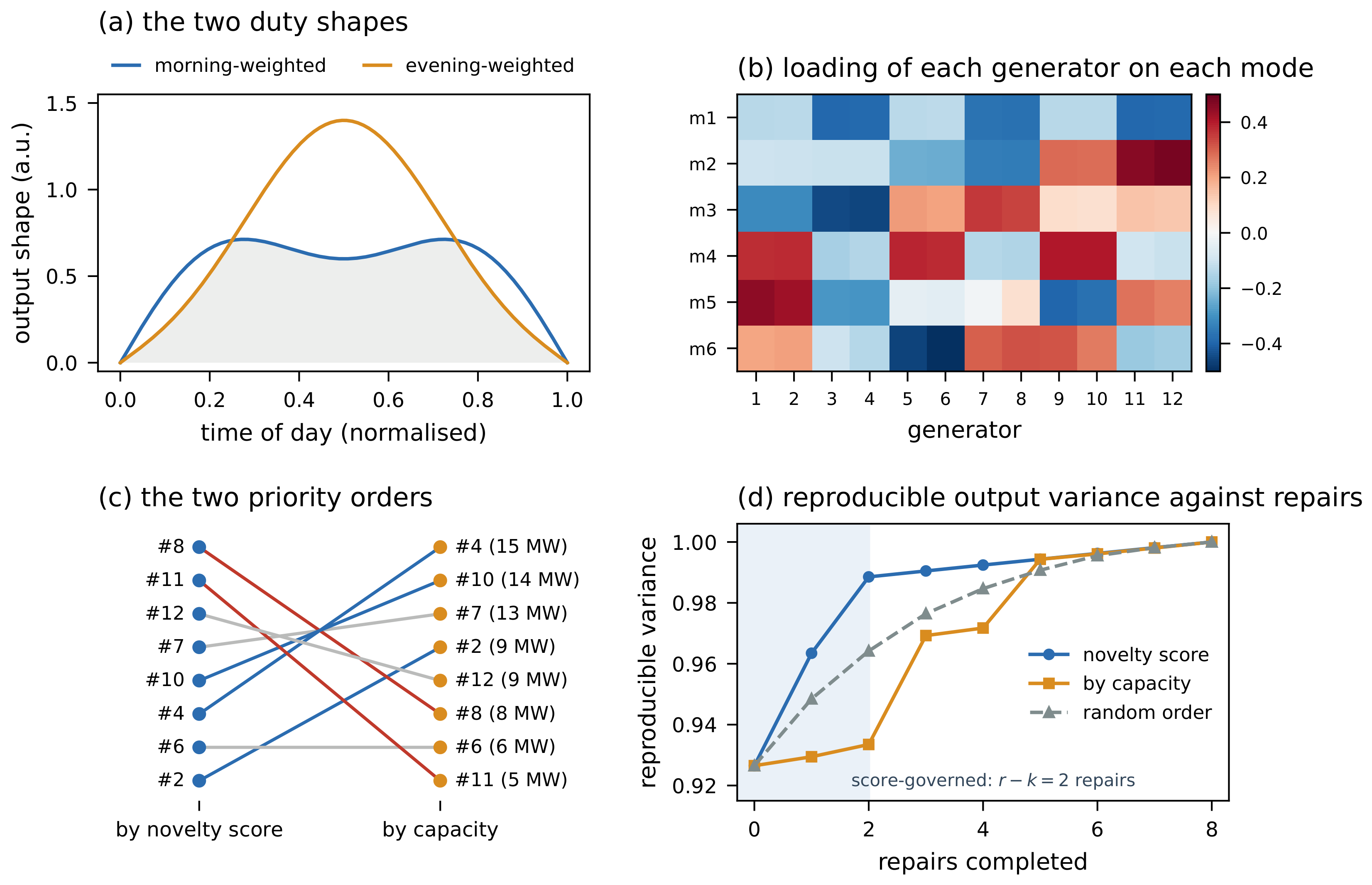
The model fleet has twelve units in three clusters, each with two morning-weighted and two evening-weighted profiles, $r=6$ generation modes and capacities between 5 and 15 MW; four units are running and eight are down.

Table 8. Restoration priority for the generator fleet by novelty score (left) and by installed capacity (right); the scores sum to 2.0000, the number of uncovered generation modes; # denotes the unit number.

Rank	Unit	Weight	MW	Unit	MW	Its Weight
1	#8	0.5095	8	#4	15	0.0007
2	#11	0.5005	5	#10	14	0.0010
3	#12	0.4986	9	#7	13	0.4890
4	#7	0.4890	13	#2	9	0.0002
5	#10	0.0010	14	#12	9	0.4986
6	#4	0.0007	15	#8	8	0.5095
7	#6	0.0004	6	#6	6	0.0004
8	#2	0.0002	9	#11	5	0.5005

ranks the failed units by novelty score and, beside it, by installed capacity.

The two orders are almost reversed at the top, and the reason is structural. Unit #4 is the largest at 15 MW and carries the lowest score: it shares a cluster and a duty profile with unit #3, which is running, so its profile is already reproduced and restoring it adds capacity but no new regime. Unit #8, at 8 MW, covers a regime nothing running covers.

The normalised determinantal restoration kernel applies only below the rank, since its factor ${(r-k)}^{-1}$ is undefined at $k=r$; on this fleet that leaves the first $r-k=2$ repairs. The geometric score $S_{jj}$ itself remains defined throughout and simply vanishes once the running units span the retained mode space, which is what happens here after two repairs. Beyond the rank, by Proposition 7, blind addition is exact and the projection-geometric criterion ceases to distinguish candidates at all. It does not follow that no ordering can beat any other: capacity, energy, location and any regime outside the retained rank continue to distinguish them, and only this criterion falls silent. The curves show the criterion falling silent: they separate sharply over the two score-governed repairs and then converge. After those two repairs the variance not reproducible from the running units is $5.8$ times larger under capacity ranking and $3.2$ times larger under random order. The trade-off is explicit: over the same two repairs the score recovers 13 MW against 29 MW for the capacity policy.

The metric plotted in Figure 6d is the physical one, and we define it explicitly because it is not the quantity the score optimises. Writing X for the centred, capacity-normalised output matrix and $X_B$ for its columns indexed by the running units, the reproducible output variance is

$$\mathcal{R}\left(B\right)=\frac{{∥{\mathsf{\Pi }}_{\mathrm{col}\left(X_B\right)}X∥}_F^2}{{\parallel X\parallel }_F^2},$$

(11)

the fraction of the fleet’s output variance recoverable by least squares from the units that are running. Unlike the whitened coverage of Section 6, this quantity does depend on which units are running, because it carries the singular values that the whitening divides out.

6.5. Which Objective This Serves, and Above the Rank

We state the boundary plainly, because the temptation here is the mirror image of the one resisted in Section 4.8. There the determinant ratio optimises nothing the utility wants; here it optimises something geometric, and the question is whether that something is what an operator wants. It is not the same thing as output variance, for the reason given above, and the two orderings genuinely differ: on the model fleet the novelty score ranks unit 8 first while the marginal gain in $\mathcal{R}$ of (11) ranks unit 12 first, though the leading four units are the same set and their variance gains are within four per cent of one another. What can be said is that the score and the physical gain are aligned in this example, not that one optimises the other.

If the objective is recovered energy, the correct dispatch is by lost capacity and no calculus is needed. The score measures novelty of a unit’s profile relative to what is running, which matters when the feeder carries a firm-capacity or ramp obligation, when forecast quality is contractually relevant, or when the exposure of concern is correlated shortfall rather than annual yield. In practice a planner often wants both, and the natural compromise is to rank by the product of installed capacity and novelty score; we note explicitly that this hybrid is a heuristic to which none of the exactness statements apply.

Proposition 7

(the mirror). For $r\le s\le n$ let the fleet law above the rank be

$${\nu }_s\left(S\right)={\left(\genfrac{}{}{0pt}{}{n-r}{s-r}\right)}^{-1}\sum _{B\subseteq S,\left|B\right|=r}\det P_B\propto \det \left({\mathsf{\Psi }}_S{\mathsf{\Psi }}_S^{\top }\right),\left|S\right|=s,$$

the two forms agreeing by Cauchy–Binet, where ${\mathsf{\Psi }}_S$ is the $r\times s$ submatrix of loading vectors indexed by S; this is the squared r-dimensional volume of the frame carried by S, which is the right generalisation once $s>r$ makes an s-dimensional volume meaningless. Then S has the law of a core $B\sim {\mu }_r$ together with a padding of $s-r$ units chosen uniformly among the rest; blind addition maps the law of size s onto that of size $s+1$ exactly, and blind removal does not.

In an over-provisioned fleet the geometric criterion is silent on restoration order, while the decisions it does speak to are the ones that take units out of service: planned outages, curtailment allocation and maintenance scheduling should be made with the residuals in hand. Theorem 5 applies verbatim with Y replaced by P, so the fleet has the determinantal law with kernel $p\left(t\right)P$ at every instant and the expected number of covered modes is $rp\left(t\right)$.

The construction needs an output history long enough to estimate r modes stably, in practice one to two years of sub-hourly data, together with a reliable capacity normalisation. Three cautions apply: the modes must be estimated on outage-free periods, or the outages will be fitted as modes; ageing and seasonal drift move the loadings slowly, so P should be re-estimated on a rolling window; and the failure model is independent failure, which excludes exactly the events that strike neighbouring units together.

7. Reinforcing the Feeder: How the Ensemble Moves

7.1. Transport of the Kernel

Conductors are replaced and existing sections reinforced. These are multi-year decisions and they change g, hence Y and hence every index above. Theorem 7 assumes a fixed edge set and a smooth positive path of conductances, so it covers reconductoring and reweighting but not the installation of a new tie, which sends a conductance from zero and is a jump rather than a drift; Section 8 treats that case.

Theorem 7

(transport of the kernel). Let $g\left(t\right)$ be any smooth positive path of conductances and $Y\left(t\right)$ the kernel (2). Put $\Delta \left(t\right)=\frac{1}{2}\mathrm{diag}\left(\mathrm{d}\log g_e/\mathrm{d}t\right)$. Then

$$\dot{Y}=(I-Y)\Delta Y+Y\Delta (I-Y),$$

(12)

and consequently $\mathrm{tr}\dot{Y}=0$: the total participation ${\sum }_e{Y}_{ee}$ stays equal to $N-1$. On the diagonal,

$${\dot{Y}}_{ee}=\sum _f\frac{\mathrm{d}\log g_f}{\mathrm{d}t}\left({\delta }_{ef}{Y}_{ff}-Y_{ef}^2\right).$$

(13)

Proof. 

Let $M=G^{1/2}B$, so $\dot{M}=\Delta M$ and $Y=M{M}^{+}$ is the orthogonal projection onto $\mathrm{ran}M$, with $YM=M$. Differentiating, $\dot{Y}M=(I-Y)\Delta M$, hence $\dot{Y}Y=(I-Y)\Delta Y$. From $Y^2=Y$, $\dot{Y}=\dot{Y}Y+Y\dot{Y}$, and the second term is the transpose of the first, namely $Y\Delta (I-Y)$. Adding gives (12); the trace of each summand vanishes because $\mathrm{tr}[\Delta Y(I-Y\left)\right]=0$. Expanding on the diagonal gives (13).    □

Equation (12) is the classical derivative of an orthogonal projection onto a moving subspace [39], and we claim no novelty for the identity itself. What is used here is its instantiation: the driver $\Delta$ is exactly one half the logarithmic rate of change in the conductances, so a reinforcement schedule is fed directly into (12) and the resulting motion of every index is read off. Here $\Delta$ is immediate, with no eigenvector to differentiate, because the conductances are the primitive quantities.

7.2. Exact Planning Sensitivity

Corollary 6.

Reinforcing a single section e, at fixed conductances elsewhere,

$$\frac{\partial Y_{ff}}{\partial \log g_e}=-Y_{ef}^2(f\ne e),\frac{\partial Y_{ee}}{\partial \log g_e}=Y_{ee}(1-Y_{ee}),$$

and the sum of these changes over all sections is exactly zero.

Three consequences are worth stating in the operator’s language. Reinforcement redistributes redundancy, it does not create it: the total participation is pinned at $N-1$ by Foster’s rule, so every point a section gains is lost by others, allocated by the squares of the couplings, which is precisely the substitution map of Proposition 1(iii). The price of a reinforcement is computable before it is made. Leverage is highest where certainty is lowest: the self-term $Y_{ee}(1-Y_{ee})$ is a vacancy factor, vanishing for a section energised in every admissible configuration and maximal at $Y_{ee}=1/2$, so investment leverage is concentrated on the sections the feeder is least sure about, which by Table 3 are the tie sections. Finite reinforcements are obtained by integrating, not by extrapolating.

On the benchmark feeder, reinforcing tie T1 by one unit of log-conductance gives itself $+0.2479$ and takes $-0.0489$ from T3, $-0.0410$ from L19, $-0.0251$ from L08, $-0.0195$ from L07 and $-0.0173$ from L21, with total change $4.8\times {10}^{-16}$. Figure 7 shows the full map and the vacancy factor of every section.

7.3. Loading-Driven Sizing and the Loss of Redundancy

Conductor sizing is driven by loading. Written as an optimisation with the conductor budget held fixed, this is the classical problem [40,41,42] of minimising the total ohmic loss

$$P\left(w\right)=b^{\top }L{\left(w\right)}^{+}b\mathrm{subject}\mathrm{to}\sum _e{w}_e=1,$$

(14)

where b is the vector of nodal current injections and $w_e$ is proportional to the cross-section of section e. We take the reference loading of Appendix A: every node drawing current in proportion to its demand, all of it supplied from the substation bus, and currents computed in the full meshed network. By the envelope theorem $\partial P/\partial w_e=-q_e^2/w_e^2$ with $q_e$ the current in section e, so the gradient flow of $-P$ on the simplex is precisely a loading-driven reinforcement.

Integrating that flow and feeding the resulting path into (12) gives the following. Loss-optimal sizing reduces the loss from $87.3$ at uniform sizing to $36.98$, by 58 per cent. It also drives three of the thirty-seven sections to zero conductance and pins seventeen of the thirty-two slots at $Y_{ee}=1$, with ${\min }_e{Y}_{ee}$ falling to zero: the feeder keeps two of its five loops and loses most of its switching freedom. The trace is conserved throughout, as Theorem 7 requires; what is destroyed is not the amount of participation but its spread, and in ensemble terms the restoration weights degenerate on the pinned sections.

The collapse is partial rather than total on this feeder: the loss-optimal sizing is not a tree. The dichotomy between tree-like and loop-retaining optima known for adaptive transport networks [41,43,44] is the neighbouring result, and the computation above is an instance of the same phenomenon rather than an application of that dichotomy. Sizing purely by loading is not a neutral policy that happens to save a conductor: it is a policy that spends the feeder’s switching freedom.

7.4. An Entropic Redundancy Term Removes the Boundary Optima

Proposition 8

(interiority). Let w lie in the relative interior of the simplex, let J be continuously differentiable with bounded partial derivatives near the simplex, and put $F_{\eta }\left(w\right)=J\left(w\right)+\eta H\left(w\right)$ with H the Shannon entropy and $\eta >0$. Then every maximiser of $F_{\eta }$ over the simplex lies in the relative interior and satisfies $w_e\propto \exp \left((\partial J/\partial w_e)/\eta \right)$. In particular no single-section sizing is optimal for any $\eta >0$.

Proof. 

Let w lie on the boundary, say $w_e=0$ and $w_f>0$, and move along $w\left(t\right)=w+t({\delta }_e-{\delta }_f)$. The entropy contributes $-\eta [t\log t+(w_f-t)\log (w_f-t)]$ up to terms independent of t, whose derivative tends to $+\infty$ as $t\downarrow 0$, while $\mathrm{d}J/\mathrm{d}t$ stays bounded. Hence $F_{\eta }$ increases and w is not a maximiser. An interior maximiser is a constrained critical point, which is the stated Gibbs form.    □

The redundancy weight $\eta$ is distinct from the availability $\lambda =\beta /(\beta +\gamma )$ of Section 5. The result is specific to the entropic penalty and does not hold for redundancy terms in general: what drives the optimum inward is the infinite inward slope of H at the boundary, and a quadratic diversity penalty, for instance, has no such property. The transition at $\eta =0$ is accordingly abrupt rather than gradual.

The hypothesis on J deserves a word, because for the loss objective (14) it is not satisfied on the whole simplex. By Lemma A3, $\partial (-P)/\partial w_e=\Delta {\phi }_e^2$, the squared potential difference across the section, which is bounded on any region where the support of w remains connected and diverges only as a bridge is driven towards zero conductance. That divergence pushes the bridge’s weight up: the singular boundary at which the support disconnects is repelling for the loss objective rather than attracting. On the connected-support region the mechanism of Proposition 8 therefore applies, and the benchmark computation below confirms interiority; we do not claim a separate proof for $P\left(w\right)$ on the whole simplex. Operationally the rest point is a Gibbs, or logit, allocation in which the utility of a section is its marginal contribution to the objective and $\eta$ is the weight placed on keeping the feeder reconfigurable; a redundancy standard, a minimum-section rule or an explicit diversity term all act as such an $\eta$.

Table 9. Dissipation against retained switching freedom at the rest point of the tempered sizing flow; $\eta$ is the redundancy weight of Proposition 8.

$\mathit{\eta }$	P	Excess	Dead	Pinned	${\min }_{\mathit{e}}{\mathit{Y}}_{\mathit{ee}}$
uniform	87.32	+136%	0	1	0.7492
0	36.98	+0.0%	3	17	0.0000
5	37.11	+0.3%	0	21	0.0113
10	37.62	+1.7%	0	1	0.2694
20	39.41	+6.6%	0	1	0.5796
50	44.47	+20.2%	0	1	0.7441

reports the rest point of the tempered sizing flow on the benchmark feeder for several values of the redundancy weight.

The headline, on the benchmark feeder, is the row at $\eta =10$: an excess of $1.7$ per cent over the loss-optimal sizing buys back the feeder’s switching freedom in full, with no section driven to zero and only the structural bridge pinned. Two qualifications belong with it. The benchmark optimisation is interior for every $\eta >0$ tested, and interiority is already reached near $\eta =5$, but interiority is not the same as usable freedom: there twenty-one slots are still pinned and ${\min }_e{Y}_{ee}=0.011$, so the practically relevant threshold is higher than the mathematical one. And the count of pinned slots is not monotone in $\eta$, so the recovery is sharp rather than gradual and occurs between $\eta =5$ and $\eta =10$ on this feeder (Figure 8). The threshold and the size of the penalty are properties of this network and its loading, not a general planning conclusion.

A candidate reinforcement programme is a path $g\left(t\right)$; integrating (12) along it returns the whole trajectory of the operating ensemble, so candidates can be compared not only by loss reduction, which standard tools already provide, but by what they do to the feeder’s ability to reconfigure. Corollary 6 is exact for the ensemble of admissible topologies and says nothing about voltages, currents or losses at the operating point, which remain the province of load-flow analysis; the two are complementary and should be run together. Equation (14) represents one investment criterion, minimum loss at fixed conductor budget; a planner with a different objective should substitute it into Proposition 8 directly.

8. Two Clocks

8.1. Separation of Time Scales, and What Exactly Lags

Faults and repairs move the occupancy on the time scale of the maintenance cycle, with relaxation rate $\beta +\gamma$: days to weeks. Reconductoring moves the conductances on the time scale of the investment programme: years. The two differ by two to three orders of magnitude, and the question is whether the exact results above may be applied with the current kernel $Y\left(t\right)$.

For a frozen geometry there is no lag of any kind inside a sector: by Theorem 5 the jump mechanisms map the sector family onto itself exactly, so the conditional law given the number of energised sections is ${\mu }_k$ at every instant. This ceases to hold the moment the geometry moves. At time t the law is a mixture of the sectors of $Y\left(t_0\right)$ for whatever earlier $t_0$ it last equilibrated to, and that is not a mixture of the sectors of $Y\left(t\right)$. Re-equilibration of the shape within a shell is a second relaxation process, governed not by $\beta +\gamma$ but by the mixing of the down-up exchange chain on each shell, which is the composition of the two mechanisms of Section 4 and leaves ${\mu }_k$ invariant. Chains of this type mix rapidly [22,23,24], but their rate is a separate quantity. The size of the perturbation is supplied by (12), bounded by $\parallel \Delta \parallel \le \frac{1}{2}{\max }_e|\mathrm{d}\log g_e/\mathrm{d}t|$.

8.2. A Scaling Estimate, Verified Exactly

The statement below is a scaling estimate supported by exact computation, not a theorem: we do not prove it, and we label it accordingly.

Estimate 1

(quasi-static approximation). Let the conductances follow a smooth path $g\left(t\right)$ and let the feeder evolve under (7) built from $Y\left(t\right)$. Put $\epsilon ={\max }_e|\mathrm{d}\log g_e/\mathrm{d}t|/\kappa$, where κ is the spectral gap of the down-up exchange chain on the occupied shells. If the law is initially $\mathrm{DPP}\left(\lambda Y\right(0\left)\right)$, then $\parallel {\nu }_t-\mathrm{DPP}\left(\lambda Y\left(t\right)\right)\parallel =O\left(\epsilon \right)$ uniformly on compact time intervals.

The occupancy rate $\beta +\gamma$ does not appear, because occupancy does not lag. We verified this exactly rather than by simulation. On a network small enough for its 194 admissible partial configurations to be enumerated, we integrated the Kolmogorov equation along a ramp of one conductance and computed the total-variation distance exactly (Figure 9). Three findings. The distance is linear in $\epsilon$: over $\epsilon$ from $0.01$ to $0.08$ the log-log slope is $0.9974$ and $\mathrm{TV}/\epsilon$ is constant at $0.64$; beyond $\epsilon \approx 0.1$ the linear regime ends and the distance saturates. The distance depends on the ramp speed and the process rates only through their ratio: varying either at fixed $\lambda$ produces identical distances at equal $\epsilon$, to every digit computed. And the prefactor is not governed by $\beta +\gamma$: holding $\beta +\gamma$ fixed and varying only the split between them changes $\mathrm{TV}/\epsilon$ by a factor of $7.5$ as $\lambda$ runs from $0.5$ to $0.9$.

We do not track the constant analytically and do not claim exact tracking; this is why the statement is labelled an estimate. A finite-state adiabatic proof would require a uniform lower bound on the shell gaps along the path, which we do not have. What is established is the linear improvement with scale separation, which for the numbers above means a relative error of order ${10}^{-2}$ to ${10}^{-3}$.

8.3. What This Licenses, and Where It Is Not the Right Tool

Freeze the kernel over a planning increment, apply the exact results within it, and recompute when the increment closes. The restoration weights use the kernel as commissioned and need no update between reinforcements; the reliability indices are evaluated at the current Y and are exact within the increment; a reinforcement programme is evaluated by integrating (12) along it. The generator layer has the same structure, with P re-estimated on a rolling window.

Two situations are outside the approximation. A commissioning event is a jump, not a drift: a new tie in particular sends a conductance from zero, where $\log g$ is undefined, so the kernel jumps and the feeder relaxes from a mixture of the old sectors towards the new family, the occupancy part of that transient decaying at rate $\beta +\gamma$ and the shape part not being available in closed form; indices computed immediately after a commissioning carry a transient error of duration of order of the maintenance cycle. A storm, by contrast, is a jump in occupancy and not in geometry and is covered exactly by Corollary 5.

9. Implementation

9.1. Inputs and Cost

For the network layer: the node list; the section list with terminal nodes and resistance, or length, cross-section and conductor material; the switching inventory, and which devices are remotely operable; and the current switching and fault state for online use. For the generator layer: per-unit output at sub-hourly resolution over at least one and preferably two years, installed capacity per unit, and the outage log. Nothing else is required: the restoration weights need no load-flow solution, no weather data, no protection settings and no failure statistics, and $\beta$ and $\gamma$ enter only in the reliability indices.

Offline, once per commissioned topology: assemble $L=B^{\top }GB$; factorise it grounded at the substation bus, at cost $O\left(N^3\right)$ dense and far less with a sparse factorisation, feeders being sparse and close to planar; read off the effective resistances and hence the diagonal of Y; and, if the full kernel is wanted, assemble it from four look-ups per entry at cost $O\left(m^2\right)$. Online, per fault event: a union-find contraction, a factorisation of the reduced Laplacian on $N-\left|B\right|$ nodes, and one effective resistance per candidate. Contraction should be implemented by union-find on node labels, never by matrix surgery on L.

Two identities should be asserted in code. $\mathrm{tr}Y=N-1$ is Foster’s rule, and it is worth being precise about what it validates: the identity holds for every assignment of positive conductances, so it does not detect a mis-entered resistance, but it does detect a duplicated section, a node with no connection, a wrong terminal or an incidence matrix built from a stale asset register. The restoration weights summing to the island count minus one validates the contraction and the bookkeeping of the switching state, which are the parts of the online path most likely to drift out of step with reality.

9.2. Sampling, Attachment and Scale

Indices depending only on how many sections are energised are formulas, by Corollary 2; indices depending on which ones require the configuration and are obtained by exact sampling: draw an admissible configuration by Wilson’s algorithm [17,18] rooted at the substation bus, then de-energise each of its sections independently with probability $1-p$; by Corollary 3 the result is an exact draw from $\mathrm{DPP}\left(pY\right)$. The procedure is exact rather than asymptotic: no burn-in, no convergence diagnostics, no dependence between draws.

Three attachment points, in increasing order of effort. The asset register feeds a kernel service recomputing Y whenever a commissioning changes the topology, whose output is a static per-section table of self transfer-current factor, vacancy factor and strongest substitutes. The outage management system calls Algorithm 1 and returns the restoration weights, which are a structural diagnostic and not a dispatch order, for the reasons of Section 4.8; they should be displayed beside the service-based ordering the utility already uses, which remains the correct basis for deciding where to send a crew. The planning tool integrates (12) along a candidate reinforcement path and reports the configurational cost of each candidate alongside its loss reduction.

The relevant comparison for scale is with enumeration, the only alternative way to obtain the same quantities exactly. Enumeration grows multiplicatively with the number of independent loops and is out of reach at a dozen ties; the cost of the kernel does not grow combinatorially with the number of loops, though it does grow with the size of the network, through m in the storage of the full kernel and N in the factorisation.

The timings of

Table 10. Cost by network size. Configuration counts from the matrix-tree determinant, never by enumeration. Timings are wall-clock, best of repeated runs, in the environment stated in the text.

Feeder	N	m	Configurations	Factorise (ms)	Y Diagonal (ms)	Per Event (ms)
small	33	37	50,751	0.03	0.2	0.23
medium	301	318	${10}^{21.5}$	0.11	3.4	0.33
large	2001	2080	${10}^{113}$	0.80	131	1.18

were obtained on one core of an Intel Xeon processor at 2.10 GHz with 4 GB of memory under Linux, with Python 3.12.3, NumPy 2.4.4, SciPy 1.17.1 and networkx 3.6.1; each entry is wall-clock time, the best of seven repetitions for the factorisation and of three for the other two columns. The scripts are provided as Supplementary Materials.

The full $m\times m$ kernel costs a dense pseudoinverse: $0.02$ s and 1 MB for the medium network, $4.4$ s and 35 MB for the large one. As a check at scale, $\mathrm{tr}Y=2000.0000$ for the large network. Two features of Table 10 are worth naming: the configuration counts come from the matrix-tree determinant, not from enumeration, and are of order ${10}^{113}$ for the large network while being obtained in a millisecond; and the per-event column is the cheapest of the three, because the contracted post-fault network is far smaller than the feeder.

9.3. Using This Alongside Existing Tools

The calculus does not replace the power-flow and reliability tools a utility already runs; it answers questions those tools do not pose.

Table 11. Where the present calculus sits beside the traditional reconfiguration and reliability methods.

	Optimisation-Based Reconfiguration	Analytical Reliability Assessment	This Paper
object	one configuration	one configuration	the whole family of radial configurations
output	the optimum for a stated objective	customer-based indices for that configuration	exact structural statistics over the family
cost	a search, growing with the number of ties	one evaluation per configuration	one Laplacian factorisation
effect of a reinforcement	re-solve	re-evaluate	closed form, $-Y_{ef}^2$ (Corollary 6)
gives a dispatch order	yes	no	no (Section 4.8)
operational feasibility	built into the constraints	assumed	decided by load flow, outside the model (Section 10)

sets it beside the two traditional approaches, and

Table 12. Division of labour between the kernel and the tools a utility already runs.

Question	Answered by
is this configuration operable: voltages, ratings, protection	AC power flow or branch flow
which configuration minimises loss or balances load	existing reconfiguration optimisation
how much switching freedom does the feeder retain, and which devices substitute for which	the kernel Y (Proposition 1)
which restorations are unavoidable, which are redundant at this step	Algorithm 1
where to send the crew	service-based ordering, not this paper (Section 4.8)
how many islands does a maintained feeder carry, how often is it whole	Corollary 2
customer-based indices: SAIFI, SAIDI, CAIDI, EENS	the utility’s reliability tool, fed by the exact sampler of Corollary 3
what a reinforcement costs the configuration space	the transport Equation (12) and Corollary 6

states the division of labour question by question.

The workflow follows from the table. The kernel service runs off the asset register and updates only when a commissioning changes the topology or a resistance; it needs no load data. When a fault occurs, the outage management system calls Algorithm 1 on the current switching state and displays the weights, which are a structural diagnostic, in addition to the service-based ordering it already uses; the crew is sent by the latter. Any configuration the operator intends to close is passed through the alternating-current load flow, which decides voltages, ratings and protection; the kernel cannot and does not do this. For planning, the transport equation is integrated along a candidate reinforcement path in the same tool that already evaluates its loss reduction, and the two figures are reported side by side. Nothing in this chain requires the existing tools to be modified.

10. Limitations

The electrical model. The feeder is treated as a linear resistive network with prescribed current injections. That is a description of the loss-relevant physics and not of the operating point: it carries no reactance, no voltage magnitudes, no reactive power, no transformer taps, no conductor temperature dependence and no protection settings. It therefore cannot say whether a topologically radial configuration is operationally feasible—voltages within limits, sections within rating, protection still coordinated and selective with distributed generation connected. The consequence is a division of labour rather than a defect: the kernel decides how much configurational freedom the feeder retains and how it degrades; an alternating-current load-flow or branch-flow solution decides whether a configuration is operable at all, and a candidate list produced by Algorithm 1 must be filtered through that check before it is acted on.

The ensemble weighting. The measure (1) is a modelling choice with a stated justification, not a description of how an operator selects a configuration. The identities do not depend on the choice: Lemma 1, Theorems 2, 4 and 5, Proposition 2 and Corollaries 1, 2 and 6 hold for any positive conductance weighting. What depends on it is the numerical output. Within the tempered $1/R$-weighting family, that is across $\theta$, the ranking is stable where it matters: over 300 random three-fault scenarios the leading candidate is unchanged in 82 to 87 per cent of cases, the base leader lies within the top three in at least $99.7$ per cent, and the mean Kendall correlation with the base ranking is between $0.85$ and $0.89$. The reporting unit we recommend is therefore the leading pair, invariant in more than 94 per cent of scenarios, rather than a single value. The $1/X$ and $1/\left|Z\right|$ conventions are a different matter: under $1/X$ the leading section changes in 31 per cent of scenarios. That sensitivity is a reason to fix the convention on physical grounds, which Section 2 does, and not a licence to treat it as free.

Independence of failures. Every distributional statement assumes that faults strike energised sections independently and uniformly. That is the right model for the accumulation of unrelated defects and the wrong one for a single event damaging several neighbouring sections: a trench failure, a storm along one branch, a common-mode protection operation. The departure is large rather than marginal: a double outage restricted to adjacent sections produces a surviving configuration whose probability departs from (4) by factors ranging from $0.78$ to $8.28$, whereas an independent double outage reproduces the sector law to $1.000000$. Two things follow. The sector law is a testable null hypothesis: since the departure is measurable and the null is exact, the likelihood ratio of an observed surviving configuration against (4) is a statistic for whether an outage was independent, computable from the switching state alone and without weather input; we do not develop this here. And the weights do not require independence: Theorem 4 and Algorithm 1 are statements about the post-fault network and make no reference to how the current state arose, so a utility may use the weights and decline the indices. Uniformity of the fault rate across sections is the second assumption of this paragraph, and it is load-bearing rather than cosmetic: section-specific rates ${\gamma }_e$ break the exchangeability on which Theorem 2 and the closure of Theorem 5 rest, and the total exit rate out of a configuration then depends on which sections are energised, so the occupancy chain is no longer autonomous; the exact results of Levels 2 and 3 in Section Three Levels of Assertion do not extend to section-specific rates as they stand, while the weights of Algorithm 1, which refer to the post-fault network only, are unaffected.

The generator layer. The projection P is estimated from a finite output history, so a generation regime absent from the estimation window is invisible to the calculus, and the rank r is an estimate with its own uncertainty. The capacity normalisation affects the loadings and hence the scores. And correlated outage is more rather than less likely here: a weather front, a common-mode converter fault or a protection operation upstream of several units strike neighbouring generators together by construction.

The maintenance model. Repair durations are exponential, faults are Poisson, and the restoration effort is either proportional to the number of islands or capped at a fixed crew (Proposition 5); real maintenance has travel times, spare-part lead times, shift patterns and access windows, none of which appear, and switching costs are ignored. One assumption that might have been expected here is not a limitation: Section 5 builds its process on the canonical repair while Section 4.8 recommends a service-based ordering, and by Proposition 4 the occupancy measures are exact under either.

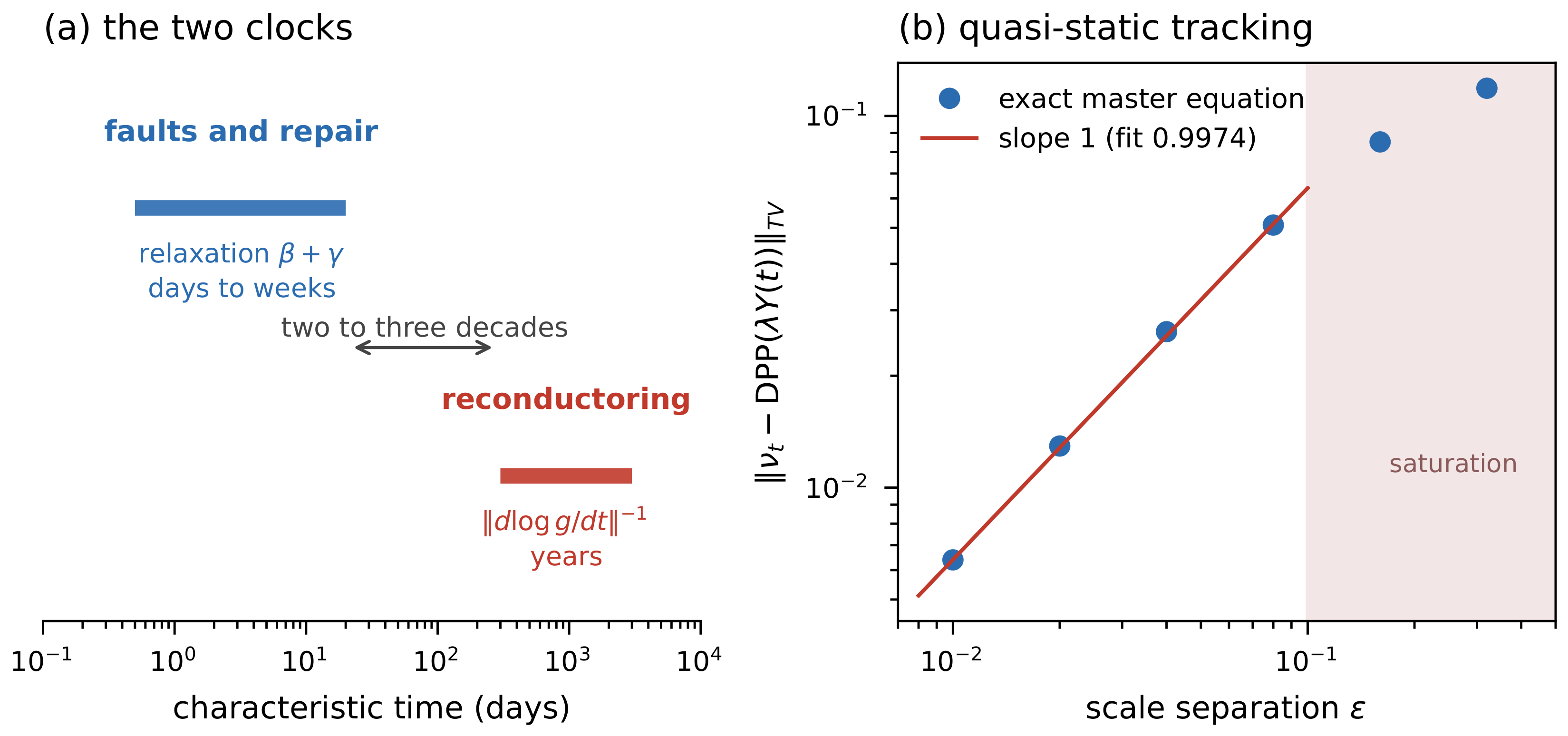
The slow layer. Estimate 1 is a scaling statement whose constant is not tracked, and a sharp adiabatic result for this family remains open. Commissioning events are jumps rather than drifts, with a transient not available in closed form.

Symmetry and radiality. The construction requires symmetric conductances and radial operation. Symmetry holds for passive line sections and fails wherever the network contains directional elements: unidirectional protection, series power-electronic devices, or any component whose impedance depends on the direction of flow. Distributed generation does not by itself break the symmetry—a passive section carries current in either direction with the same resistance—but a feeder whose protection or control makes a section usable in only one direction falls outside the model. For such networks the matrix-tree machinery must be replaced by its directed counterpart, and the electrical readings of Proposition 1 do not survive in the same form; this is the most substantial extension we leave open. Radiality is assumed throughout, so feeders operated under a weak meshed fall outside the model, a connected spanning subgraph with more than $N-1$ edges not being the basis family of a matroid.

Validation. All numerical results are computed on a published benchmark specified in full in Appendix A. This is appropriate for verifying exact identities and is not a validation against practice. What would constitute validation is an outage log from an operating utility together with the realised restoration sequences and durations, against which the diagnostic of Algorithm 1 and the indices of Corollary 2 could be compared.

Three Levels of Assertion

The results of this paper do not all require the same thing of the feeder, and conflating them is the misreading we most want to prevent. They fall into three levels, in decreasing order of robustness.

Level 1: structural quantities of the ensemble. The kernel Y and everything read off it—$Y_{ee}$ as a self transfer-current factor, the substitution map $-Y_{ef}^2$, the trace identity, the bridges, the restoration weights and their sum rule, the sensitivities of Section 7—are properties of the network and of the space of admissible configurations. They assume nothing whatever about how the feeder chooses a configuration or about what has happened to it. A feeder that has always operated one fixed radial configuration still has these quantities, and they still mean what they mean.

Level 2: occupancy quantities. The number of energised sections, the number of islands and the probability of radial completeness require that faults strike the energised sections independently and that the total restoration rate out of a k-section configuration be $\beta (r-k)$, or its time-dependent counterpart. They do not require the ensemble distribution of configurations, and by Proposition 4 they do not require any particular allocation of that rate among the candidates. They do not require the pre-fault configuration to be drawn from the ensemble: any spanning tree has exactly $N-1$ sections, so independent thinning gives $\mathrm{Bin}(N-1,p)$ energised sections and $1+\mathrm{Bin}(N-1,1-p)$ islands whichever tree the feeder happened to be operating. By Proposition 4 they do not require the canonical repair either. These are structural availability measures rather than customer-based indices (Section 5), and they are the most robust results in the paper.

Level 3: the full configuration-level law. The statement ${\nu }_t=\mathrm{DPP}\left(p\left(t\right)Y\right)$, the sector identities of Theorem 2, and the per-section and joint statements of Corollary 2 do require the initial configuration to be distributed as the operating ensemble, and they require a repair that intertwines the sectors. They do not require the canonical repair specifically: by Proposition 3 any sector intertwiner will do, and the canonical rule of Theorem 4 is the distinguished reversible member of that class. A feeder sitting in a fixed tree $T_0$ that loses one energised section is left with a uniformly chosen subset of $T_0$, not with a sample of ${\mu }_{r-1}$: Theorem 2 propagates the ensemble, it does not create it.

The ensemble is thus a description of the space of admissible configurations at Level 1, a harmless bookkeeping device at Level 2, and a genuine modelling assumption at Level 3. It never asserts that the feeder selects its configuration at random. Readers who reject the ensemble as a description of utility behaviour may still use everything at Levels 1 and 2, which is most of what an operator asks for.

11. Conclusions

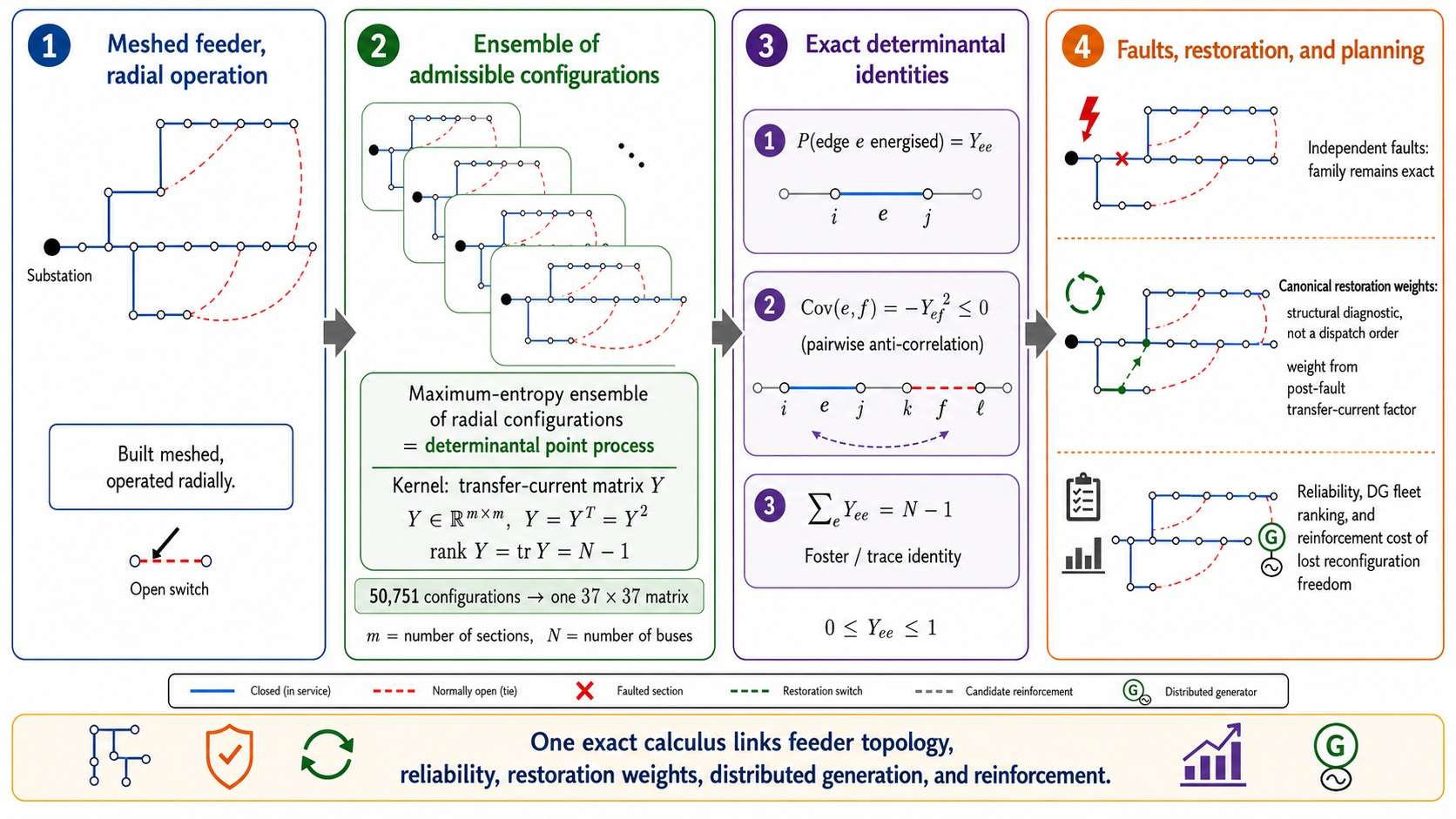
A distribution feeder operates one configuration at a time but lives in a space of them. This paper describes that space exactly. The admissible radial configurations form a determinantal ensemble whose kernel is the transfer-current matrix, so that every joint statistic of the switching devices is a small determinant rather than a sum over a combinatorial family; on the benchmark feeder this replaces an enumeration of 50,751 configurations by a single $37\times 37$ matrix, and for networks of realistic size it replaces a computation that cannot be performed at all.

Three statements summarise what the description buys, and each is exact. Random faults never take the feeder out of its model class: after any number of independent faults the surviving configuration is again a determinantal forest with the same kernel, and the relative importance profile of the sections is merely rescaled. Restoration cannot be blind, and among the mechanisms that are not blind one is canonical: no policy chosen without knowledge of the section resistances returns the feeder to its class, not even one that knows the single-line diagram in full, while conductance-aware upward intertwiners form a family of which exactly one reverses the random fault, weighting each de-energised section by its own transfer-current factor in the post-fault network with everything still energised shorted, the weights summing to the island count minus one. Its practical content is twofold and should not be overstated: it is the distinguished reversible member of the class of sector-intertwining mechanisms under which the determinantal form and the per-section indices remain exact, and the weights themselves are a structural diagnostic computed from the single-line diagram and the resistances alone. It is not a service-restoration heuristic, and Section 4.8 shows that it should not be used as one. 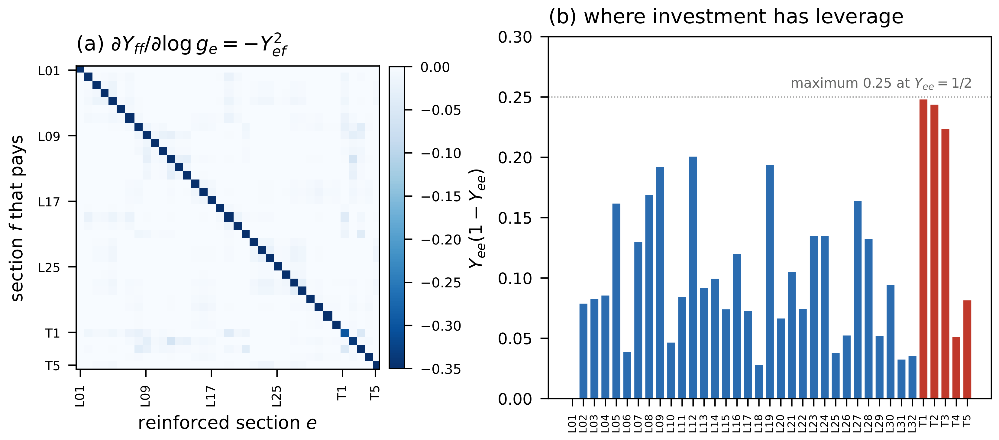Reinforcement redistributes redundancy rather than creating it: the total participation is pinned at $N-1$, the leverage of an investment is largest where the feeder is least certain, and sizing driven purely by loading spends the feeder’s switching freedom while, on the benchmark feeder, a modest redundancy term buys it back at a cost of under two per cent in loss; the threshold and the size of that penalty are properties of that network and its loading, not a general planning conclusion.

The same calculus governs a second failure layer, a fleet of distributed generators, with the projection onto the generation modes in place of the transfer-current kernel; there the restoration score of a failed unit is the residual novelty of its whitened retained-mode loading, not a gain in output variance. The contrast with the network layer is one of degree rather than of kind: the algebra alone never decides whether a canonical mechanism is also a useful rule.

What is exact and what is not should not be conflated. Everything above holds for a frozen geometry and independent faults, and the central identities were verified against exhaustive enumeration at double-precision round-off. The coupling of the two time scales is a quasi-static estimate whose constant we do not track, and the correlated events a feeder genuinely faces lie outside the distributional apparatus, though not outside the weights themselves. Section Three Levels of Assertion states which results depend on the ensemble and which do not.

Five directions follow. Validation against an operating utility’s outage log, comparing realised restoration sequences with the diagnostic of Algorithm 1, is the necessary next step and the one we have not taken. Section-specific fault rates are the assumption the model most visibly does not relax: exactness rests on uniform, blind de-energisation, and a weighted analogue would need a deletion mechanism matched to the ensemble, which we do not have. The departure from the sector law under correlated outage is measurable and exact under the null, which makes it a test statistic for whether an event was independent, computable from the switching state alone. A sharp adiabatic theorem with explicit constants would upgrade the two-scale estimate to a bound. And feeders containing directional elements require the directed counterpart of the whole construction, in which the electrical readings of Proposition 1 do not survive unchanged.