Peristalsis of Thermally Heated Eyring–Powell Fluid Within an Elliptic Channel Having Ciliated Wavy Walls Under Mass Transfer Impact

Abstract

The physical characteristics of a heated non-Newtonian Eyring–Powell fluid in a conduit with sinusoidally moving ciliated walls are highlighted in this analytical study. The impact of mass transmission is considered in this model. The dimensional form of the governing equations is simplified using the long-wavelength estimation and suitable transformations to produce a set of dimensionless partial differential equations with pertinent boundary conditions. To solve it, the perturbation technique is utilized applying polynomial solutions. The solutions of temperature, concentrations, and velocity profiles are obtained, and then are further analyzed through graphical results. An accurate mathematical solution for the pressure gradient is achieved by integrating the velocity profile over the elliptic cross-section. The non-Newtonian Eyring–Powell fluid flows quicker through this vertical ciliated elliptic duct than the Newtonian fluid. Moreover, the cilia elliptic movement eccentricity and the wave number for metachronal wave have a dual effect on the velocity profile. Increasing the dimensionless flow rate and occlusion leads to an increase in closed contour size, as seen in the streamline description.

1. Introduction

Combining mathematical study of cilia-generated transient waves and peristaltic flow is a highly interesting issue. From tiny creatures like bacteria to bigger animals, cilia are found in a wide variety of biological systems. Their biological processes such as protozoa swimming, cilia beating in epithelial cells, and cilia rotating in mouse nodes determine how they move. Cells and other creatures’ surfaces have tiny, hair-like structures called cilia. Cilia play a crucial part in functions including breathing, circulation, movement, and the passage of food through the digestive tract [1], and they are found in practically every animal kingdom. An enhanced model of the cilia-developed flow inside tubes was mathematically examined by Blake [2]. The mathematical study of heat transfer and fluid movement within a cylindrical tube with ciliated and sinusoidally deformable walls was conducted by Akbar and Khan [3]. The model of mathematics that explains the heat transfer of a non-Newtonian fluid via a tube with ciliated walls was introduced by Akbar and Butt [4]. Many scholars use different geometrical models, such as asymmetric ciliated channels [5], a cylindrical shape with ciliated walls [6], curved pipes with ciliated walls [7], and micro-channels through metachronal waves of cilia [8], to quantitatively evaluate the peristaltic flow analysis combined with ciliated walls effect. Through a tapered, ciliated, symmetric porous tube, Imran et al. [9] took into account electroosmosis, and viscoelastic fluid is transported peristaltically in curved ducts with ciliated walls in the article of Abbasi et al. [10].

Several researchers also interpret the transmission of heat and mass for peristaltic motion issues while taking into account the different geometrical and non-Newtonian models. In a rectangular cross-section tube, Hafez et al. [11] investigate the effects of heat and mass transmission for Casson fluid over an inclined plane with rotation, while Hafez et al. [12] investigate the effects of very small solid particles and magnetism in a fluid that is porous. Various techniques have been presented in the literature for different fluids of the thermodynamic models on this topic, such as in the articles [13,14,15,16,17].

Numerous research publications explore peristaltic flow in various geometries, including cylinders, asymmetric channels, and rectangular ducts. Despite its significant industrial and technical uses, peristaltic flow inside elliptical ducts has received little mathematical attention. Researchers are increasingly interested in the computational interpretation of convection in elliptic conduits because of their huge applications. Elliptic ducts have a higher heat transfer coefficient compared to circular ducts. Elliptical ducts often have lower drag forces than circular ducts. Additionally, an elliptic duct has a lower pressure drop than a circular one. The results of an elliptical duct are the same as those of a circular one if their cross-sectional areas are equal [18]. Many mathematical studies described the peristaltic motion through an elliptical duct in the presence of heat transmission, such as Saleem et al. [19] for Casson fluid flow, Nadeem et al. [20] for Jeffrey fluid flow, Akhtar et al. [21] for Newtonian viscous fluid with single-wall carbon nanotubes, and Rachid et al. [22], taking into account the physical quantities of entropy generation and mechanical efficiency. In an elliptic conduit, a hybrid nanofluid moved peristaltically with entropy production and heat transfer (McCash et al. [23]) and with elasticity (Devaki [24]). The effect of a peristaltically occurring fluid in a Rabinowitsch fluid model on the elliptic duct and fluctuating liquid characteristics was examined by Nadeem et al. [25]. Based on the results of the convective heat transport study in [25], Akhtar et al. [26] carried out their investigation. Carreau fluid’s peristaltic flow via an oval cross-sectional conduit was studied by Shahzad et al. [27]. For a Prandtl fluid model, Shahzad et al. [28] also used the same methodology. The investigations [29,30,31,32] applied the same technique for heated ciliated walls in various fluids. The combined heat and mass transfer for peristaltic movement in a duct with an elliptic cross-section has been the subject of recent research [33,34,35,36].

Researchers are increasingly interested in the peristaltic flow of various non-Newtonian fluids due to their wide range of applications. Among these non-Newtonian fluids is Eyring–Powell fluid, which is the subject of our study in this research. There are many studies that consider this fluid in different ducts like a cylindrical pipe (Akbar and Nadeem [37]), a rectangular tube (Hayat et al. [38]), a curved channel (Abassi et al. [39]; Hina et al. [40,41]), and an elliptical duct (Awan et al. [42]; Akram et al. [43]; Shahzad et al. [44]; Hafez et al. [45]).

In this study, the mathematical model that explains the peristaltic movement of non-Newtonian Erying–Powell fluid in the elliptical channel with ciliated walls will be revealed for the first time. Our goal is to explain the peristaltic flow mechanism within a ciliated elliptic duct because the existing literature mainly discusses peristalsis activity for ciliated cylindrical, asymmetric channels, etc. Furthermore, cilia are present in several mammal species and are essential to numerous biological propulsion processes, as can be seen if we take a biological perspective. It is also not required that every biological structure have a circular cross-section; for example, an upper ureter’s cross-section is more appropriately thought of as elliptic. The temperature, concentration, and velocity profiles are obtained by solving the partial differential equations that represent the problem using the perturbation technique and the fourth-degree polynomial.

2. Mathematical Formulation

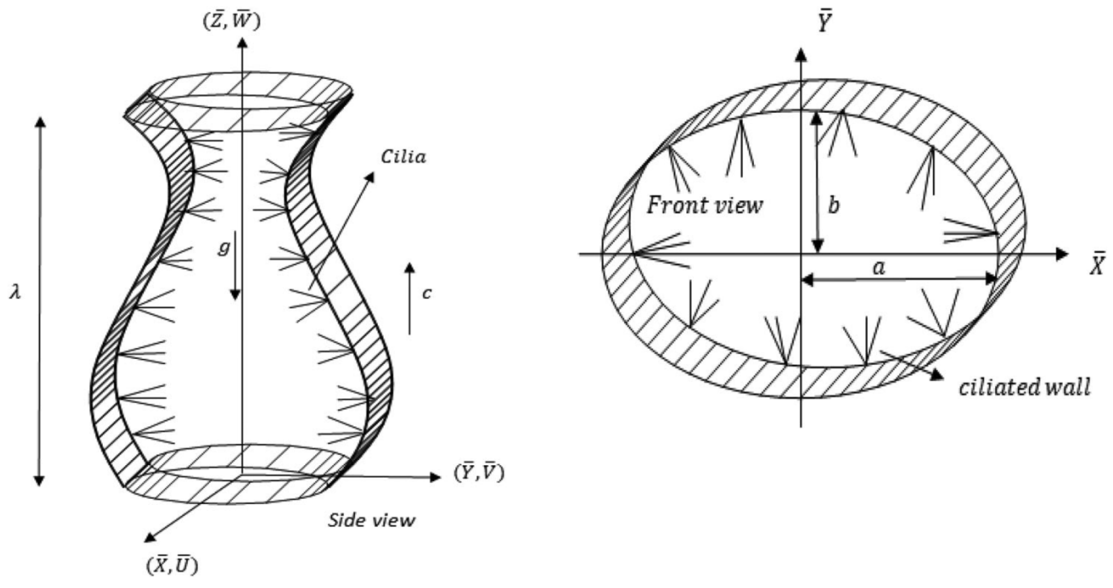
The peristaltic motion of Eyring–Powell fluid in a vertical conduit which has an elliptic cross section and ciliated walls is mathematically explored in Figure 1. The mass and heat transmission are taken into account. An elliptical conduit with ciliated sinusoidal walls can be represented geometrically as [29,30,31,32]:

$$\begin{array}{cc}\hfill \tilde{Y}& =b_0+\delta \cos \left[{\displaystyle \frac{2\pi }{\lambda }}\left(\tilde{Z}-c\tilde{t}\right)\right]=\tilde{f}\left(\tilde{Z},\tilde{t}\right)\hfill \\ \hfill \tilde{Z}& ={\tilde{Z}}_0+\delta \epsilon \sin \left[{\displaystyle \frac{2\pi }{\lambda }}\left(\tilde{Z}-c\tilde{t}\right)\right]=\tilde{g}\left(\tilde{Z},{\tilde{Z}}_0,\tilde{t}\right)\hfill \end{array}$$

(1)

where $a_0$ and $b_0$ represent the elliptic duct’s semi-major and semi-minor axes, respectively; $\delta$ represents the wave amplitude; $\lambda$ represents the wavelength and $\tilde{t}$ represents the wave time; c represents the speed of sinusoidal waves traveling; and $\epsilon$ represents the cilia elliptic movement eccentricity.

Additionally, cilia tip velocity is represented mathematically as [29,30,31,32]:

$$\begin{array}{cc}\hfill \tilde{W}& ={\left.{\displaystyle \frac{\partial \tilde{Z}}{\partial \tilde{t}}}\right|}_{{\tilde{Z}}_0}={\displaystyle \frac{\partial \tilde{g}}{\partial \tilde{t}}}+{\displaystyle \frac{\partial \tilde{g}}{\partial \tilde{Z}}}{\displaystyle \frac{\partial \tilde{Z}}{\partial \tilde{t}}}={\displaystyle \frac{\partial \tilde{g}}{\partial \tilde{t}}}+{\displaystyle \frac{\partial \tilde{g}}{\partial \tilde{Z}}}\tilde{W}\hfill \\ \hfill \tilde{V}& ={\left.{\displaystyle \frac{\partial \tilde{Y}}{\partial \tilde{t}}}\right|}_{{\tilde{Z}}_0}={\displaystyle \frac{\partial \tilde{f}}{\partial \tilde{t}}}+{\displaystyle \frac{\partial \tilde{f}}{\partial \tilde{Z}}}{\displaystyle \frac{\partial \tilde{Z}}{\partial \tilde{t}}}={\displaystyle \frac{\partial \tilde{f}}{\partial \tilde{t}}}+{\displaystyle \frac{\partial \tilde{f}}{\partial \tilde{Z}}}\tilde{W}\hfill \end{array}$$

(2)

Combining Equations (1) and (2) result in

$$\begin{array}{cc}\hfill \tilde{W}& ={\displaystyle \frac{-\frac{2\pi }{\lambda }\left(\delta \epsilon c\cos \left[\frac{2\pi }{\lambda }\left(\tilde{Z}-c\tilde{t}\right)\right]\right)}{1-\frac{2\pi }{\lambda }\left(\delta \epsilon \cos \left[\frac{2\pi }{\lambda }\left(\tilde{Z}-c\tilde{t}\right)\right]\right)}}\hfill \\ \hfill \tilde{V}& ={\displaystyle \frac{\frac{2\pi }{\lambda }\left(\delta c\sin \left[\frac{2\pi }{\lambda }\left(\tilde{Z}-c\tilde{t}\right)\right]\right)}{1-\frac{2\pi }{\lambda }\left(\delta \epsilon \cos \left[\frac{2\pi }{\lambda }\left(\tilde{Z}-c\tilde{t}\right)\right]\right)}}\hfill \end{array}$$

(3)

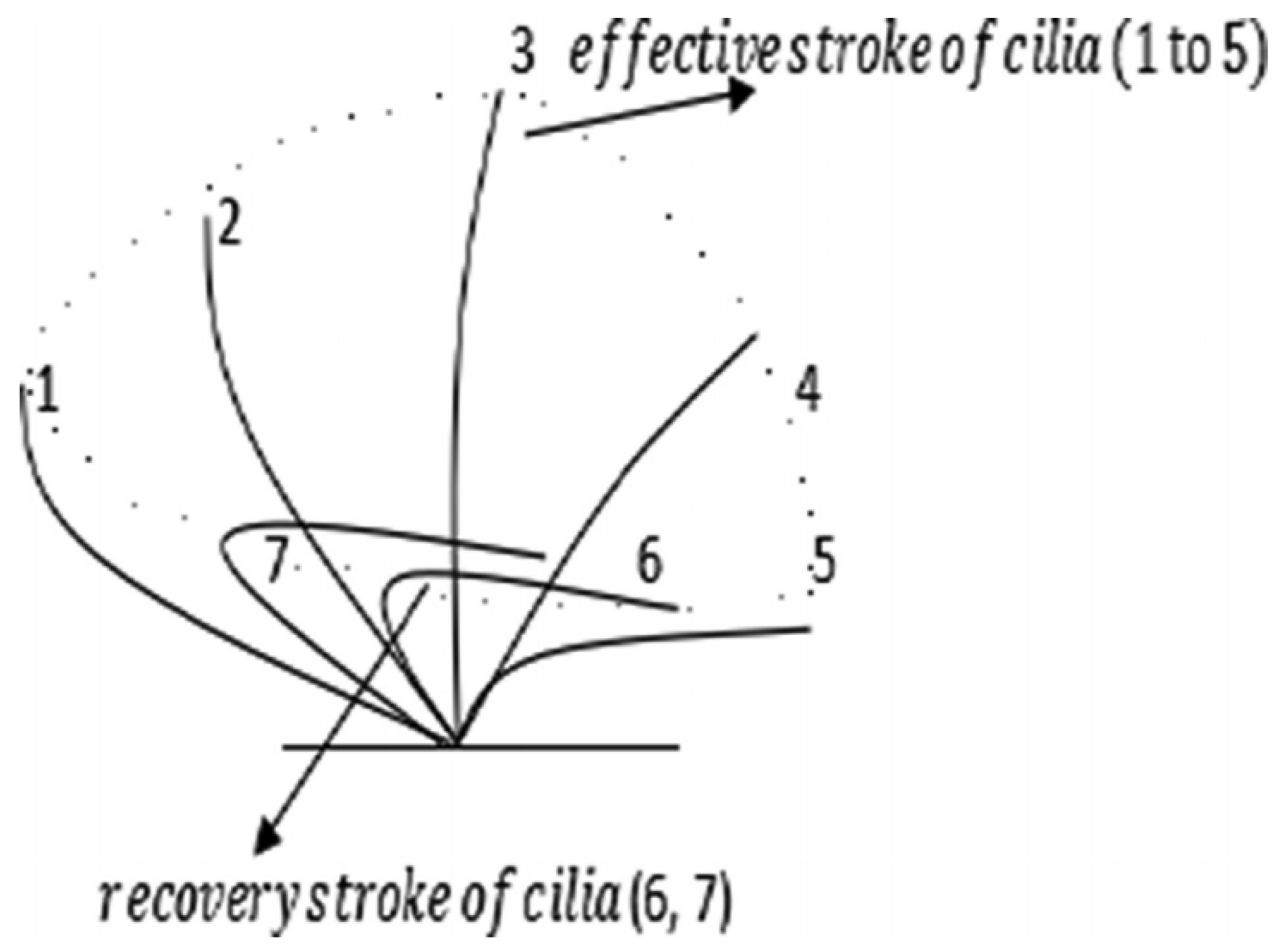
Here, the two velocity formulas ($\tilde{W}$ and $\tilde{V}$) differentiate between the cilia’s effective and recovery strokes. For a full cycle of efficient and recuperative strokes, the movement of cilia tips (shown in Figure 2) is seen as an elliptical route movement. It is clear that the cilia freely retreats close to the conduit surface throughout its recuperative stroke but stays firm during its efficient stroke.

Below are the governing equations that account for the motion of a non-Newtonian, incompressible Erying–Powell fluid in an elliptic conduit, providing estimations for heat and mass transmission [34,36].

$${\nabla }_{·}\overrightarrow{V}=0$$

(4)

$$\rho {\displaystyle \frac{d\overrightarrow{V}}{dt}}=-\nabla \tilde{P}+{\nabla }_{·}\overrightarrow{\tilde{S}}-\rho \left[{\gamma }_T\left(\tilde{T}-{\tilde{T}}_W\right)+{\gamma }_C\left(\tilde{C}-{\tilde{C}}_W\right)\right]\overrightarrow{g}$$

(5)

$$\rho c_p{\displaystyle \frac{d\tilde{T}}{dt}}=\kappa {\nabla }^2\tilde{T}+\tilde{\mathsf{\Gamma }}$$

(6)

$${\displaystyle \frac{d\tilde{C}}{dt}}=D^{*}{\nabla }^2\tilde{C}+{\displaystyle \frac{D^{*}{K}_T}{T_b}}{\nabla }^2\tilde{T}$$

(7)

where $\rho$ is the density of the fluid, $\tilde{P}$ is the pressure, $\overrightarrow{\tilde{S}}$ denotes the extra stress tensor for Eyring–Powell fluid, $\overrightarrow{g}$ is the gravity acceleration, $\tilde{T}$ is the fluid temperature, $c_p$ is the specific heat, $\kappa$ is the thermal conductivity, $\tilde{\mathsf{\Gamma }}$ is the heat source/sink parameter, $\tilde{C}$ is the fluid concentration, $D^{*}$ is the coefficient of mass diffusivity, $K_T$ is the thermal diffusion ratio, $T_b$ is the mean fluid temperature, ${\tilde{T}}_W$ is the duct wall temperature, ${\tilde{C}}_W$ is the duct wall concentration, and ${\gamma }_T$, ${\gamma }_C$ are the thermal and concentration expansion coefficients, respectively.

Using the non-Newtonian Eyring–Powell fluid model, the study’s related extra stress tensor is given by [38]

$$\overrightarrow{\tilde{S}}=\mu \nabla \overrightarrow{V}+{\displaystyle \frac{1}{{\beta }_1}}{\sinh }^{-1}\left({\displaystyle \frac{\nabla \overrightarrow{V}}{c_1}}\right)$$

(8)

where ${\beta }_1$ and $c_1$ are the Eyring–Powell fluid’s material constants and $\mu$ is the dynamic viscosity. The second-order approximation is used to estimate the term ${\sinh }^{-1}$ as

$${\sinh }^{-1}\left({\displaystyle \frac{\nabla \overrightarrow{V}}{c_1}}\right)\cong {\displaystyle \frac{\nabla \overrightarrow{V}}{c_1}}-{\displaystyle \frac{1}{6}}{\left({\displaystyle \frac{\nabla \overrightarrow{V}}{c_1}}\right)}^3\mathrm{for}\left|{\displaystyle \frac{\nabla \overrightarrow{V}}{c_1}}\right|\ll 1$$

(9)

Equations (4)–(7) can be rewritten as [36,42]

$${\displaystyle \frac{\partial \tilde{U}}{\partial \tilde{X}}}+{\displaystyle \frac{\partial \tilde{V}}{\partial \tilde{Y}}}+{\displaystyle \frac{\partial \tilde{W}}{\partial \tilde{Z}}}=0$$

(10)

$$\begin{array}{cc}\hfill \rho \left({\displaystyle \frac{\partial \tilde{U}}{\partial \tilde{t}}}+\tilde{U}{\displaystyle \frac{\partial \tilde{U}}{\partial \tilde{X}}}+\tilde{V}{\displaystyle \frac{\partial \tilde{U}}{\partial \tilde{Y}}}+\tilde{W}{\displaystyle \frac{\partial \tilde{U}}{\partial \tilde{Z}}}\right)& =-{\displaystyle \frac{\partial \tilde{P}}{\partial \tilde{X}}}+{\displaystyle \frac{\partial {\tilde{S}}_{\tilde{X}\tilde{X}}}{\partial \tilde{X}}}+{\displaystyle \frac{\partial {\tilde{S}}_{\tilde{X}\tilde{Y}}}{\partial \tilde{Y}}}+{\displaystyle \frac{\partial {\tilde{S}}_{\tilde{X}\tilde{Z}}}{\partial \tilde{Z}}}\hfill \end{array}$$

(11)

$$\begin{array}{cc}\hfill \rho \left({\displaystyle \frac{\partial \tilde{V}}{\partial \tilde{t}}}+\tilde{U}{\displaystyle \frac{\partial \tilde{V}}{\partial \tilde{X}}}+\tilde{V}{\displaystyle \frac{\partial \tilde{V}}{\partial \tilde{Y}}}+\tilde{W}{\displaystyle \frac{\partial \tilde{V}}{\partial \tilde{Z}}}\right)=-{\displaystyle \frac{\partial \tilde{P}}{\partial \tilde{Y}}}+{\displaystyle \frac{\partial {\tilde{S}}_{\tilde{Y}\tilde{X}}}{\partial \tilde{X}}}+{\displaystyle \frac{\partial {\tilde{S}}_{\tilde{Y}\tilde{Y}}}{\partial \tilde{Y}}}& +{\displaystyle \frac{\partial {\tilde{S}}_{\tilde{Y}\tilde{Z}}}{\partial \tilde{Z}}}\hfill \end{array}$$

(12)

$$\begin{array}{cc}\hfill \rho \left({\displaystyle \frac{\partial \tilde{W}}{\partial \tilde{t}}}+\tilde{U}{\displaystyle \frac{\partial \tilde{W}}{\partial \tilde{X}}}+\tilde{V}{\displaystyle \frac{\partial \tilde{W}}{\partial \tilde{Y}}}+\tilde{W}{\displaystyle \frac{\partial \tilde{W}}{\partial \tilde{Z}}}\right)& =-{\displaystyle \frac{\partial \tilde{P}}{\partial \tilde{Z}}}+{\displaystyle \frac{\partial {\tilde{S}}_{\tilde{Z}\tilde{X}}}{\partial \tilde{X}}}+{\displaystyle \frac{\partial {\tilde{S}}_{\tilde{Z}\tilde{Y}}}{\partial \tilde{Y}}}+{\displaystyle \frac{\partial {\tilde{S}}_{\tilde{Z}\tilde{Z}}}{\partial \tilde{Z}}}\hfill \\ \hfill & +\rho {\gamma }_{T}g\left(\tilde{T}-{\tilde{T}}_W\right)+\rho {\gamma }_{C}g\left(\tilde{C}-{\tilde{C}}_W\right)\hfill \end{array}$$

(13)

$$\begin{array}{cc}\hfill \rho c_p\left({\displaystyle \frac{\partial \tilde{T}}{\partial \tilde{t}}}+\tilde{U}{\displaystyle \frac{\partial \tilde{T}}{\partial \tilde{X}}}+\tilde{V}{\displaystyle \frac{\partial \tilde{T}}{\partial \tilde{Y}}}+\tilde{W}{\displaystyle \frac{\partial \tilde{T}}{\partial \tilde{Z}}}\right)& =\kappa \left({\displaystyle \frac{{\partial }^2\tilde{T}}{\partial {\tilde{X}}^2}}+{\displaystyle \frac{{\partial }^2\tilde{T}}{\partial {\tilde{Y}}^2}}+{\displaystyle \frac{{\partial }^2\tilde{T}}{\partial {\tilde{Z}}^2}}\right)+\tilde{\mathsf{\Gamma }}\hfill \end{array}$$

(14)

$$\begin{array}{cc}\hfill {\displaystyle \frac{\partial \tilde{C}}{\partial \tilde{t}}}+\tilde{U}{\displaystyle \frac{\partial \tilde{C}}{\partial \tilde{X}}}+\tilde{V}{\displaystyle \frac{\partial \tilde{C}}{\partial \tilde{Y}}}+\tilde{W}{\displaystyle \frac{\partial \tilde{C}}{\partial \tilde{Z}}}& =D^{*}\left({\displaystyle \frac{{\partial }^2\tilde{C}}{\partial {\tilde{X}}^2}}+{\displaystyle \frac{{\partial }^2\tilde{C}}{\partial {\tilde{Y}}^2}}+{\displaystyle \frac{{\partial }^2\tilde{C}}{\partial {\tilde{Z}}^2}}\right)\hfill \\ \hfill & +{\displaystyle \frac{D^{*}{K}_T}{T_b}}\left({\displaystyle \frac{{\partial }^2\tilde{T}}{\partial {\tilde{X}}^2}}+{\displaystyle \frac{{\partial }^2\tilde{T}}{\partial {\tilde{Y}}^2}}+{\displaystyle \frac{{\partial }^2\tilde{T}}{\partial {\tilde{Z}}^2}}\right)\hfill \end{array}$$

(15)

The dimensional form of the associated boundary conditions for an elliptic duct with ciliated walls is shown as [31]

$$\begin{array}{cc}\hfill \tilde{W}& ={\displaystyle \frac{-\frac{2\pi }{\lambda }\left(\delta \epsilon c\cos \left[\frac{2\pi }{\lambda }\left(\tilde{Z}-c\tilde{t}\right)\right]\right)}{1-\frac{2\pi }{\lambda }\left(\delta \epsilon \cos \left[\frac{2\pi }{\lambda }\left(\tilde{Z}-c\tilde{t}\right)\right]\right)}},\hfill \\ \hfill \tilde{T}& ={\tilde{T}}_W,\tilde{C}={\tilde{C}}_W\mathrm{at}{\displaystyle \frac{{\tilde{X}}^2}{{\tilde{a}}^2}}+{\displaystyle \frac{{\tilde{Y}}^2}{{\tilde{b}}^2}}=1\hfill \end{array}$$

(16)

The following transformations are used to change the current issue from an unstable flow model to a steady-flow model [33,34,35,36]:

$$\begin{array}{cc}\hfill \tilde{x}& =\tilde{X},\tilde{y}=\tilde{Y},\tilde{z}=\tilde{Z}-c\tilde{t},\tilde{u}=\tilde{U},\tilde{\upsilon }=\tilde{V},\hfill \\ \hfill \tilde{w}& =\tilde{W}-c,\tilde{p}=\tilde{P},\tilde{T}=T,\tilde{C}=C\hfill \end{array}$$

(17)

The non-dimensional quantities included in this study are as follows [33,34,35,36]:

$$\begin{array}{cc}\hfill x& ={\displaystyle \frac{\tilde{x}}{{\tilde{D}}_h}},y={\displaystyle \frac{\tilde{y}}{{\tilde{D}}_h}},z={\displaystyle \frac{\tilde{z}}{\lambda }},t={\displaystyle \frac{c\tilde{t}}{\lambda }},u={\displaystyle \frac{\lambda \tilde{u}}{{\tilde{D}}_{h}c}},\upsilon ={\displaystyle \frac{\lambda \tilde{\upsilon }}{{\tilde{D}}_{h}c}},w={\displaystyle \frac{\tilde{w}}{c}},\hfill \\ \hfill p& ={\displaystyle \frac{{\tilde{D}}_h^2\tilde{p}}{c\mu \lambda }},\mathsf{\Theta }={\displaystyle \frac{\tilde{T}-{\tilde{T}}_W}{{\tilde{T}}_b-{\tilde{T}}_W}},\chi ={\displaystyle \frac{\tilde{C}-{\tilde{C}}_W}{{\tilde{C}}_b-{\tilde{C}}_W}},ϵ={\displaystyle \frac{b_0}{a_0}},S_{ij}={\displaystyle \frac{{\tilde{D}}_h{\tilde{S}}_{ij}}{\mu c}},\hfill \\ \hfill \mathrm{Re}& ={\displaystyle \frac{\rho c{\tilde{D}}_h}{\mu }},a={\displaystyle \frac{\tilde{a}}{{\tilde{D}}_h}},b={\displaystyle \frac{\tilde{b}}{{\tilde{D}}_h}},\varphi ={\displaystyle \frac{\delta }{b_0}},{\sigma }_T={\displaystyle \frac{\rho {\gamma }_{T}g\left({\tilde{T}}_b-{\tilde{T}}_W\right){\tilde{D}}_h^2}{\mu c}},\hfill \\ \hfill {\sigma }_C& ={\displaystyle \frac{\rho {\gamma }_{C}g\left({\tilde{C}}_b-{\tilde{C}}_W\right){\tilde{D}}_h^2}{\mu c}},\mathrm{{\rm Y}}={\displaystyle \frac{\tilde{\mathsf{\Gamma }}{\tilde{D}}_h^2}{\kappa \left({\tilde{T}}_b-{\tilde{T}}_W\right)}},Sr={\displaystyle \frac{\rho D^{*}{K}_T\left({\tilde{T}}_b-{\tilde{T}}_W\right)}{\mu T_b\left({\tilde{C}}_b-{\tilde{C}}_W\right)}},\hfill \\ \hfill Sc& ={\displaystyle \frac{\mu }{\rho D^{*}}},\beta ={\displaystyle \frac{1}{\mu {\beta }_1{c}_1}},\alpha ={\displaystyle \frac{\beta }{6}}{\left({\displaystyle \frac{c}{c_1{\tilde{D}}_h}}\right)}^2,\xi ={\displaystyle \frac{b_0}{\lambda }},\hfill \end{array}$$

(18)

where the bulk temperature is denoted by ${\tilde{T}}_b$ and the concentration by ${\tilde{C}}_b$. The Reynolds number, thermal Grashof’s number, concentration Grashof’s number, heat source parameter, Soret number, Schmidt number, and occlusion are represented by the non-dimensional parameters Re, ${\sigma }_T$, ${\sigma }_C$, $\mathrm{{\rm Y}}$, $Sr$, $Sc$, and $\varphi$, respectively. The Eyring–Powell fluid’s dimensionless properties are denoted by the values $\beta$ and $\alpha$. The wave number for metachronal wave is denoted by $\xi$.

To take into consideration buoyant forces resulting from temperature and concentration gradients, the thermal and solutal Grashof numbers are included; however, it is assumed that these effects are minor and do not cause inertial dominance in the flow. The Grashof numbers are insufficient to refute the Stokes-flow assumption. As a result, buoyancy appears as a weak driving force that modifies the viscous-dominated flow without changing its underlying creeping-flow characteristics.

The idea of hydraulic diameter must be taken into account whenever we work with a non-circular domain. It is calculated by dividing the wetted cross-sectional perimeter by four times the cross-sectional area. For the ellipse, the hydraulic diameter ${\tilde{D}}_h$ is specified as [42,43,44]

$${\tilde{D}}_h={\displaystyle \frac{b_0\pi }{E\left(\varrho \right)}}$$

(19)

The eccentricity of an ellipse, indicated by $\varrho$, ranges from 0 to 1, and is denoted by

$$\varrho =\sqrt{1-{ϵ}^2}$$

(20)

Then, $E\left(\varrho \right)$ may be expressed mathematically as [29,30,31,32,33,34,35,36]

$$E\left(\varrho \right)={\displaystyle \underset{0}{\overset{\pi /2}{\int }}}\sqrt{1-{\varrho }^2{\sin }^2\left(\eta \right)}d\eta$$

(21)

The characteristic wavelength of the metachronal wave is usually significantly larger than the channel height or duct width in many biological systems where cilia-driven transport is seen. The long-wavelength approximation (i.e., $\lambda \gg h$), which simplifies the governing equations by ignoring higher-order axial changes, is justified by this difference in scales. Similarly, because of the tiny characteristic length scales (e.g., cilia length on the order of 5–10 μm) and low flow velocities typically in the range of (≈10–100 μm/s), the Reynolds number in such systems is often quite small ($\mathrm{Re}\ll 1$). The localized velocity gradients are introduced close to the walls due to the presence of cilia and metachronal waves. Nevertheless, these effects are limited to a narrow area next to the border, and the imposed boundary conditions that describe the wave motion adequately capture their averaged influence. As a result, the lubrication framework continues to accurately characterize the bulk flow. Moreover, the small Reynolds number ($\mathrm{Re}\ll 1$) means that inertial effects in momentum equations are minimal relative to viscous forces, supporting the creeping-flow assumption. Equations (10)–(15) use the transformations given in Equation (17) and the dimensionless values supplied in Equation (18) under the assumption of a lower Reynolds number ($\mathrm{Re}\ll 1$) and long wavelength ($\lambda ⟶\infty$). The dimensionless formulation of the resulting equations is described as

$${\displaystyle \frac{\partial p}{\partial x}}=0$$

(22)

$${\displaystyle \frac{\partial p}{\partial y}}=0$$

(23)

$${\displaystyle \frac{dp}{dz}}={\displaystyle \frac{\partial S_{zx}}{\partial x}}+{\displaystyle \frac{\partial S_{zy}}{\partial y}}+{\sigma }_T\mathsf{\Theta }+{\sigma }_C\chi$$

(24)

$${\displaystyle \frac{{\partial }^2\mathsf{\Theta }}{\partial x^2}}+{\displaystyle \frac{{\partial }^2\mathsf{\Theta }}{\partial y^2}}+\mathrm{{\rm Y}}=0$$

(25)

$${\displaystyle \frac{{\partial }^2\chi }{\partial x^2}}+{\displaystyle \frac{{\partial }^2\chi }{\partial y^2}}+SrSc\left({\displaystyle \frac{{\partial }^2\mathsf{\Theta }}{\partial x^2}}+{\displaystyle \frac{{\partial }^2\mathsf{\Theta }}{\partial y^2}}\right)=0$$

(26)

The respective boundary conditions in the non-dimensional formulation are obtained as [31]:

$$w=\mathsf{\Omega },\mathsf{\Theta }=0,\chi =0\mathrm{at}{\displaystyle \frac{x^2}{a^2}}+{\displaystyle \frac{y^2}{b^2}}=1$$

(27)

in which

$$\begin{array}{cc}\hfill \mathsf{\Omega }& =-1-{\displaystyle \frac{2\pi \varphi \xi \epsilon \cos \left[2\pi z\right]}{1-2\pi \varphi \xi \epsilon \cos \left[2\pi z\right]}}\hfill \\ \hfill a& ={\displaystyle \frac{E\left(\varrho \right)}{\pi }}\left({\displaystyle \frac{1}{ϵ}}+\varphi \sin \left(2\pi z\right)\right)\mathrm{and}b={\displaystyle \frac{E\left(\varrho \right)}{\pi }}\left(1+\varphi \sin \left(2\pi z\right)\right)\hfill \end{array}$$

(28)

Here, Equations (8) and (9) are used to get the stress components of the Eyring–Powell fluid displayed below [42]:

$$S_{zx}=\left(1+\beta \right){\displaystyle \frac{\partial w}{\partial x}}-\alpha {\left({\displaystyle \frac{\partial w}{\partial x}}\right)}^3$$

(29)

$$S_{zy}=\left(1+\beta \right){\displaystyle \frac{\partial w}{\partial y}}-\alpha {\left({\displaystyle \frac{\partial w}{\partial y}}\right)}^3$$

(30)

Consequently, Equations (29) and (30) in Equation (24), yield

$$\begin{array}{cc}\hfill {\displaystyle \frac{dp}{dz}}& =\left(1+\beta \right)\left({\displaystyle \frac{{\partial }^{2}w}{\partial x^2}}+{\displaystyle \frac{{\partial }^{2}w}{\partial y^2}}\right)-3\alpha \left[{\left({\displaystyle \frac{\partial w}{\partial x}}\right)}^2{\displaystyle \frac{{\partial }^{2}w}{\partial x^2}}+{\left({\displaystyle \frac{\partial w}{\partial y}}\right)}^2{\displaystyle \frac{{\partial }^{2}w}{\partial y^2}}\right]\hfill \\ \hfill & +{\sigma }_T\mathsf{\Theta }+{\sigma }_C\chi \hfill \end{array}$$

(31)

3. Technique of Solutions

3.1. Solutions of Temperature and Concentration

To get the precise mathematical solution for the temperature profile using the same technique described in [46], we take into account the following polynomial expression:

$$\mathsf{\Theta }\left(x,y,z\right)={\widehat{B}}_1{x}^4+{\widehat{B}}_2{y}^4+{\widehat{B}}_3{x}^2{y}^2+{\widehat{B}}_4{x}^2+{\widehat{B}}_5{y}^2+{\widehat{B}}_6$$

(32)

When Equation (32) is entered into Equation (25), and after comparing the coefficients of $x^2$, $y^2$, $x^0$, $y^0$, it produces

$$6{\widehat{B}}_1+{\widehat{B}}_3=0$$

(33)

$$6{\widehat{B}}_2+{\widehat{B}}_3=0$$

(34)

$$2{\widehat{B}}_4+2{\widehat{B}}_5+\mathrm{{\rm Y}}=0$$

(35)

Equation (32) is substituted for temperature in boundary condition (27), and the coefficients of $x^4$, $x^2$, $x^0$ on both sides are compared to obtain

$$a^4{\widehat{B}}_1+b^4{\widehat{B}}_2-a^2{b}^2{\widehat{B}}_3=0$$

(36)

$$-2b^4{\widehat{B}}_2+a^2{b}^2{\widehat{B}}_3+a^2{\widehat{B}}_4-b^2{\widehat{B}}_5=0$$

(37)

$$b^4{\widehat{B}}_2+b^2{\widehat{B}}_5+{\widehat{B}}_6=0$$

(38)

These constant terms are obtained by simultaneously solving the previously indicated set of Equations (33)–(38), and they are given as

$${\widehat{B}}_1={\widehat{B}}_2={\widehat{B}}_3=0,{\widehat{B}}_4={\displaystyle \frac{-\mathrm{{\rm Y}}{b}^2}{2\left(a^2+b^2\right)}},{\widehat{B}}_5={\displaystyle \frac{-\mathrm{{\rm Y}}{a}^2}{2\left(a^2+b^2\right)}},{\widehat{B}}_6={\displaystyle \frac{\mathrm{{\rm Y}}{a}^2{b}^2}{2\left(a^2+b^2\right)}}$$

(39)

The temperature solution was derived by inserting the quantities of constants from Equation (39), as follows, into Equation (32):

$$\mathsf{\Theta }\left(x,y,z\right)={\displaystyle \frac{-\mathrm{{\rm Y}}}{2\left(a^2+b^2\right)}}\left(b^2{x}^2+a^2{y}^2-a^2{b}^2\right)$$

(40)

Equation (26) is evaluated using the relevant boundary condition provided in Equation (27). To acquire the precise concentration solution, we first apply the temperature solution from Equation (40) to Equation (26) and then utilize the same polynomial solution technique in Equation (32)

$$\chi \left(x,y,z\right)={\displaystyle \frac{\mathrm{{\rm Y}}SrSc}{2\left(a^2+b^2\right)}}\left(b^2{x}^2+a^2{y}^2-a^2{b}^2\right)$$

(41)

3.2. Solution of Axial Velocity

The associated temperature (40) and concentration (41) solutions are incorporated in momentum Equation (31), which can then be solved by employing a polynomial perturbation technique and utilizing $\alpha$ as the perturbation parameter. Consider that

$$\begin{array}{cc}\hfill w& =w_0+\alpha w_1+\dots \dots \dots \dots \dots \hfill \end{array}$$

(42)

$$\begin{array}{cc}\hfill p& =p_0+\alpha p_1+\dots \dots \dots \dots \dots \hfill \end{array}$$

(43)

$$\begin{array}{cc}\hfill Q& =Q_0+\alpha Q_1+\dots \dots \dots \dots \dots \hfill \end{array}$$

(44)

where Q represents the time-averaged volume flow rate. Equations (42) and (43) are substituted in Equation (31) and boundary condition (27) to generate the following system of equations for the velocity function by comparing the coefficients of ${\left(\alpha \right)}^0$ and ${\left(\alpha \right)}^1$ and disregarding greater exponents.

3.2.1. Solution of Zeroth-Order ${\left(\alpha \right)}^0$ System

$${\displaystyle \frac{d{p}_0}{dz}}=\left(1+\beta \right)\left({\displaystyle \frac{{\partial }^2{w}_0}{\partial x^2}}+{\displaystyle \frac{{\partial }^2{w}_0}{\partial y^2}}\right)-{\displaystyle \frac{\mathrm{{\rm Y}}\left({\sigma }_T-{\sigma }_{C}SrSc\right)}{2\left(a^2+b^2\right)}}\left(b^2{x}^2+a^2{y}^2-a^2{b}^2\right)$$

(45)

$$w_0=\mathsf{\Omega }\mathrm{at}{\displaystyle \frac{x^2}{a^2}}+{\displaystyle \frac{y^2}{b^2}}=1$$

(46)

The following fourth-degree polynomial can be used to solve Equation (45) with the first condition in Equation (46)

$$w_0\left(x,y,z\right)={\tilde{B}}_1{x}^4+{\tilde{B}}_2{y}^4+{\tilde{B}}_3{x}^2{y}^2+{\tilde{B}}_4{x}^2+{\tilde{B}}_5{y}^2+{\tilde{B}}_6$$

(47)

After substituting Equation (47) into Equation (45), and comparing the coefficients of $x^2$, $y^2$, and the constant terms, we get

$$(\beta +1)\left(12{\tilde{B}}_1+2{\tilde{B}}_3\right)-{\displaystyle \frac{\left(b^2\mathrm{{\rm Y}}\right)\left({\sigma }_T-ScSr{\sigma }_C\right)}{2\left(a^2+b^2\right)}}=0$$

(48)

$$(\beta +1)\left(12{\tilde{B}}_2+2{\tilde{B}}_3\right)-{\displaystyle \frac{\left(a^2\mathrm{{\rm Y}}\right)\left({\sigma }_T-ScSr{\sigma }_C\right)}{2\left(a^2+b^2\right)}}=0$$

(49)

$$(\beta +1)\left(2{\tilde{B}}_4+2{\tilde{B}}_5\right)+{\displaystyle \frac{\left(a^2{b}^2\mathrm{{\rm Y}}\right)\left({\sigma }_T-ScSr{\sigma }_C\right)}{2\left(a^2+b^2\right)}}={\displaystyle \frac{d{p}_0}{dz}}$$

(50)

Comparing equivalent powers of x and applying Equation (47) to the boundary condition in Equation (46), we arrive at

$$a^4{\tilde{B}}_1-a^2{b}^2{\tilde{B}}_3+b^4{\tilde{B}}_2=0$$

(51)

$$a^2{b}^2{\tilde{B}}_3+a^2{\tilde{B}}_4-2b^4{\tilde{B}}_2-b^2{\tilde{B}}_5=0$$

(52)

$$b^4{\tilde{B}}_2+b^2{\tilde{B}}_5+{\tilde{B}}_6=\mathsf{\Omega }$$

(53)

The values of the constants ${\tilde{B}}_1$–${\tilde{B}}_6$, which are given in the “Appendix A,” are obtained by concurrently solving Equations (48)–(53). Equation (47) thus becomes

$$\begin{array}{cc}\hfill w_0\left(x,y,z\right)& =\mathsf{\Omega }-{\displaystyle \frac{\left(a^2(b-y)(b+y)-b^2{x}^2\right)}{24(\beta +1){\left(a^2+b^2\right)}^2\left(a^4+6a^2{b}^2+b^4\right)}}\hfill \\ \hfill & \begin{array}{c}\left(12{\displaystyle \frac{d{p}_0}{dz}}\left(a^2+b^2\right)\left(a^4+6a^2{b}^2+b^4\right)+\mathrm{{\rm Y}}\left(ScSr{\sigma }_C-{\sigma }_T\right)\right.\\ \begin{array}{c}\left(b^2\left(5a^2+b^2\right)\left(a^4-x^2\left(a^2+b^2\right)+5a^2{b}^2\right)\right.\\ \left.\left.-a^2{y}^2\left(a^2+b^2\right)\left(a^2+5b^2\right)\right)\right)\end{array}\end{array}\hfill \end{array}$$

(54)

The volumetric flow rate is obtained by integrating Equation (54) throughout the elliptical cross-section as

$$q_0\left(z\right)={\displaystyle \frac{\pi ab\left(12\mathsf{\Omega }(\beta +1){\left(a^2+b^2\right)}^2-a^4{b}^4\mathrm{{\rm Y}}\left(ScSr{\sigma }_C-{\sigma }_T\right)-3a^2{b}^2\frac{d{p}_0}{dz}\left(a^2+b^2\right)\right)}{12(\beta +1){\left(a^2+b^2\right)}^2}}$$

(55)

The following formula can be used to determine the pressure gradient:

$${\displaystyle \frac{d{p}_0}{dz}}={\displaystyle \frac{4(\beta +1)\left(a^2+b^2\right)\left(\pi ab\mathsf{\Omega }-\frac{\pi a^5{b}^5\mathrm{{\rm Y}}\left(ScSr{\sigma }_C-{\sigma }_T\right)}{12(\beta +1){\left(a^2+b^2\right)}^2}+L-Q_0\right)}{\pi a^3{b}^3}}$$

(56)

in which

$$L={\displaystyle \underset{0}{\overset{1}{\int }}}abdz={\displaystyle \frac{{\left(E\left(\varrho \right)\right)}^2(2+ϵ{\varphi }^2)}{2{\pi }^2ϵ}}$$

3.2.2. Solution of First-Order ${\left(\alpha \right)}^1$ System

$${\displaystyle \frac{d{p}_1}{dz}}=\left(1+\beta \right)\left({\displaystyle \frac{{\partial }^2{w}_1}{\partial x^2}}+{\displaystyle \frac{{\partial }^2{w}_1}{\partial y^2}}\right)-3\left[{\left({\displaystyle \frac{\partial w_0}{\partial x}}\right)}^2{\displaystyle \frac{{\partial }^2{w}_0}{\partial x^2}}+{\left({\displaystyle \frac{\partial w_0}{\partial y}}\right)}^2{\displaystyle \frac{{\partial }^2{w}_0}{\partial y^2}}\right]$$

(57)

$$w_1=0\mathrm{at}{\displaystyle \frac{x^2}{a^2}}+{\displaystyle \frac{y^2}{b^2}}=1$$

(58)

The system solution of Equations (57) and (58) was obtained by using a similar process to that used to solve the zeroth-order system of Equations (45) and (46) as follows:

$$\begin{array}{cc}\hfill w_1\left(x,y,z\right)& =-{\displaystyle \frac{\left(a^2(b-y)(b+y)-b^2{x}^2\right)}{2(\beta +1)\left(a^2+b^2\right)\left(a^4+6a^2{b}^2+b^4\right)}}\{{\displaystyle \frac{d{p}_1}{dz}}\left(a^4+6a^2{b}^2+b^4\right)\hfill \\ \hfill & +4{\tilde{B}}_5^3\left(y^2\left(a^2+b^2\right)\left(a^2+6b^2\right)+b^2\left(a^4-x^2\left(a^2+b^2\right)+5a^2{b}^2\right)\right)\hfill \\ \hfill & +4{\tilde{B}}_4^3\left(a^4\left(5b^2+6x^2-y^2\right)+a^2{b}^2\left(b^2+7x^2-y^2\right)+b^4{x}^2\right)\}\hfill \end{array}$$

(59)

$$q_1\left(z\right)=-{\displaystyle \frac{\pi a^3{b}^3\left(4a^2{\tilde{B}}_4^3+4b^2{\tilde{B}}_5^3+\frac{d{p}_1}{dz}\right)}{4(\beta +1)\left(a^2+b^2\right)}}$$

(60)

$${\displaystyle \frac{d{p}_1}{dz}}=-{\displaystyle \frac{4\left(\pi a^5{b}^3{\tilde{B}}_4^3+\pi a^3{b}^5{\tilde{B}}_5^3+(\beta +1)\left(a^2+b^2\right)\left(Q_1-L\right)\right)}{\pi a^3{b}^3}}$$

(61)

As a result, the final form of velocity and pressure gradient are ultimately:

$$\begin{array}{cc}\hfill w\left(x,y,z\right)& =\mathsf{\Omega }+{\displaystyle \frac{\left(a^2(b-y)(b+y)-b^2{x}^2\right)}{864(\beta +1){\left(a^2+b^2\right)}^2{\left(a^4+6a^2{b}^2+b^4\right)}^4}}\{-36\mathrm{{\rm Y}}{\left(a^4+6a^2{b}^2+b^4\right)}^3\hfill \\ \hfill & \left(b^2\left(5a^2+b^2\right)\left(a^4-x^2\left(a^2+b^2\right)+5a^2{b}^2\right)-a^2{y}^2\left(a^2+b^2\right)\left(a^2+5b^2\right)\right)\left(ScSr{\sigma }_C-{\sigma }_T\right)\hfill \\ \hfill & -432{\displaystyle \frac{dp}{dz}}\left(a^2+b^2\right){\left(a^4+6a^2{b}^2+b^4\right)}^4-{\displaystyle \frac{\alpha }{{\pi }^3{a}^9{b}^9{(\beta +1)}^3{\left(a^2+b^2\right)}^2}}\hfill \\ \hfill & \begin{array}{c}\left(b^6\left(a^4\left(5b^2+6x^2-y^2\right)+a^2{b}^2\left(b^2+7x^2-y^2\right)+b^4{x}^2\right)\right.\\ \begin{array}{c}\left(\pi a^5{b}^5\mathrm{{\rm Y}}\left(3a^2+b^2\right)\left(ScSr{\sigma }_C-{\sigma }_T\right)\right.\\ {\left.+24(\beta +1)\left(a^2+b^2\right)\left(a^4+6a^2{b}^2+b^4\right)(L-Q)\right)}^3\end{array}\\ +a^6\left(y^2\left(a^2+b^2\right)\left(a^2+6b^2\right)+b^2\left(a^4-x^2\left(a^2+b^2\right)+5a^2{b}^2\right)\right)\\ \left.\begin{array}{c}\left(\pi a^5{b}^5\mathrm{{\rm Y}}\left(a^2+3b^2\right)\left(ScSr{\sigma }_C-{\sigma }_T\right)\right.\\ {\left.+24(\beta +1)\left(a^2+b^2\right)\left(a^4+6a^2{b}^2+b^4\right)(L-Q)\right)}^3\end{array}\right)\end{array}\}\hfill \end{array}$$

(62)

$$\begin{array}{cc}\hfill {\displaystyle \frac{dp}{dz}}& ={\displaystyle \frac{4(\beta +1)\left(a^2+b^2\right)}{\pi a^3{b}^3}}\{\alpha L+ab\pi \mathsf{\Omega }+L-Q+{\displaystyle \frac{\pi a^5{b}^5}{1728(\beta +1){\left(a^2+b^2\right)}^2}}\hfill \\ \hfill & \{-{\displaystyle \frac{\alpha }{{\pi }^3{a}^9{b}^9{(\beta +1)}^3{\left(a^2+b^2\right)}^2{\left(a^4+6a^2{b}^2+b^4\right)}^3}}\hfill \\ \hfill & \begin{array}{c}\begin{array}{c}\left(a^4\left(\pi a^5{b}^5\mathrm{{\rm Y}}\left(a^2+3b^2\right)\left(ScSr{\sigma }_C-{\sigma }_T\right)\right.\right.\\ {\left.+24(\beta +1)\left(a^2+b^2\right)\left(a^4+6a^2{b}^2+b^4\right)(L-Q)\right)}^3\end{array}\\ \begin{array}{c}+b^4\left(\pi a^5{b}^5\mathrm{{\rm Y}}\left(3a^2+b^2\right)\left(ScSr{\sigma }_C-{\sigma }_T\right)\right.\\ \left.{\left.+24(\beta +1)\left(a^2+b^2\right)\left(a^4+6a^2{b}^2+b^4\right)(L-Q)\right)}^3\right)\end{array}\end{array}\hfill \\ \hfill & -144ScSr\mathrm{{\rm Y}}{\sigma }_C+144\mathrm{{\rm Y}}{\sigma }_T\left\}\right\}\hfill \end{array}$$

(63)

The mathematical expressions for the pressure rise and frictional force for a single wavelength are

$$\mathsf{\Delta }P={\displaystyle \underset{0}{\overset{1}{\int }}}{\displaystyle \frac{\partial p}{\partial z}}dz$$

(64)

$$\mathsf{\Delta }F=-{\displaystyle \underset{0}{\overset{1}{\int }}}ab{\displaystyle \frac{\partial p}{\partial z}}dz$$

(65)

4. Validity of Results

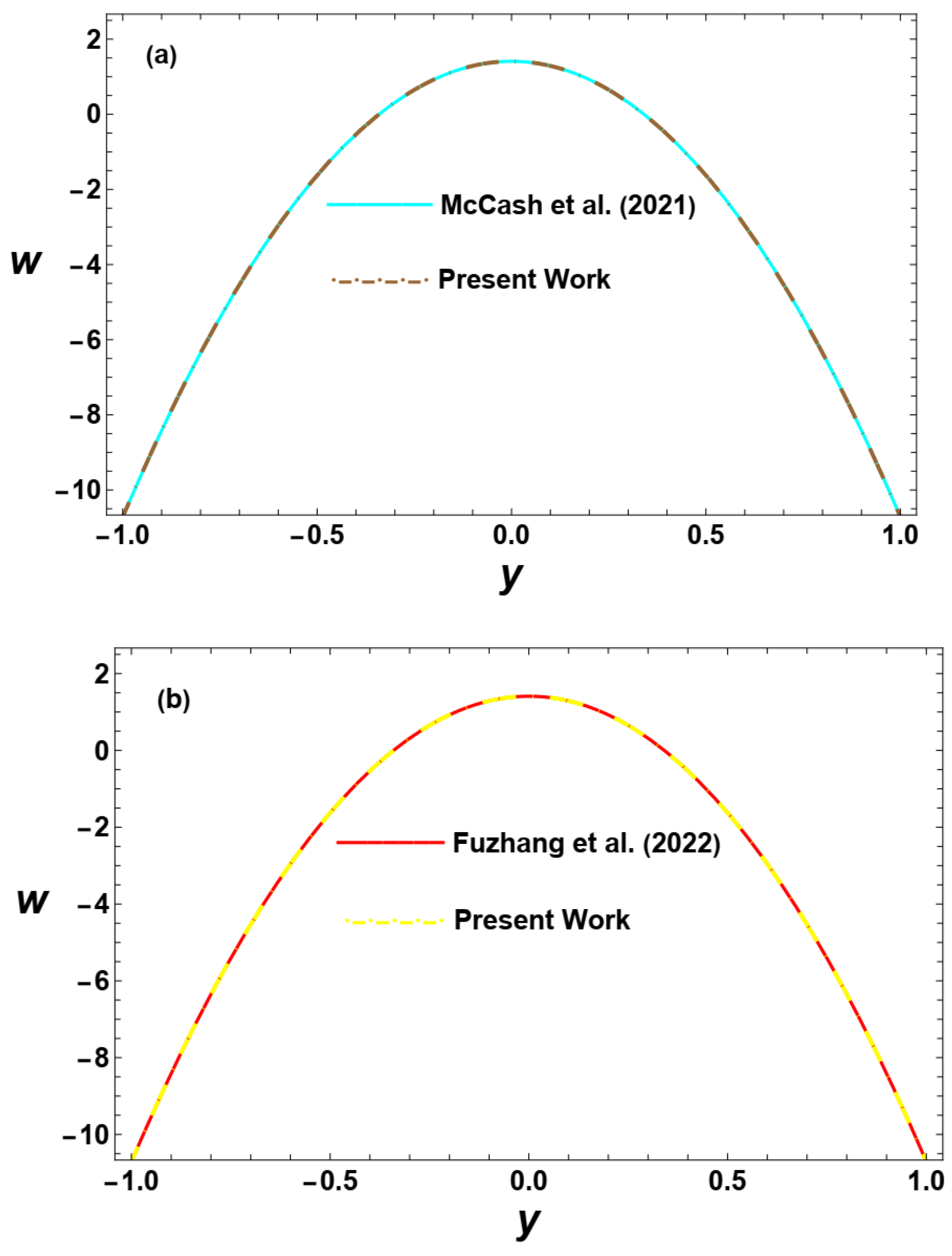
The validity of the analytical findings from the preceding part is assessed in this section. For $\alpha =0$, and $\beta =0$, which reflect the study of Newtonian fluid flow, our results agree with those in the studies [29,33] without ciliated walls ($\mathsf{\Omega }=0$). A graphical validation of these findings is shown in Figure 3a. When the constant $\alpha$ vanishes, the constant $\beta$ is replaced by its reciprocal, which is considered the Casson constant; our results are limited to those of [31] if $\alpha ={\sigma }_C=0$ and [34] if $\mathsf{\Omega }=0$, demonstrating a strong agreement in Figure 3b. In the paper of Awan et al. [42], the same axial velocity is obtained for a constant flow down a stenotic vein with an elliptic cross-section for $\mathsf{\Omega }={\sigma }_T={\sigma }_C=0$ by considering blood as an Erying–Powell fluid, and similar to those obtained by Akram et al. [43] without nanoparticles. When the walls are non-ciliated ($\mathsf{\Omega }=0$), the current study aligns with Hafez et al. [45], and excellent agreement with the results was observed. These discussed comparisons show that including Eyring–Powell fluid model behavior causes noticeable differences in flow resistance and pumping characteristics compared to the Newtonian case, whereas the presence of cilia significantly improves transport efficiency due to the extra momentum provided by metachronal wave motion.

Comparison with Circular Ciliated Duct

• Setting semi-axes equal ($a=b$) yields the axial velocity of a circular cross-section duct for Eyring–Powell fluid peristaltic flow.
• When $a=b$ and $\alpha =\beta =0$, these outcomes correspond to the peristaltic movement of Newtonian fluid via the circular duct.

5. Results and Discussion

This study examines the effects of mass and heat transmission on the Eyring–Powell fluid through a ciliated elliptical conduit. This section alters flow-included parameters numerically to study the outcomes of temperature, concentration, velocity, and pressure gradient fields via both two-dimensional (2D) and three-dimensional (3D) graphical representations, with Figures (a) in Figure 4, Figure 5, Figure 6, Figure 7, Figure 8, Figure 9, Figure 10, Figure 11, Figure 12, Figure 13 and Figure 14 illustrating 2D results and Figures (b) in Figure 4, Figure 5, Figure 6, Figure 7, Figure 8, Figure 9, Figure 10, Figure 11, Figure 12, Figure 13 and Figure 14 showing 3D results. Additionally, the pressure rise impact and trapping phenomenon of bolus are provided in the current section.

5.1. Temperature and Concentration Profiles

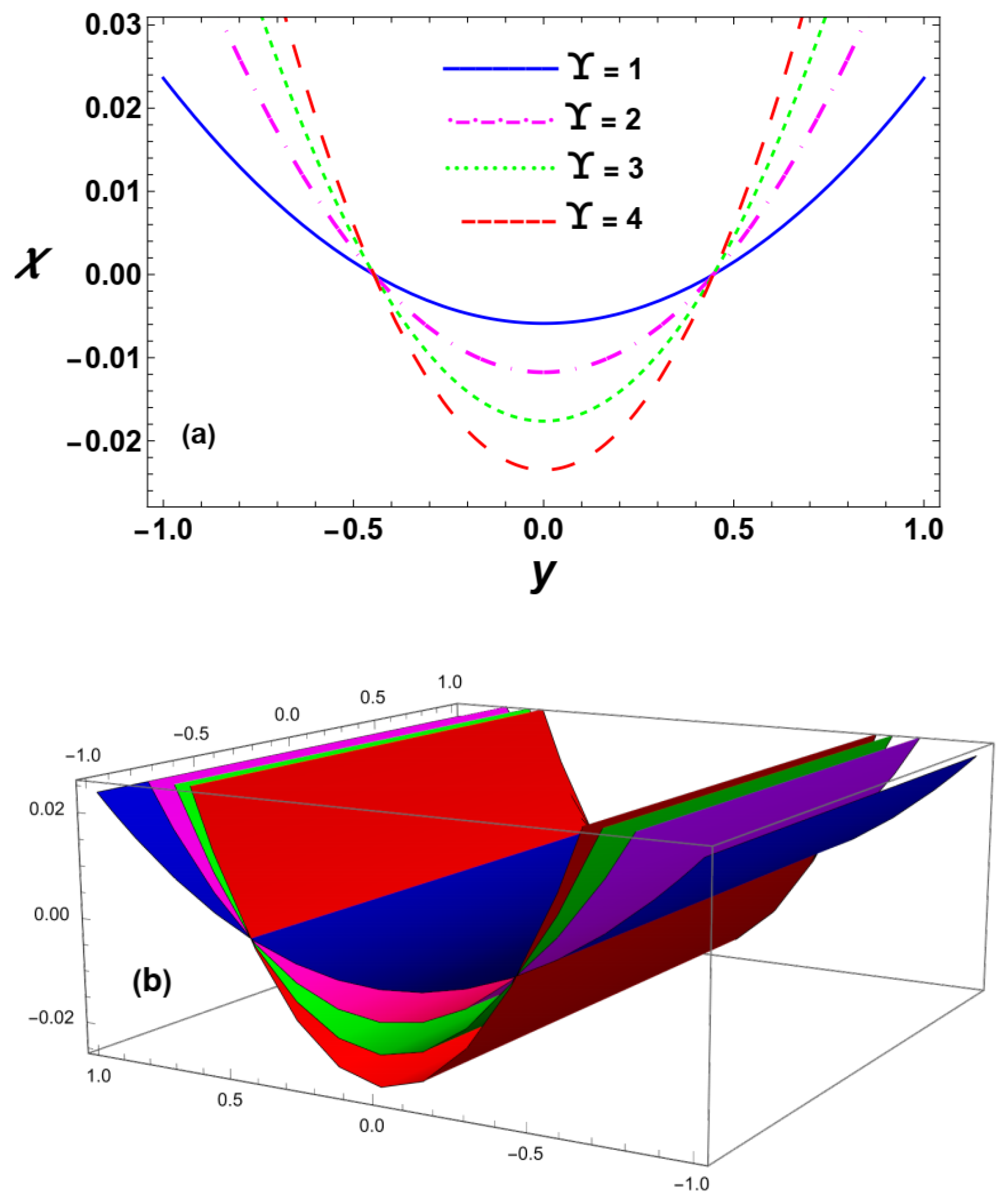
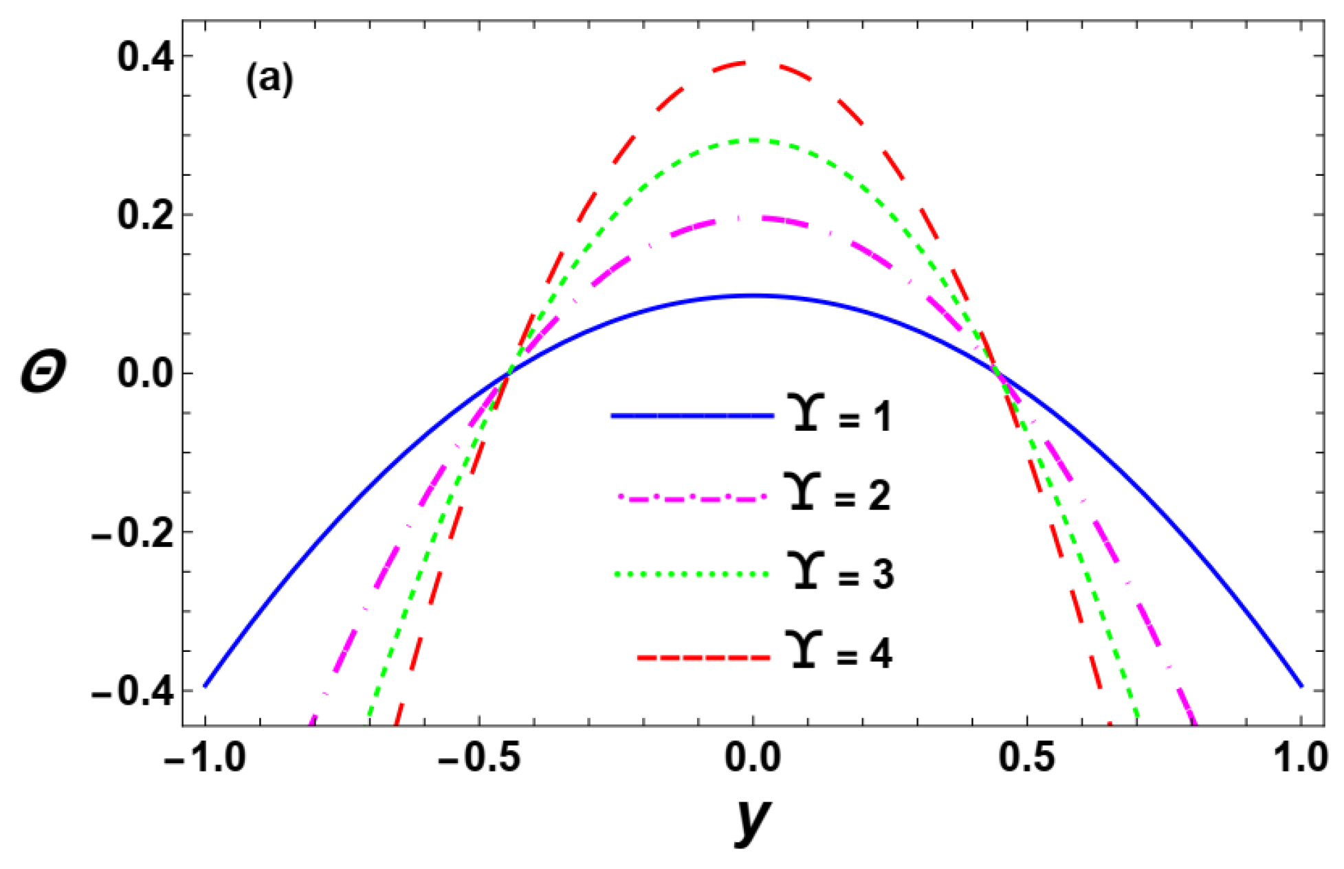
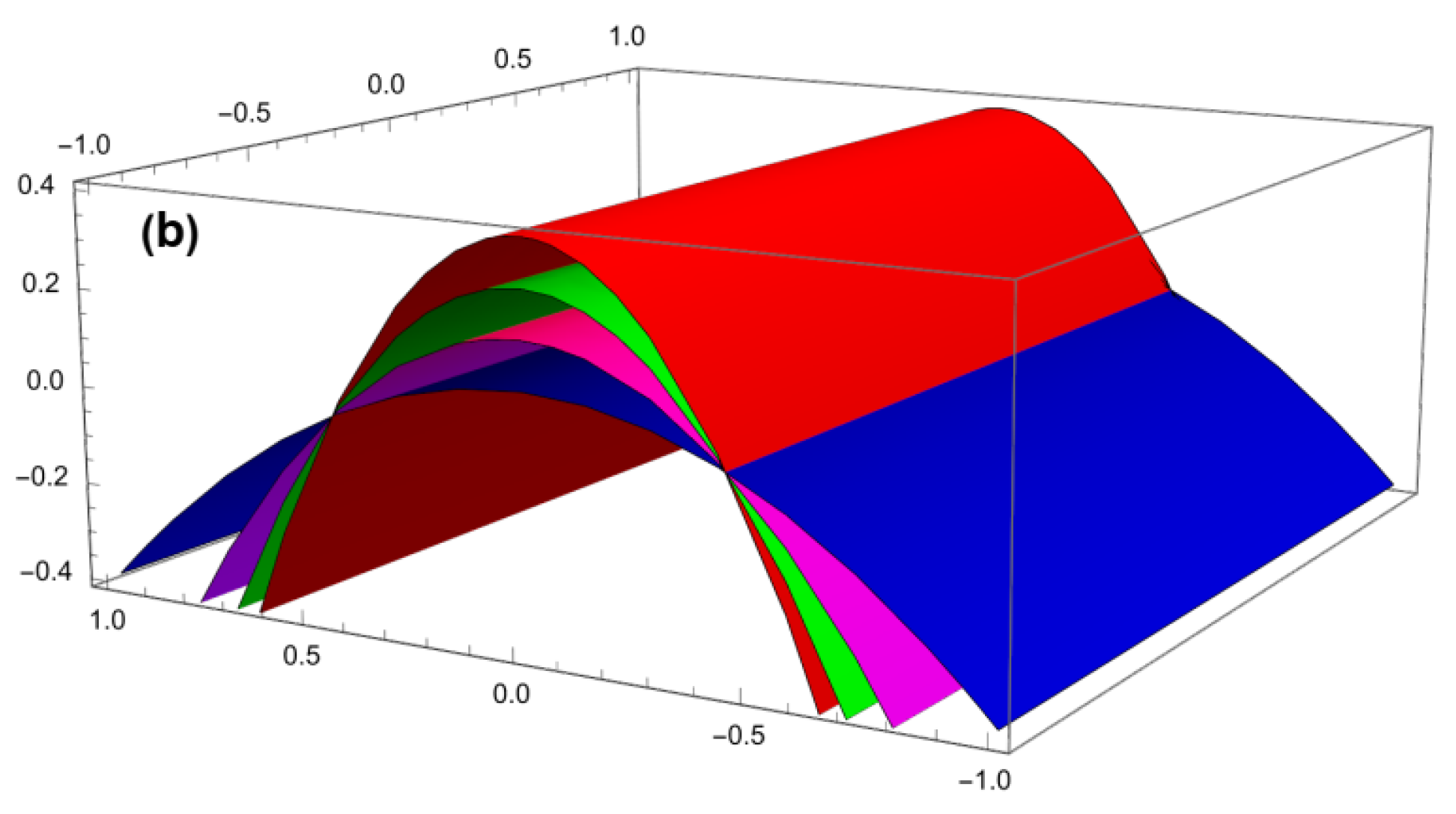
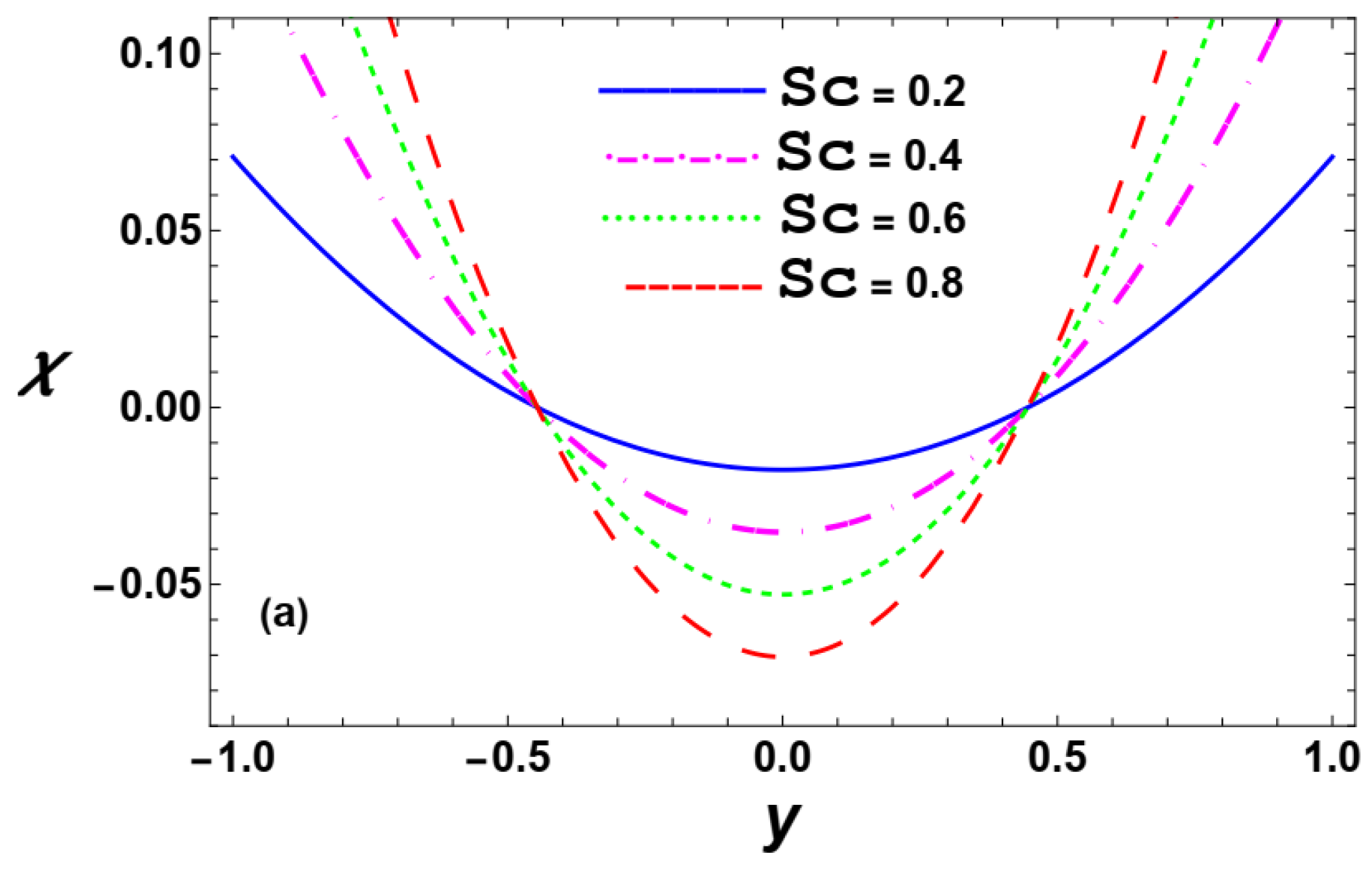
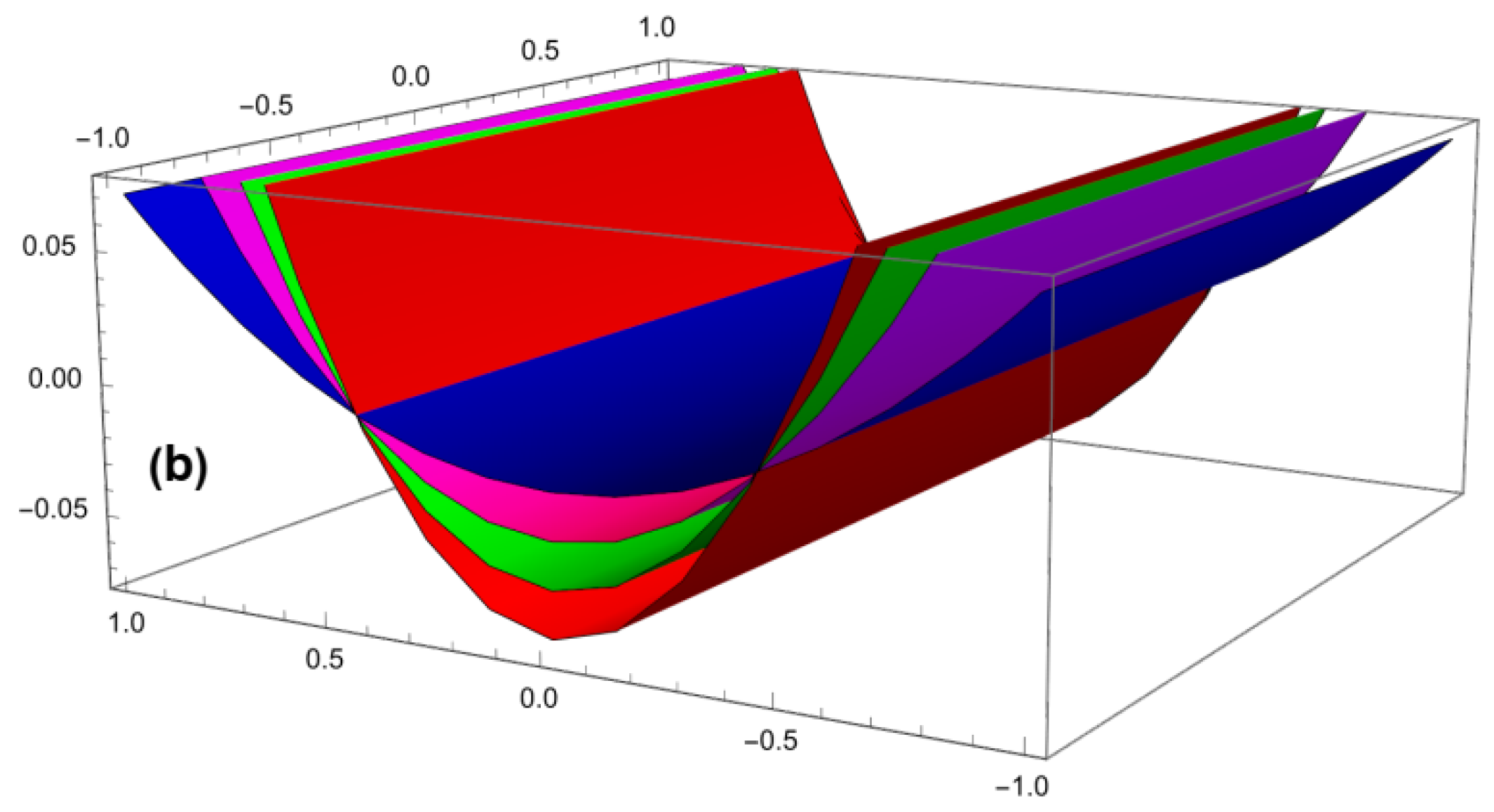
Temperature and concentration for the associated problem parameters are shown graphically in Figure 4, Figure 5 and Figure 6. The temperature and concentration profiles’s graphic shapes for rising heat absorption values $\mathrm{{\rm Y}}$ in 2D and 3D, respectively, are shown in Figure 4 and Figure 5. It is seen from Figure 4a,b that the temperature profile decreases at the channel’s outside wall, while rising in the middle due to the increase in the parameter value $\mathrm{{\rm Y}}$. The temperature graphs have a parabolic pattern along the axis, which is noteworthy. An axially symmetric temperature profile is seen for this elliptic duct. Furthermore, the temperature steadily decreases toward the ciliated walls after reaching its maximum in the elliptic duct’s center. For both 2D and 3D graphical findings, Figure 5a,b show how the dimensionless parameter $\mathrm{{\rm Y}}$ affects the concentration field, which has the opposite impact than the temperature field. This pattern makes intuitive sense from a physics standpoint, given that heat and mass are diametrically opposed. Figure 6a,b depict the impact of Schmidt number $Sc$ on the concentration difference, which is also affected by parameter $\mathrm{{\rm Y}}$, indicating a decrease in mass diffusivity and an increase in kinematic viscosity; increasing $Sc$ resulted in a decrease in concentration. It was discovered that the Soret number $Sr$ has the same effect on the distribution of concentrations as parameter $Sc$, but the corresponding figures are not given here to avoid any kind of repetition. Because the Soret number is inversely proportional to the concentration difference, an increase in $Sr$ value leads to a decrease in concentration.

Figure 4. Variation in temperature profile $\mathsf{\Theta }$ given by Equation (40), with y for different values of $\mathrm{{\rm Y}}$. (a) Two-dimensional profile; (b) Three-dimensional profile, if, $ϵ=0.1$, $\varphi =0.4$, $x=0.01$, $z=0.2$, $\xi =0.1$, $\epsilon =0.1$, when $\mathrm{{\rm Y}}=1$, 2, 3, and 4, respectively.

Figure 4. Variation in temperature profile $\mathsf{\Theta }$ given by Equation (40), with y for different values of $\mathrm{{\rm Y}}$. (a) Two-dimensional profile; (b) Three-dimensional profile, if, $ϵ=0.1$, $\varphi =0.4$, $x=0.01$, $z=0.2$, $\xi =0.1$, $\epsilon =0.1$, when $\mathrm{{\rm Y}}=1$, 2, 3, and 4, respectively.

Figure 5. Variation in concentration profile $\chi$ given by Equation (41), with y for different values of $\mathrm{{\rm Y}}$. (a) Two-dimensional profile; (b) Three-dimensional profile, if, $ϵ=0.1$, $\varphi =0.4$, $Sr=0.3$, $Sc=0.2$, $Q=2$, $x=0.01$, $z=0.2$, $\xi =0.1$, $\epsilon =0.1$, when $\mathrm{{\rm Y}}=1$, 2, 3, and 4, respectively.

Figure 5. Variation in concentration profile $\chi$ given by Equation (41), with y for different values of $\mathrm{{\rm Y}}$. (a) Two-dimensional profile; (b) Three-dimensional profile, if, $ϵ=0.1$, $\varphi =0.4$, $Sr=0.3$, $Sc=0.2$, $Q=2$, $x=0.01$, $z=0.2$, $\xi =0.1$, $\epsilon =0.1$, when $\mathrm{{\rm Y}}=1$, 2, 3, and 4, respectively.

Figure 6. Variation in concentration profile $\chi$ given by Equation (41), with y for different values of $Sc$. (a) Two-dimensional profile; (b) Three-dimensional profile, if, $ϵ=0.1$, $\varphi =0.4$, $\mathrm{{\rm Y}}=3$, $Sr=0.3$, $Q=2$, $x=0.01$, $z=0.2$, $\xi =0.1$, $\epsilon =0.1$, when $Sc=0.2$, $0.4$, $0.6$, and $0.8$, respectively.

Figure 6. Variation in concentration profile $\chi$ given by Equation (41), with y for different values of $Sc$. (a) Two-dimensional profile; (b) Three-dimensional profile, if, $ϵ=0.1$, $\varphi =0.4$, $\mathrm{{\rm Y}}=3$, $Sr=0.3$, $Q=2$, $x=0.01$, $z=0.2$, $\xi =0.1$, $\epsilon =0.1$, when $Sc=0.2$, $0.4$, $0.6$, and $0.8$, respectively.

5.2. Axial Velocity Profile

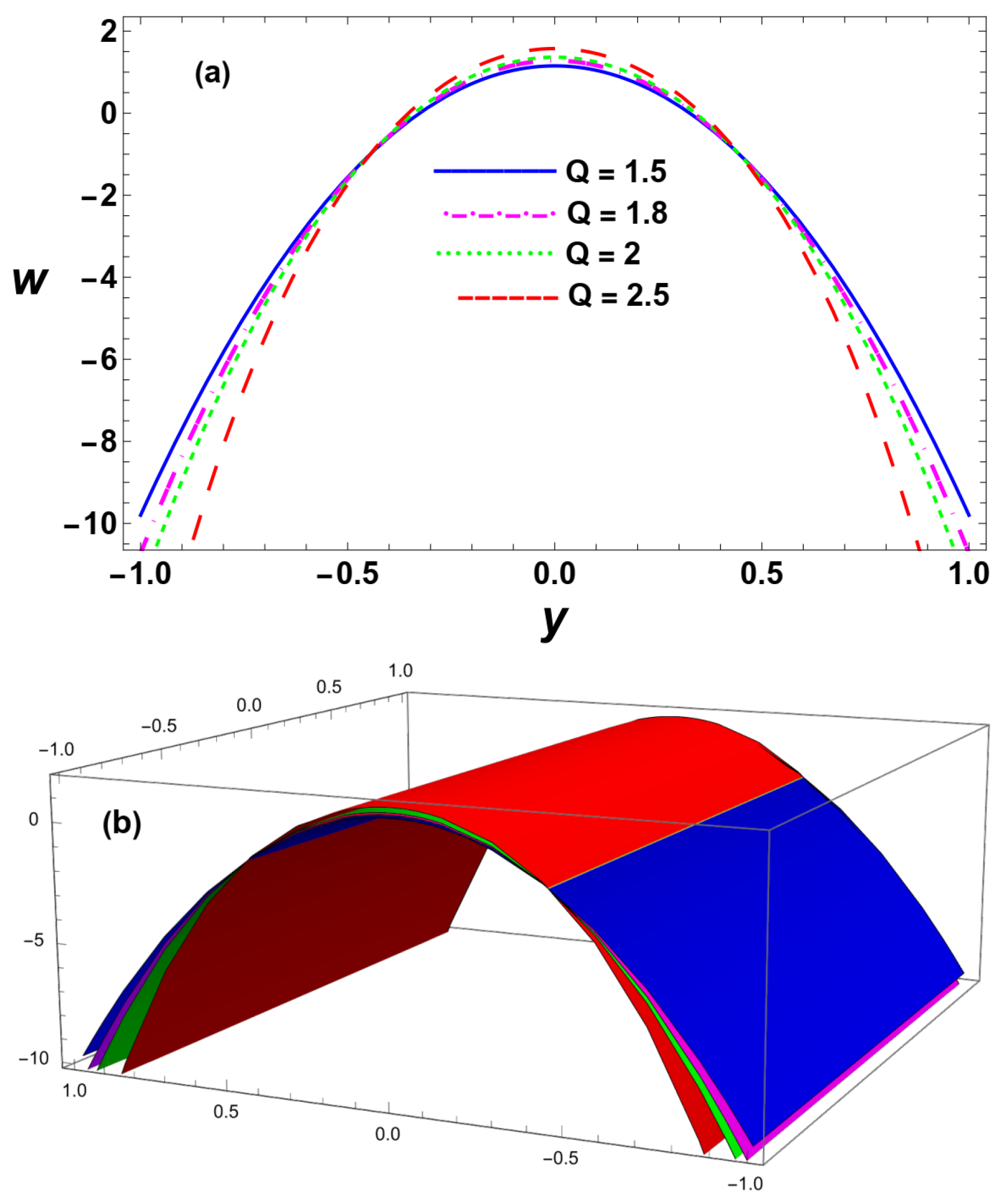
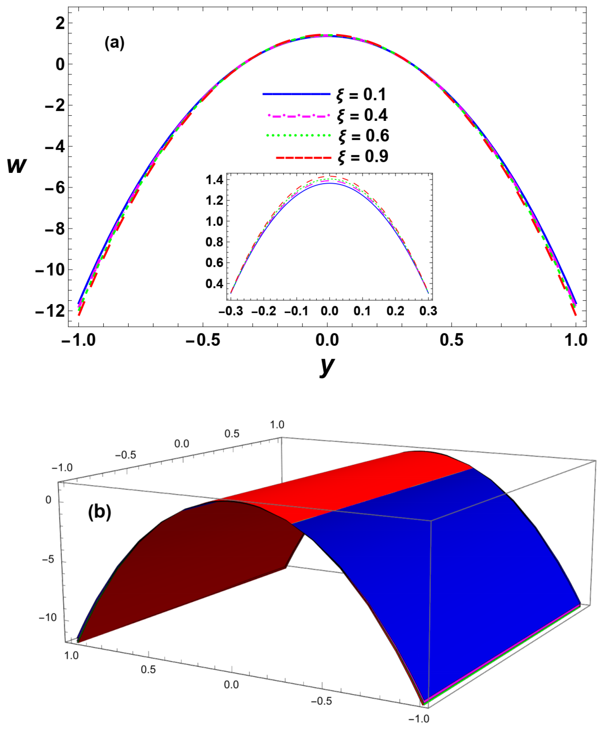
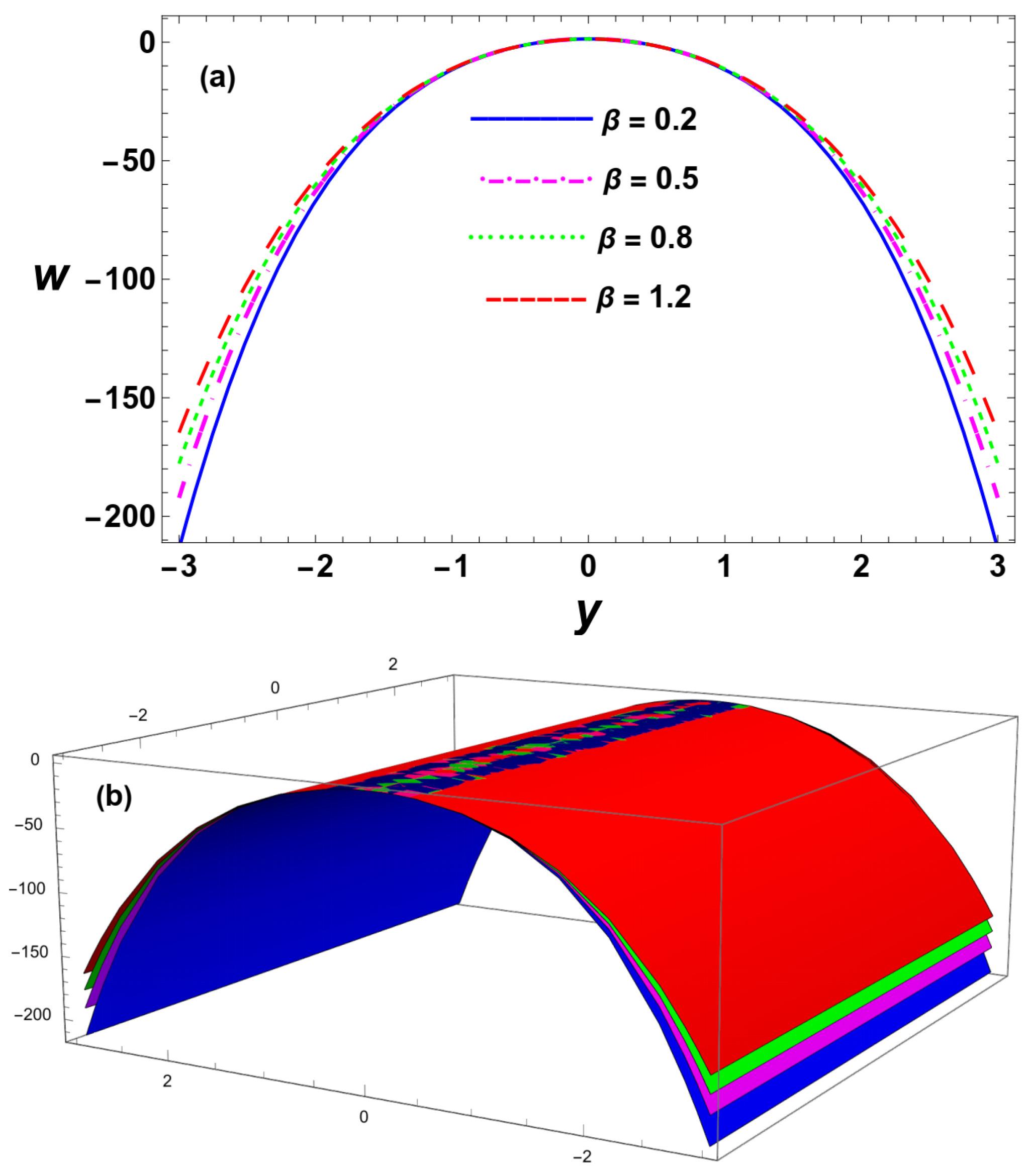
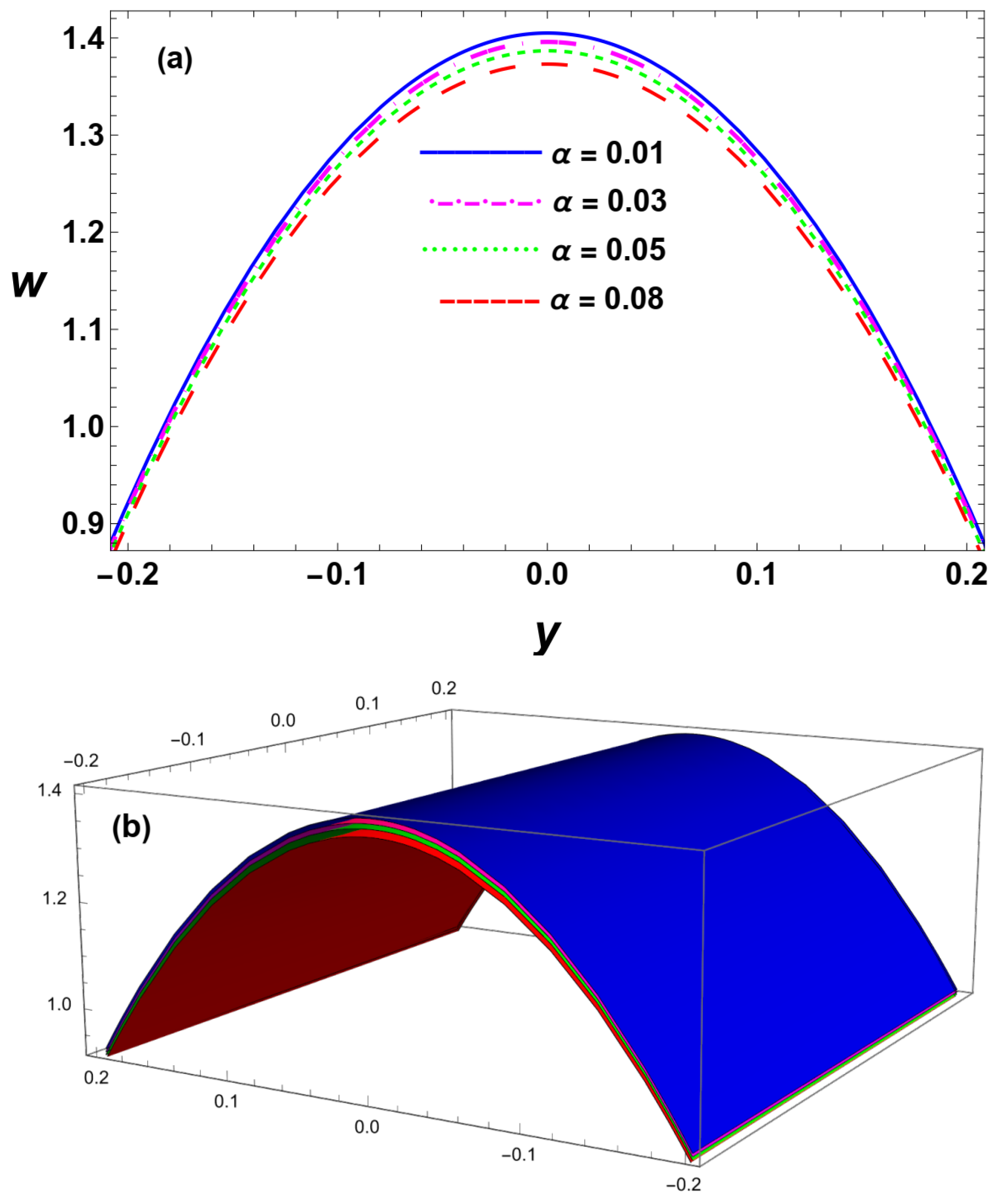
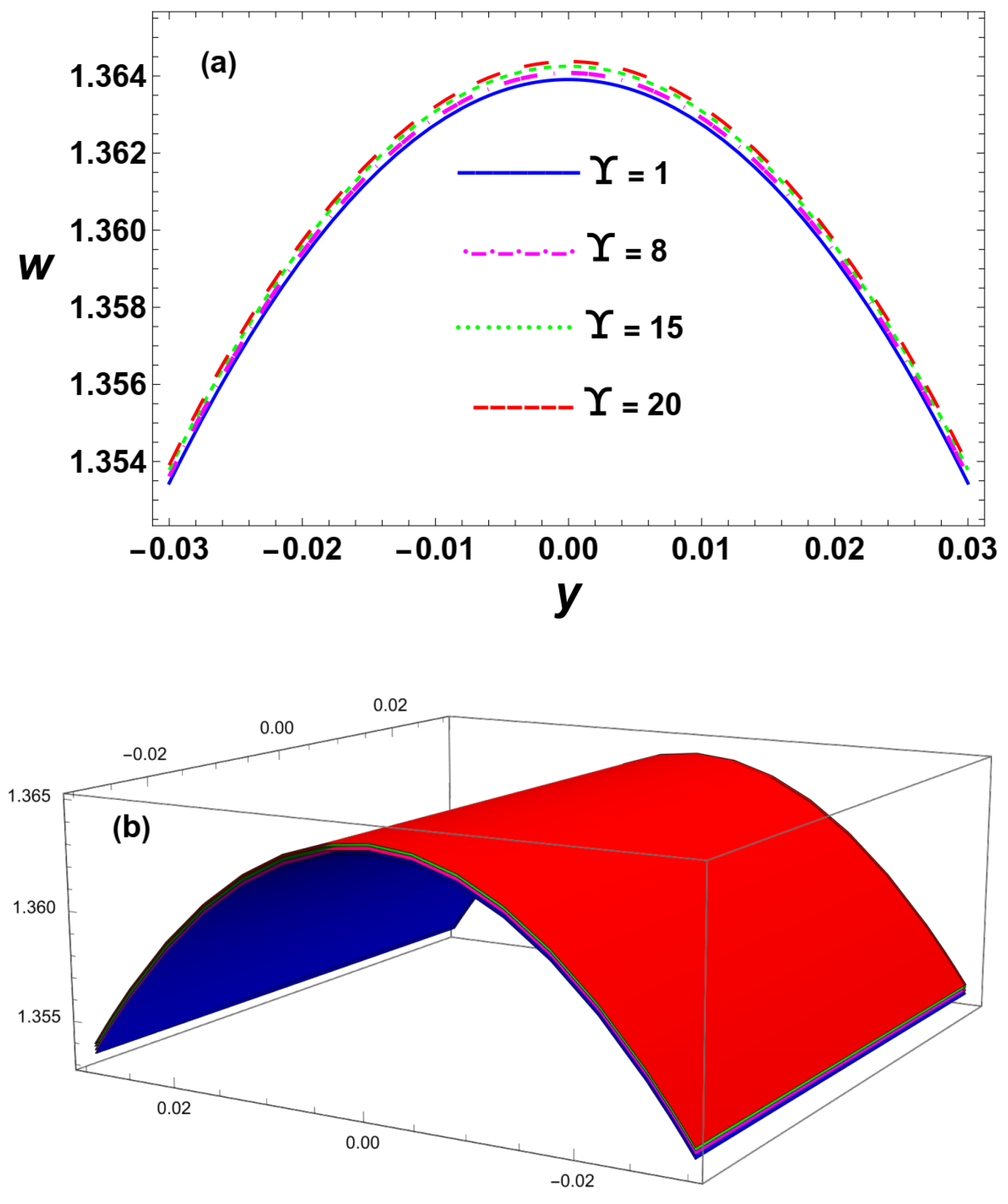
Figure 7, Figure 8, Figure 9, Figure 10 and Figure 11 provide a graph of axial velocity for the relevant parameter values. These velocity profile graphs exhibit a parabolic flow form because the fluid’s velocity is greatest in the duct’s center and diminishes as it approaches the ciliated edges. As the flow rate Q grows along the elliptic channel y-axis, Figure 7a,b demonstrate that the velocity increases in the center but in the opposite direction on both ciliated sides. Figure 8a,b graphically display velocity plotted against the wave number for metachronal wave $\xi$. The axial velocity in the middle of the elliptic duct is observed to grow as the wave number for metachronal wave values rises, and it eventually lowers as it gets closer to the ciliated duct walls. Similarly, the impacts of the cilia elliptic movement eccentricity $\epsilon$ and the thermal Grashof number ${\sigma }_T$ on the velocity profile are found to behave in the same manner as the effect of the parameter $\xi$, but figures are excluded to save space. The influence of the fluid parameter $\beta$ on flow velocity in 2D and 3D is shown in Figure 9a and Figure 9b, respectively. As the fluid parameter $\beta$ grows, the flow velocity rises on both ciliated sides and slightly converges at the duct’s center. It is observed that when parameter $\beta$ approaches zero, the fluid’s mechanics transitions from non-Newtonian (Eyring–Powell) to Newtonian. In this vertical elliptic duct, the non-Newtonian Eyring–Powell fluid will flow faster than the Newtonian fluid because the flow rate is eventually limited by decreasing values of $\beta$. Figure 10a and Figure 10b illustrate the effect of fluid parameter $\alpha$ on the velocity field in 2D and 3D, respectively. When the values of parameter $\alpha$ increase, the velocity distribution decreases along the y-axis. Similar to the previous figure, the effects of both Soret and Schmidt numbers on the velocity profile are found to behave in an identical way; however, figures are omitted to save space. This action is caused by a rise in kinematic viscosity, which raises the value of $Sc$ since the Schmidt number $Sc$ is directly proportional to kinematic viscosity. However, the mass diffusivity also drops, which eventually reduces the flow. Furthermore, the effect of the heat source parameter $\mathrm{{\rm Y}}$ is found to be in opposition to the effect of the fluid parameter $\alpha$, as seen in Figure 11a and Figure 11b, corresponding to 2D and 3D, respectively.

Figure 7. Variation in velocity profile w given by Equation (62), with y for various values of Q. (a) Two-dimensional profile; (b) Three-dimensional profile, if fixed parameters, $\alpha =0.1$, $\beta =0.2$, $ϵ=0.1$, $\mathrm{{\rm Y}}=2$, $\varphi =0.4$, ${\sigma }_T=0.2$, ${\sigma }_C=3$, $Sr=0.3$, $Sc=0.2$, $x=0.01$, $z=0.2$, $\xi =0.1$, $\epsilon =0.1$, when $Q=1.5$, $1.8$, 2, and $2.5$, respectively.

Figure 7. Variation in velocity profile w given by Equation (62), with y for various values of Q. (a) Two-dimensional profile; (b) Three-dimensional profile, if fixed parameters, $\alpha =0.1$, $\beta =0.2$, $ϵ=0.1$, $\mathrm{{\rm Y}}=2$, $\varphi =0.4$, ${\sigma }_T=0.2$, ${\sigma }_C=3$, $Sr=0.3$, $Sc=0.2$, $x=0.01$, $z=0.2$, $\xi =0.1$, $\epsilon =0.1$, when $Q=1.5$, $1.8$, 2, and $2.5$, respectively.

Figure 8. Variation in velocity profile w given by Equation (62), with y for different values of $\xi$. (a) Two-dimensional profile; (b) Three-dimensional profile, if fixed parameters, $Q=2$, $\beta =0.2$, $ϵ=0.1$, $\mathrm{{\rm Y}}=2$, $\varphi =0.4$, ${\sigma }_T=0.2$, ${\sigma }_C=3$, $Sr=0.3$, $Sc=0.2$, $x=0.01$, $z=0.2$, $\epsilon =0.1$, when $\xi =0.1$, $0.4$, $0.6$, and $0.9$, respectively.

Figure 8. Variation in velocity profile w given by Equation (62), with y for different values of $\xi$. (a) Two-dimensional profile; (b) Three-dimensional profile, if fixed parameters, $Q=2$, $\beta =0.2$, $ϵ=0.1$, $\mathrm{{\rm Y}}=2$, $\varphi =0.4$, ${\sigma }_T=0.2$, ${\sigma }_C=3$, $Sr=0.3$, $Sc=0.2$, $x=0.01$, $z=0.2$, $\epsilon =0.1$, when $\xi =0.1$, $0.4$, $0.6$, and $0.9$, respectively.

Figure 9. Variation in velocity profile w given by Equation (62), with y for different values of $\beta$. (a) Two-dimensional profile; (b) Three-dimensional profile, if fixed parameters, $Q=2$, $ϵ=0.1$, $\varphi =0.4$, $\mathrm{{\rm Y}}=2$, ${\sigma }_T=0.2$, ${\sigma }_C=3$, $Sr=0.3$, $Sc=0.2$, $\alpha =0.1$, $x=0.01$, $z=0.2$, $\epsilon =0.1$, $\xi =0.1$, when $\beta =0.2$, $0.5$, $0.8$, and $1.2$, respectively.

Figure 9. Variation in velocity profile w given by Equation (62), with y for different values of $\beta$. (a) Two-dimensional profile; (b) Three-dimensional profile, if fixed parameters, $Q=2$, $ϵ=0.1$, $\varphi =0.4$, $\mathrm{{\rm Y}}=2$, ${\sigma }_T=0.2$, ${\sigma }_C=3$, $Sr=0.3$, $Sc=0.2$, $\alpha =0.1$, $x=0.01$, $z=0.2$, $\epsilon =0.1$, $\xi =0.1$, when $\beta =0.2$, $0.5$, $0.8$, and $1.2$, respectively.

Figure 10. Variation in velocity profile w given by Equation (62), with y for different values of $\alpha$. (a) Two-dimensional profile; (b) Three-dimensional profile, if fixed parameters, $Q=2$, $\beta =0.2$, $ϵ=0.1$, $\mathrm{{\rm Y}}=2$, $\varphi =0.4$, ${\sigma }_T=0.2$, ${\sigma }_C=3$, $Sr=0.3$, $Sc=0.2$, $x=0.01$, $z=0.2$, $\epsilon =0.1$, $\xi =0.1$, when $\alpha =0.01$, $0.03$, $0.05$, and $0.08$, respectively.

Figure 10. Variation in velocity profile w given by Equation (62), with y for different values of $\alpha$. (a) Two-dimensional profile; (b) Three-dimensional profile, if fixed parameters, $Q=2$, $\beta =0.2$, $ϵ=0.1$, $\mathrm{{\rm Y}}=2$, $\varphi =0.4$, ${\sigma }_T=0.2$, ${\sigma }_C=3$, $Sr=0.3$, $Sc=0.2$, $x=0.01$, $z=0.2$, $\epsilon =0.1$, $\xi =0.1$, when $\alpha =0.01$, $0.03$, $0.05$, and $0.08$, respectively.

Figure 11. Variation in velocity profile w given by Equation (62), with y for various values of $\mathrm{{\rm Y}}$. (a) Two-dimensional profile; (b) Three-dimensional profile, if fixed parameters, $\beta =0.2$, $ϵ=0.1$, $\varphi =0.4$, $Q=2$, ${\sigma }_T=0.2$, ${\sigma }_C=3$, $\alpha =0.1$, $Sr=0.3$, $Sc=0.2$, $x=0.01$, $z=0.2$, $\epsilon =0.1$, $\xi =0.1$, when $\mathrm{{\rm Y}}=1$, 8, 15, and 20, respectively.

Figure 11. Variation in velocity profile w given by Equation (62), with y for various values of $\mathrm{{\rm Y}}$. (a) Two-dimensional profile; (b) Three-dimensional profile, if fixed parameters, $\beta =0.2$, $ϵ=0.1$, $\varphi =0.4$, $Q=2$, ${\sigma }_T=0.2$, ${\sigma }_C=3$, $\alpha =0.1$, $Sr=0.3$, $Sc=0.2$, $x=0.01$, $z=0.2$, $\epsilon =0.1$, $\xi =0.1$, when $\mathrm{{\rm Y}}=1$, 8, 15, and 20, respectively.

5.3. Pressure Gradient and Pressure Rise Profiles

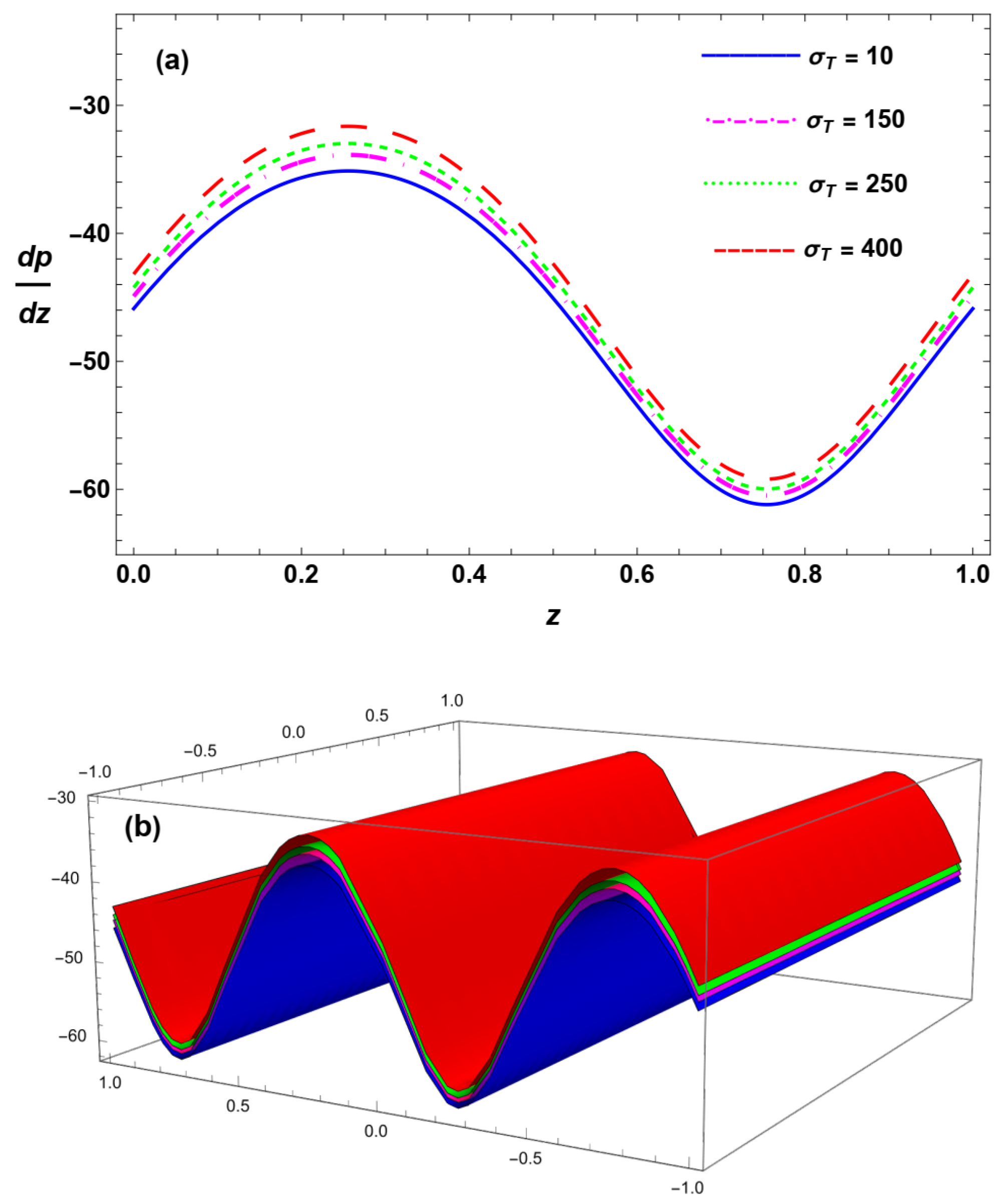
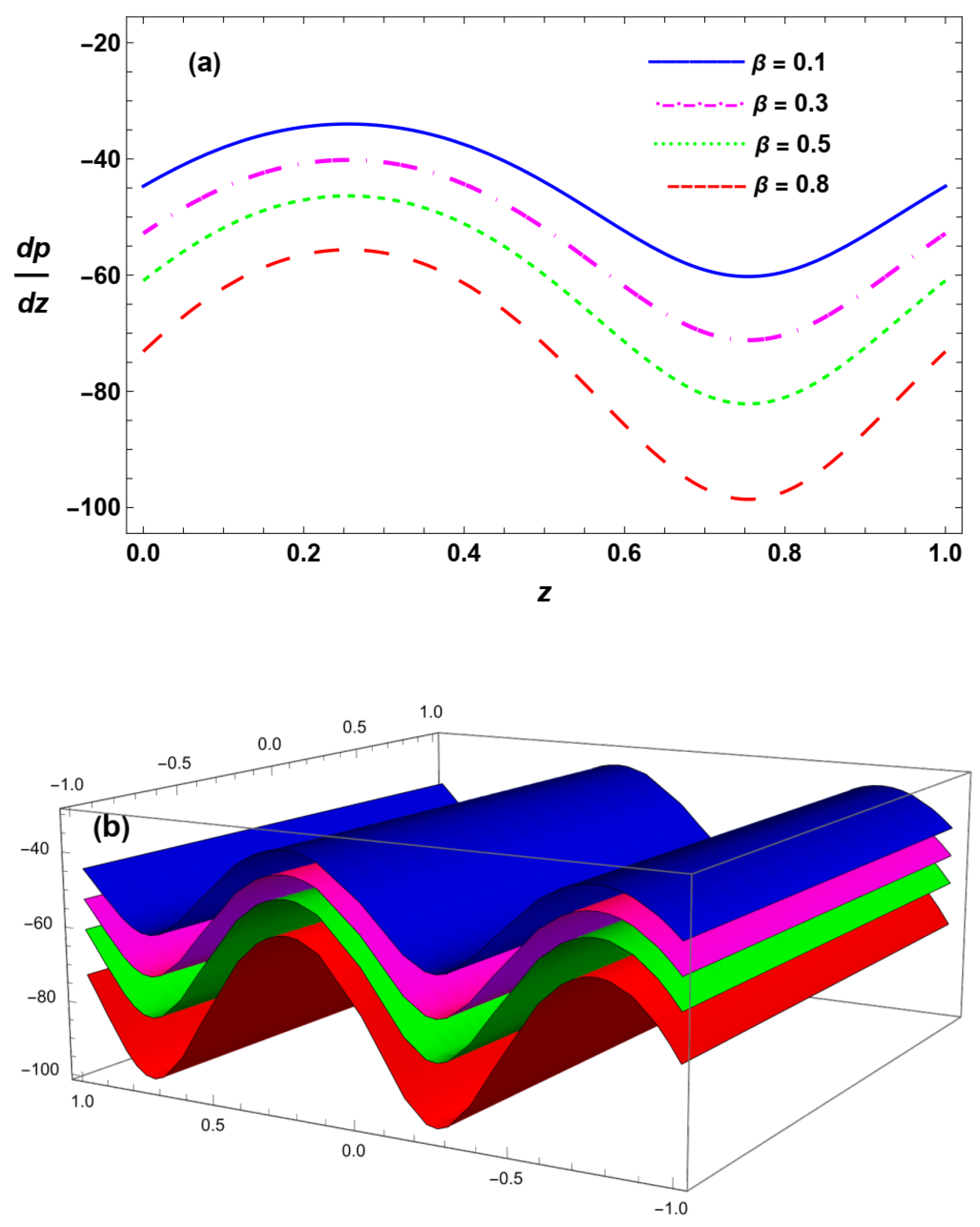
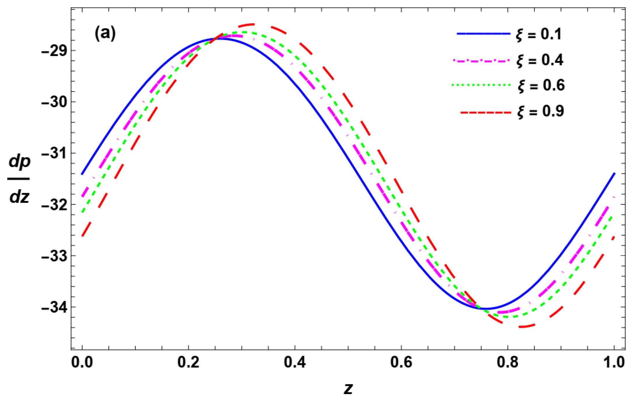
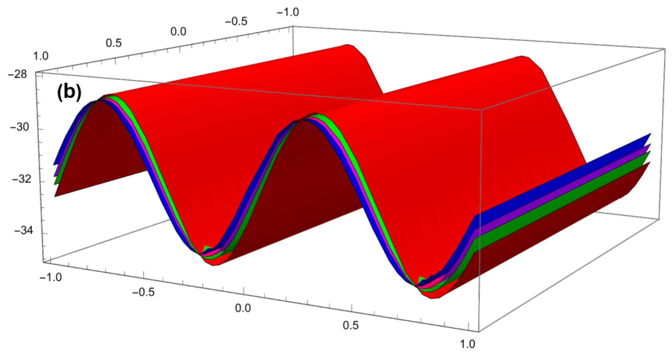
Figure 12, Figure 13 and Figure 14 illustrate the dynamics of the pressure gradient $dp/dz$ versus the z-axis for a range of physical parameters, which are included in this study. As the fluid parameter $\beta$ increases, the value of $dp/dz$ decreases, as shown in Figure 12a and Figure 12b for 2D and 3D, respectively. Similarly, it is discovered that the effects of the flow rate Q, the concentration Grashof number ${\sigma }_C$, the Soret number $Sr$, and the Schmidt number $Sc$ on the pressure gradient have the same effect to the effect of the fluid constant $\beta$ shown in Figure 12, but the corresponding figures are not provided here. As seen in Figure 13a,b, the value of $dp/dz$ declines in the first, then it enhances as the value of the wave number for metachronal wave $\xi$ rises, and then it repeats in the same manner. According to Figure 14a,b, greater values of the thermal Grashof number ${\sigma }_T$ in 2D and 3D, respectively, intensify the $dp/dz$ profile, which has the reverse trend of $\beta$, Q, $Sr$, $Sc$, and ${\sigma }_C$ on $dp/dz$.

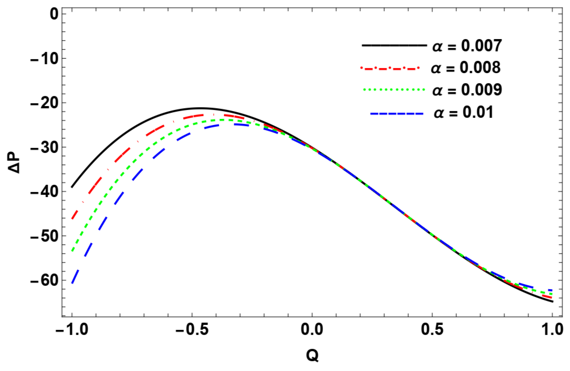
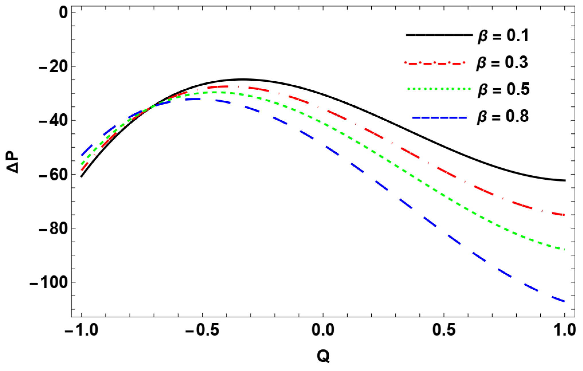
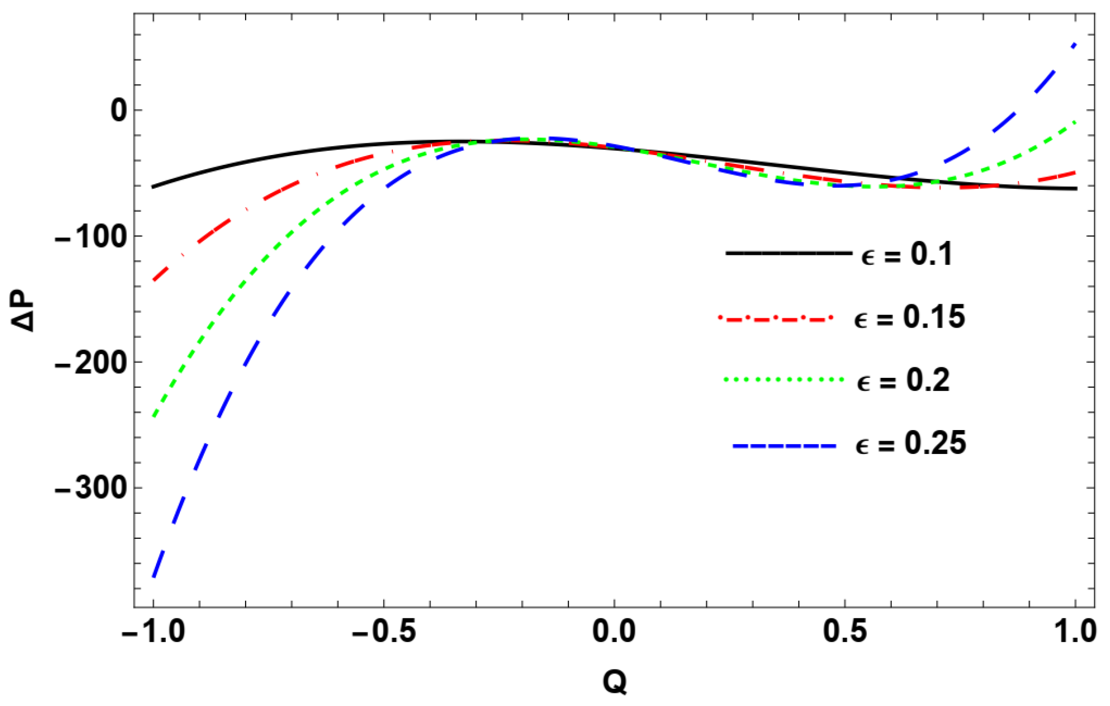
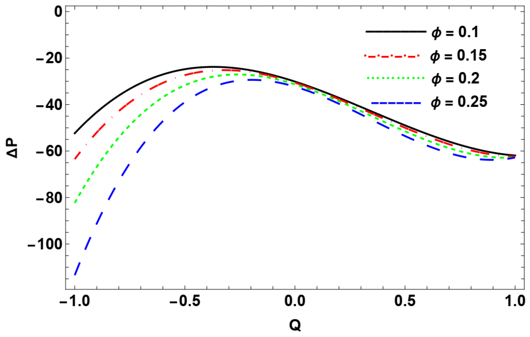
The pressure rise $\mathsf{\Delta }P$ plot versus Q for parameters $\alpha$, $\beta$, $ϵ$, and $\varphi$ is shown in Figure 15, Figure 16, Figure 17 and Figure 18, respectively. The dynamics of $\mathsf{\Delta }P$ for various values of the fluid parameter $\alpha$ are presented in Figure 15. As the fluid parameter $\alpha$ increases, the pressure rise reduces in the first, then it slightly rises. Figure 16 shows the variation in pressure rise with the flow rate Q for different values of the Eyring–Powell fluid parameter $\beta$. It is seen from this figure that the pressure rise increases for small values of flow rate, and then it decreases afterwards by increasing the values of parameter $\beta$. Figure 17 shows the graphical outcome of $\mathsf{\Delta }P$ with higher levels of aspect ratio $ϵ$. It is evident that $\mathsf{\Delta }P$ decreases initially and subsequently increases with increasing values of parameter $ϵ$. The graphical result of $\mathsf{\Delta }P$ with larger occlusion $\varphi$ values is illustrated in Figure 18. Rising values of $\varphi$ cause $\mathsf{\Delta }P$ to decrease, then slightly converge.

Figure 12. Variation in pressure gradient $dp/dz$ given by Equation (63), with z for different values of $\beta$. (a) Two-dimensional profile; (b) Three-dimensional profile, if, $ϵ=0.1$, $Q=1.2$, ${\sigma }_T=2$, ${\sigma }_C=0.1$, $Sr=0.1$, $Sc=0.2$, $\mathrm{{\rm Y}}=0.2$, $\varphi =0.14$, $\alpha =0.01$, $\xi =0.1$, $\epsilon =0.1$, when $\beta =0.1$, $0.3$, $0.5$, and $0.8$, respectively.

Figure 12. Variation in pressure gradient $dp/dz$ given by Equation (63), with z for different values of $\beta$. (a) Two-dimensional profile; (b) Three-dimensional profile, if, $ϵ=0.1$, $Q=1.2$, ${\sigma }_T=2$, ${\sigma }_C=0.1$, $Sr=0.1$, $Sc=0.2$, $\mathrm{{\rm Y}}=0.2$, $\varphi =0.14$, $\alpha =0.01$, $\xi =0.1$, $\epsilon =0.1$, when $\beta =0.1$, $0.3$, $0.5$, and $0.8$, respectively.

Figure 13. Variation in pressure gradient $dp/dz$ given by Equation (63), with z for different values of $\xi$. (a) Two-dimensional profile; (b) Three-dimensional profile, if, $ϵ=0.7$, $Q=0.1$, ${\sigma }_T=0.1$, ${\sigma }_C=1$, $Sr=0.1$, $Sc=0.2$, $\mathrm{{\rm Y}}=2$, $\varphi =0.06$, $\alpha =0.01$, $\beta =0.2$, $\epsilon =0.1$, when $\xi =0.1$, $0.4$, $0.6$, and $0.9$, respectively.

Figure 13. Variation in pressure gradient $dp/dz$ given by Equation (63), with z for different values of $\xi$. (a) Two-dimensional profile; (b) Three-dimensional profile, if, $ϵ=0.7$, $Q=0.1$, ${\sigma }_T=0.1$, ${\sigma }_C=1$, $Sr=0.1$, $Sc=0.2$, $\mathrm{{\rm Y}}=2$, $\varphi =0.06$, $\alpha =0.01$, $\beta =0.2$, $\epsilon =0.1$, when $\xi =0.1$, $0.4$, $0.6$, and $0.9$, respectively.

Figure 14. Variation in pressure gradient $dp/dz$ given by Equation (63), with z for different values of ${\sigma }_T$. (a) Two-dimensional profile; (b) Three-dimensional profile, if, $ϵ=0.1$, $\beta =0.2$, $Q=1$, ${\sigma }_C=0.1$, $Sr=0.1$, $Sc=0.2$, $\mathrm{{\rm Y}}=0.2$, $\varphi =0.14$, $\alpha =0.01$, $\epsilon =0.1$, $\xi =0.1$, when ${\sigma }_T=10$, 150, 250, and 400, respectively.

Figure 14. Variation in pressure gradient $dp/dz$ given by Equation (63), with z for different values of ${\sigma }_T$. (a) Two-dimensional profile; (b) Three-dimensional profile, if, $ϵ=0.1$, $\beta =0.2$, $Q=1$, ${\sigma }_C=0.1$, $Sr=0.1$, $Sc=0.2$, $\mathrm{{\rm Y}}=0.2$, $\varphi =0.14$, $\alpha =0.01$, $\epsilon =0.1$, $\xi =0.1$, when ${\sigma }_T=10$, 150, 250, and 400, respectively.

Figure 15. Variation in pressure rise $\mathsf{\Delta }P$ with Q for different values of $\alpha$, if, $ϵ=0.1$, $\varphi =0.14$, $\mathrm{{\rm Y}}=0.2$, $Sc=0.2$, $Sr=0.1$, ${\sigma }_C=0.1$, ${\sigma }_T=2$, $\beta =0.1$, $\epsilon =0.1$, $\xi =0.1$, when $\alpha =0.007$, $0.008$, $0.009$, and $0.01$, respectively.

Figure 15. Variation in pressure rise $\mathsf{\Delta }P$ with Q for different values of $\alpha$, if, $ϵ=0.1$, $\varphi =0.14$, $\mathrm{{\rm Y}}=0.2$, $Sc=0.2$, $Sr=0.1$, ${\sigma }_C=0.1$, ${\sigma }_T=2$, $\beta =0.1$, $\epsilon =0.1$, $\xi =0.1$, when $\alpha =0.007$, $0.008$, $0.009$, and $0.01$, respectively.

Figure 16. Variation in pressure rise $\mathsf{\Delta }P$ with Q for different values of $\beta$, if, $ϵ=0.1$, $\varphi =0.14$, $\mathrm{{\rm Y}}=0.2$, $Sc=0.2$, $Sr=0.1$, ${\sigma }_C=0.1$, ${\sigma }_T=2$, $\alpha =0.01$, $\epsilon =0.1$, $\xi =0.1$, when $\beta =0.1$, $0.3$, $0.5$, and $0.8$, respectively.

Figure 16. Variation in pressure rise $\mathsf{\Delta }P$ with Q for different values of $\beta$, if, $ϵ=0.1$, $\varphi =0.14$, $\mathrm{{\rm Y}}=0.2$, $Sc=0.2$, $Sr=0.1$, ${\sigma }_C=0.1$, ${\sigma }_T=2$, $\alpha =0.01$, $\epsilon =0.1$, $\xi =0.1$, when $\beta =0.1$, $0.3$, $0.5$, and $0.8$, respectively.

Figure 17. Variation in pressure rise $\mathsf{\Delta }P$ with Q for different values of $ϵ$, if, $\beta =0.1$, $\varphi =0.14$, $\mathrm{{\rm Y}}=0.2$, $Sc=0.2$, $Sr=0.1$, ${\sigma }_C=0.1$, ${\sigma }_T=2$, $\alpha =0.01$, $\epsilon =0.1$, $\xi =0.1$, when $ϵ=0.1$, $0.15$, $0.2$, and $0.25$, respectively.

Figure 17. Variation in pressure rise $\mathsf{\Delta }P$ with Q for different values of $ϵ$, if, $\beta =0.1$, $\varphi =0.14$, $\mathrm{{\rm Y}}=0.2$, $Sc=0.2$, $Sr=0.1$, ${\sigma }_C=0.1$, ${\sigma }_T=2$, $\alpha =0.01$, $\epsilon =0.1$, $\xi =0.1$, when $ϵ=0.1$, $0.15$, $0.2$, and $0.25$, respectively.

Figure 18. Variation in pressure rise $\mathsf{\Delta }P$ with Q for different values of $\varphi$, if, $ϵ=0.1$, $\beta =0.1$, $\mathrm{{\rm Y}}=0.2$, $Sc=0.2$, $Sr=0.1$, ${\sigma }_C=0.1$, ${\sigma }_T=2$, $\alpha =0.01$, $\epsilon =0.1$, $\xi =0.1$, when $\varphi =0.1$, $0.15$, $0.2$, and $0.25$, respectively.

Figure 18. Variation in pressure rise $\mathsf{\Delta }P$ with Q for different values of $\varphi$, if, $ϵ=0.1$, $\beta =0.1$, $\mathrm{{\rm Y}}=0.2$, $Sc=0.2$, $Sr=0.1$, ${\sigma }_C=0.1$, ${\sigma }_T=2$, $\alpha =0.01$, $\epsilon =0.1$, $\xi =0.1$, when $\varphi =0.1$, $0.15$, $0.2$, and $0.25$, respectively.

5.4. Streamline Pattern

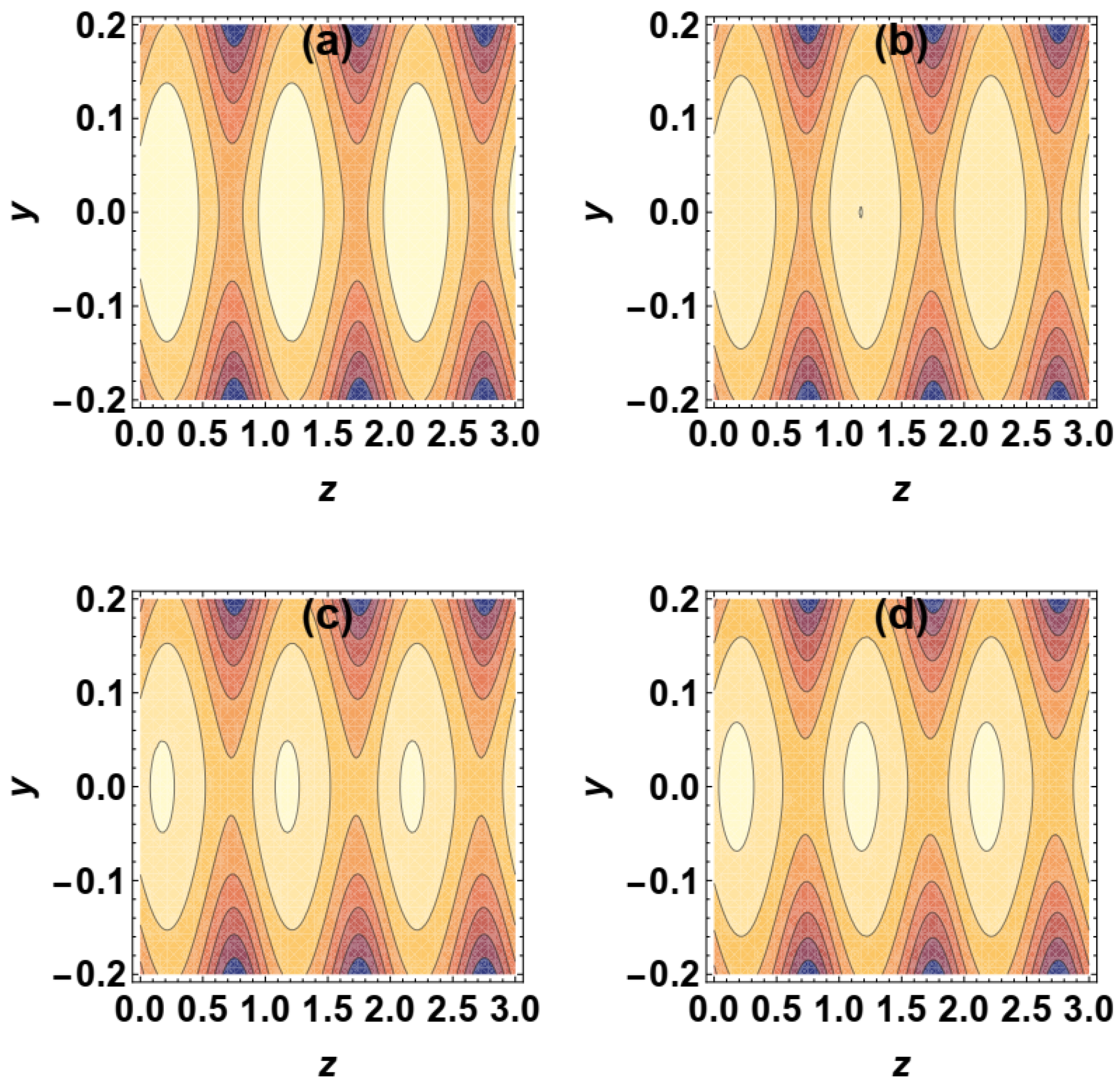
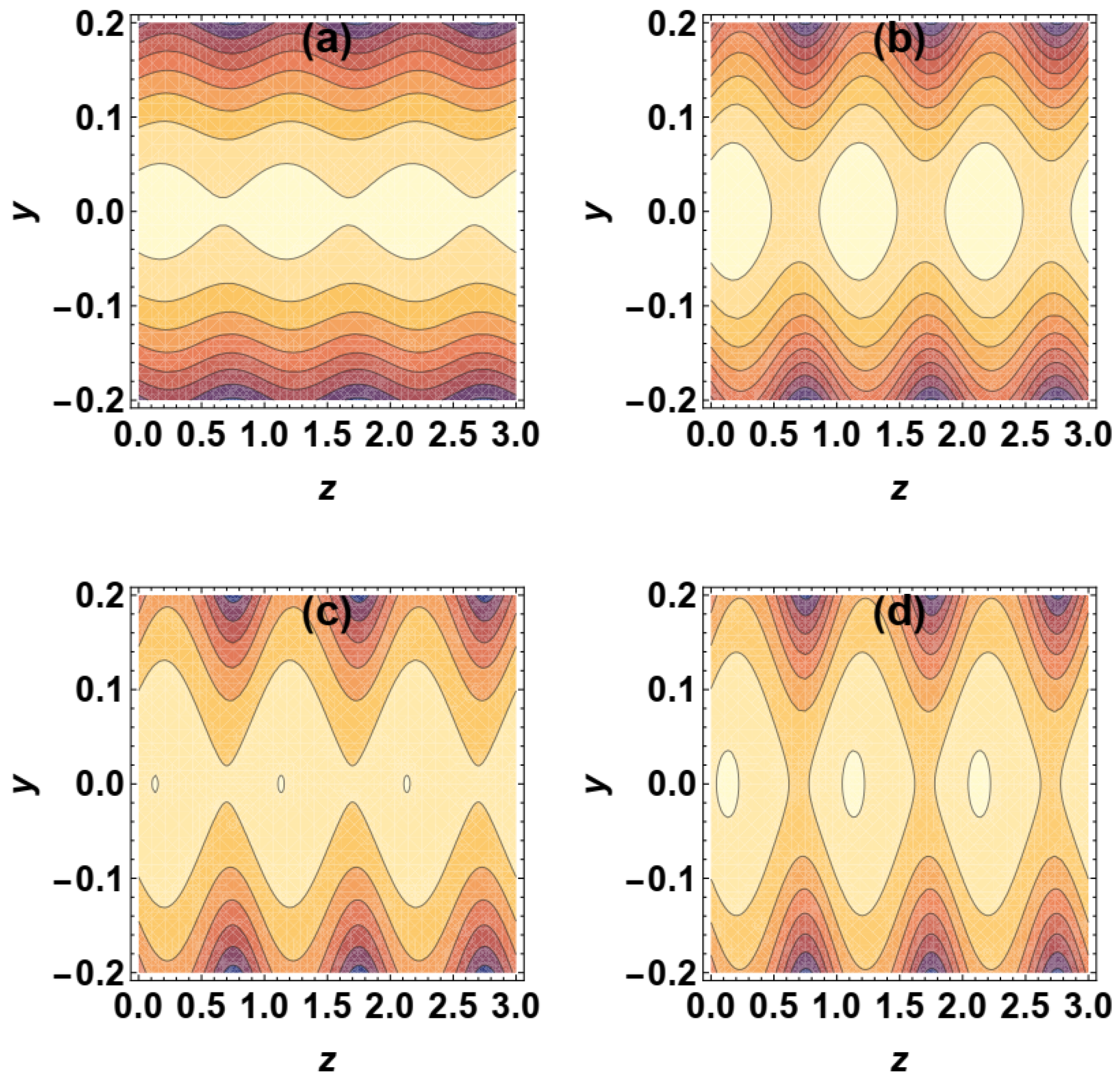
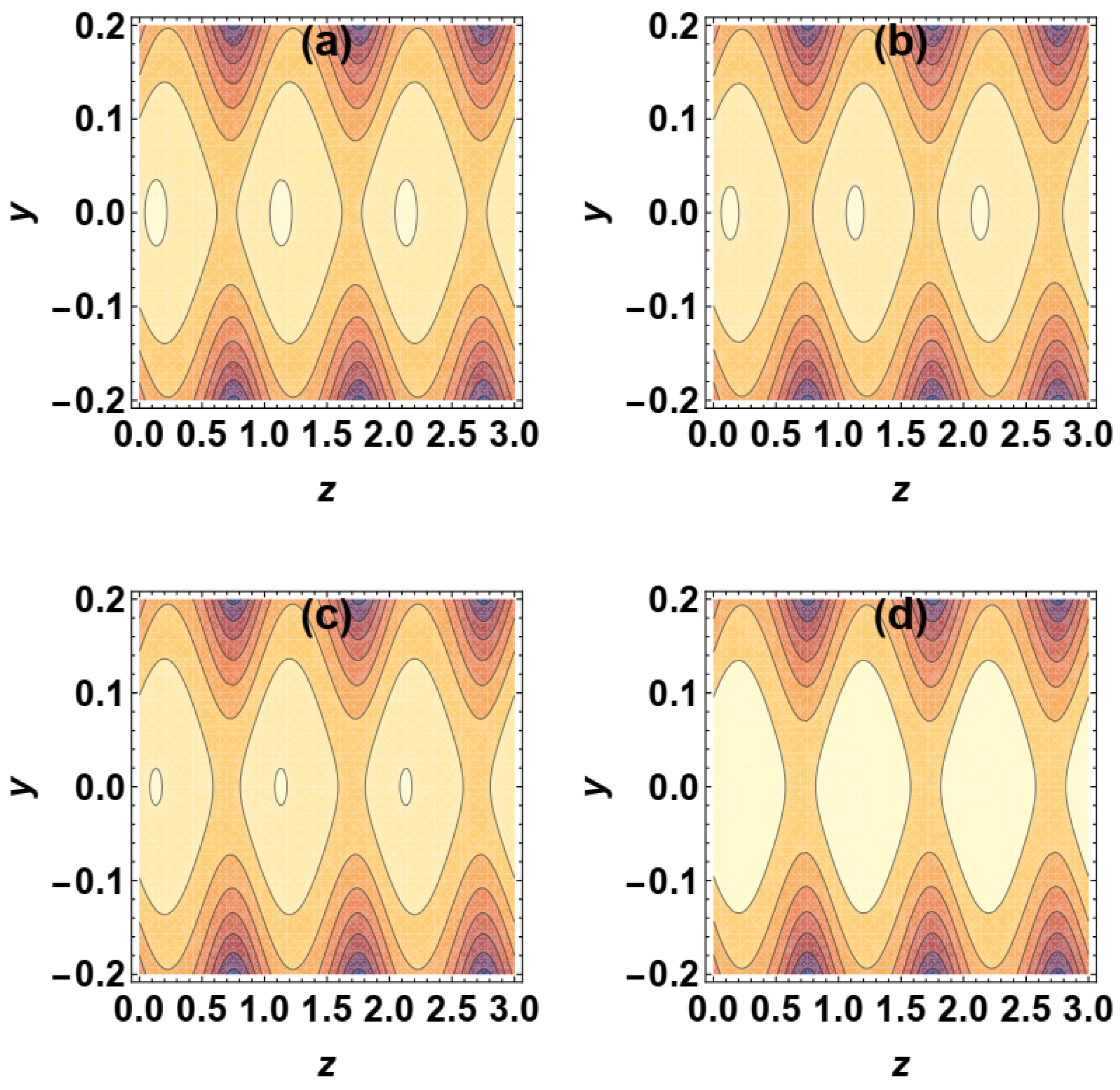
The impact of various parameters on flow pattern in this ciliated elliptic duct appears graphically by the streamlines shown in Figure 19, Figure 20 and Figure 21. The way streamlines react to rising volumetric flow rate values is seen in Figure 19a–d. As the volumetric flow rate Q rises, it is seen that the trapping bolus’s size grows in tandem with the number of forms. Figure 20a–d display the streamlines analysis for various values of $\varphi$. This demonstrates that as $\varphi$ grows, the number and size of contours increase. Figure 21a–d illustrate how the fluid parameter $\alpha$ affects the trapped bolus, leading to a decrease in trapping size with enhancing the parameter $\alpha$.

6. Concluding Remarks

Investigating the peristaltic flow of heated Eyring–Powell fluid in a conduit with ciliated walls and an elliptic cross-section under the mass transfer impact is the goal of this work. The main conclusions of this study are:

(1) In an elliptic duct, the concentration profile behaves differently from the velocity and temperature profiles, which rise in the center and progressively drop towards the ciliated walls.

(2) In this vertical ciliated elliptic duct, the non-Newtonian Eyring–Powell fluid will move faster than the Newtonian fluid.

(3) It is evident that the heat absorption parameter has a dual effect on the temperature profile; that is, when the heat absorption parameter values are increased, the temperature rises in the middle of the elliptic duct, while it falls close to the ciliated edges, which is the same manner on the velocity profile for parameters $\xi$, ${\sigma }_T$, Q, and $\epsilon$.

(4) With increasing levels of the heat absorption parameter, Soret, and Schmidt numbers, the concentration rises along the ciliated duct walls and falls in the center of the duct.

(5) Fluid velocity clearly decreases as all of the fluid parameter $\alpha$, concentration Grashof number, Soret number, and Schmidt number improve down the axis, but it exhibits the opposite behavior for greater heat absorption parameter values.

(6) The pressure gradient is directly affected by the thermal Grashof number, but it is inversely affected by the flow velocity, fluid parameter $\beta$, solutal Grashof number, and Soret number.

(7) It is discovered that the fluid parameter $\alpha$ and the aspect ratio $ϵ$ both reduce the pressure rise initially before increasing it later, whereas the fluid parameter $\beta$ has the opposite effect.

(8) The trapping of streamlines increases in size with increasing values of flow rate and occlusion, but the opposite dynamic is true for the fluid parameter $\alpha$.

References

1. Lardner, T.J.; Shack, W.J. Cilia transport. Bull. Math. Biophys. 1972, 34, 325–335. [Google Scholar] [CrossRef] [Scilit]
2. Blake, J. Flow in tubules due to ciliary activity. Bull. Math. Biol. 1973, 35, 513–523. [Google Scholar] [CrossRef] [Scilit]
3. Akbar, N.S.; Khan, Z.H. Heat transfer study of an individual multiwalled carbon nanotube due to metachronal beating of cilia. Int. Commun. Heat Mass Transf. 2014, 59, 114–119. [Google Scholar] [CrossRef] [Scilit]
4. Akbar, N.S.; Butt, A.W. Heat transfer analysis of viscoelastic fluid flow due to metachronal wave of cilia. Int. J. Biomath. 2014, 7, 1450066. [Google Scholar] [CrossRef] [Scilit]
5. Sher Akbar, N. Biomathematical analysis of carbon nanotubes due to ciliary motion. Int. J. Biomath. 2015, 8, 1550023. [Google Scholar] [CrossRef] [Scilit]
6. Butt, A.W.; Akbar, N.S.; Mir, N.A. Heat transfer analysis of peristaltic flow of a Phan-Thien–Tanner fluid model due to metachronal wave of cilia. Biomech. Model. Mechanobiol. 2020, 19, 1925–1933. [Google Scholar] [CrossRef] [Scilit] [PubMed]
7. Saleem, A.; Akhtar, S.; Alharbi, F.M.; Nadeem, S.; Ghalambaz, M.; Issakhov, A. Physical aspects of peristaltic flow of hybrid nano fluid inside a curved tube having ciliated wall. Results Phys. 2020, 19, 103431. [Google Scholar] [CrossRef] [Scilit]
8. Kada, B.; Pasha, A.A.; Asghar, Z.; Khan, M.W.S.; Aris, I.B.; Shaikh, M.S. Carreau–Yasuda fluid flow generated via metachronal waves of cilia in a micro-channel. Phys. Fluids 2023, 35, 013110. [Google Scholar] [CrossRef] [Scilit]
9. Imran, A.; Abbas, M.; Awan, S.E.; Shoaib, M.; Raja, M.A. Electro osmotic flow of nanofluids within a porous symmetric tapered ciliated channel. ZAMM—J. Appl. Math. Mech. /Z. Angew. Math. Mech. 2024, 104, e202300838. [Google Scholar] [CrossRef] [Scilit]
10. Abbasi, A.; Danish, S.; Farooq, W.; Khan, M.I.; Akermi, M.; Hejazi, A.H. Peristaltic transport of viscoelastic fluid in curved ducts with ciliated walls. Phys. Fluids 2024, 36, 033619. [Google Scholar] [CrossRef] [Scilit]
11. Hafez, N.M.; Abd-Alla, A.M.; Metwaly, T.M.N. Influences of rotation and mass and heat transfer on MHD peristaltic transport of Casson fluid through inclined plane. Alex. Eng. J. 2023, 68, 665–692. [Google Scholar] [CrossRef] [Scilit]
12. Hafez, N.M.; Abd-Alla, A.M.; Mahmoud, S.R. A thermo-magnetohydrodynamic particle-fluid suspension moves peristaltically through a porous medium. Alex. Eng. J. 2025, 112, 598–632. [Google Scholar] [CrossRef] [Scilit]
13. Alkharashi, S.A.; Assaf, A. Thermodynamics of a Liquid Film in the Presence of External Shear Stress. J. Appl. Fluid Mech. 2020, 13, 753–766. [Google Scholar] [CrossRef] [Scilit]
14. Sirwah, M.; Alkharashi, S.A. Dynamic Modeling of Heated Oscillatory Layer of non-Newtonian Liquid. Fluid Dyn. 2021, 56, 291–307. [Google Scholar] [CrossRef] [Scilit]
15. Alkharashi, S.A.; Sirwah, M. Dynamical Responses of Inclined Heated channel of MHD Dusty Fluids Through Porous Media. J. Eng. Math. 2021, 130, 5. [Google Scholar] [CrossRef] [Scilit]
16. Hafez, N.M.; Alsemiry, R.D.; Abd-Alla, S.A.; Abd-Alla, A.M. Peristaltic transport characteristics of a second-grade dusty fluid flown with heat transfer through a tube revisited. Sci. Rep. 2022, 12, 21605. [Google Scholar] [CrossRef] [Scilit]
17. Hafez, N.M. EHD peristaltic flow of Sisko fluid under the effects of convection and endoscope. Ain Shams Eng. J. 2024, 15, 102647. [Google Scholar] [CrossRef] [Scilit]
18. Huang, Y.M.; Ho, C.H. Study of the Fluid Flow in the Elliptical Duct by the Method of Characteristics. ASME J. Press. Vessel Technol. 1993, 115, 80–84. [Google Scholar] [CrossRef] [Scilit]
19. Saleem, A.; Akhtar, S.; Nadeem, S.; Alharbi, F.M.; Ghalambaz, M.; Issakhov, A. Mathematical computations for Peristaltic flow of heated non-Newtonian fluid inside a sinusoidal elliptic duct. Phys. Scr. 2020, 95, 105009. [Google Scholar] [CrossRef] [Scilit]
20. Nadeem, S.; Akhtar, S.; Saleem, A. Peristaltic flow of a heated Jeffrey fluid inside an elliptic duct: Streamline analysis. Appl. Math. Mech. 2021, 42, 583–592. [Google Scholar] [CrossRef] [Scilit]
21. Akhtar, S.; McCash, L.B.; Nadeem, S.; Saleem, S.; Issakhov, A. Convective heat transfer for Peristaltic flow of SWCNT inside a sinusoidal elliptic duct. Sci. Prog. 2021, 104, 00368504211023683. [Google Scholar] [CrossRef] [Scilit]
22. Rachid, H.; Ouazzani, M.; Lahlou, N. Entropy generation and mechanical efficiency in laminar peristaltic flow through an elliptical duct. Heat Transf. 2021, 50, 8525–8539. [Google Scholar] [CrossRef] [Scilit]
23. McCash, L.B.; Akhtar, S.; Nadeem, S.; Saleem, S. Entropy analysis of the peristaltic flow of hybrid nanofluid inside an elliptic duct with sinusoidally advancing boundaries. Entropy 2021, 23, 732. [Google Scholar] [CrossRef] [Scilit]
24. Devaki, P. Peristaltic Effects on Flow of Hybrid Nanofluid in an Elliptic Duct with Elasticity. Commun. Math. Appl. 2022, 13, 943–953. [Google Scholar] [CrossRef] [Scilit]
25. Nadeem, S.; Haider, J.A.; Akhtar, S.; Mohamed, A. Insight into the dynamics of the Rabinowitsch fluid through an elliptic duct: Peristalsis analysis. Front. Phys. 2022, 10, 923269. [Google Scholar] [CrossRef] [Scilit]
26. Akhtar, S.; Shahzad, M.H.; Nadeem, S.; Awan, A.U.; Almutairi, S.; Ghazwani, H.A.; Sayed, M.M. Analytical solutions of PDEs by unique polynomials for peristaltic flow of heated Rabinowitsch fluid through an elliptic duct. Sci. Rep. 2022, 12, 12943. [Google Scholar] [CrossRef] [Scilit]
27. Shahzad, M.H.; Awan, A.U.; Akgül, A.; Nadeem, S.; Guedri, K.; Hassani, M.K.; Makhdoum, B.M. Analytical investigation of Carreau fluid flow through a non-circular conduit with wavy wall. Sci. Rep. 2024, 14, 2473. [Google Scholar] [CrossRef] [Scilit] [PubMed]
28. Shahzad, M.H.; Awan, A.U.; Nadeem, S.; Ahammad, N.A.; Hamam, H.; Alamer, A.; Shafique, S. Rheological effects in peristaltic flow of Prandtl fluid through elliptical duct: A comprehensive analysis. ZAMM—J. Appl. Math. Mech./Z. Angew. Math. Mech. 2024, 104, e202400094. [Google Scholar] [CrossRef] [Scilit]
29. McCash, L.B.; Nadeem, S.; Akhtar, S.; Saleem, A.; Saleem, S.; Issakhov, A. Novel idea about the peristaltic flow of heated Newtonian fluid in elliptic duct having ciliated walls. Alex. Eng. J. 2021, 61, 2697–2707. [Google Scholar] [CrossRef] [Scilit]
30. Nadeem, S.; Akhtar, S.; Almutairi, S.; Ghazwani, H.A.; Elkhatib, S.E. Physical survey of thermally heated non-newtonian jeffrey fluid in a ciliated conduit having heated compressing and expanding walls. Appl. Sci. 2022, 12, 5065. [Google Scholar] [CrossRef] [Scilit]
31. Fuzhang, W.; Akhtar, S.; Nadeem, S.; El-Shafay, A.S. Mathematical computations for the physiological flow of Casson fluid in a vertical elliptic duct with ciliated heated wavy walls. Waves Random Complex Media 2022, 35, 5919–5932. [Google Scholar] [CrossRef] [Scilit]
32. Ghazwani, H.A.; Akhtar, S.; Almutairi, S.; Saleem, A.; Nadeem, S.; Mahmoud, O. Insightful facts on peristalsis flow of water conveying multi-walled carbon nanoparticles through elliptical ducts with ciliated walls. Front. Phys. 2022, 10, 923290. [Google Scholar] [CrossRef] [Scilit]
33. Nadeem, S.; Akhtar, S.; Alharbi, F.M.; Saleem, S.; Issakhov, A. Analysis of heat and mass transfer on the peristaltic flow in a duct with sinusoidal walls: Exact solutions of coupled PDEs. Alex. Eng. J. 2022, 61, 4107–4117. [Google Scholar] [CrossRef] [Scilit]
34. Akhtar, S.; Almutairi, S.; Nadeem, S. Impact of heat and mass transfer on the Peristaltic flow of non-Newtonian Casson fluid inside an elliptic conduit: Exact solutions through novel technique. Chin. J. Phys. 2022, 78, 194–206. [Google Scholar] [CrossRef] [Scilit]
35. Nadeem, S.; Waqar, H.; Akhtar, S.; Zidan, A.M.; Almutairi, S.; Ghazwani, H.A.S.; Alaoui, M.K.; El-Waked, M.T. Mathematical assessment of convection and diffusion analysis for a non-circular duct flow with viscous dissipation: Application of physiology. Symmetry 2022, 14, 1536. [Google Scholar] [CrossRef] [Scilit]
36. Nadeem, S.; Akhtar, S.; Akkurt, N.; Saleem, A.; Almutairi, S.; Ghazwani, H.A. Physiological peristaltic flow of Jeffrey fluid inside an elliptic cross section with heat and mass transfer: Exact solutions through Polynomial solution technique. ZAMM—J. Appl. Math. Mech. /Z. Angew. Math. Mech. 2023, 103, e202100383. [Google Scholar] [CrossRef] [Scilit]
37. Akbar, N.S.; Nadeem, S. Characteristics of heating scheme and mass transfer on the peristaltic flow for an Eyring–Powell fluid in an endoscope. Int. J. Heat Mass Transf. 2012, 55, 375–383. [Google Scholar] [CrossRef] [Scilit]
38. Hayat, T.; Shah, S.I.; Ahmad, B.; Mustafa, M. Effect of slip on peristaltic flow of Powell-Eyring fluid in a symmetric channel. Appl. Bionics Biomech. 2014, 11, 69–79. [Google Scholar] [CrossRef] [Scilit]
39. Abbasi, F.M.; Alsaedi, A.; Hayat, T. Peristaltic Transport of Eyring-Powell Fluid in a Curved Channel. J. Aerosp. Eng. 2014, 27, 04014037. [Google Scholar] [CrossRef] [Scilit]
40. Hina, S.; Mustafa, M.; Hayat, T.; Alsaedi, A. Peristaltic flow of Powell-Eyring fluid in curved channel with heat transfer: A useful application in biomedicine. Comput. Methods Programs Biomed. 2016, 135, 89–100. [Google Scholar] [CrossRef] [Scilit]
41. Hina, S.; Mustafa, M.; Hayat, T.; Alsaedi, A. Peristaltic transport of Powell–Eyring fluid in a curved channel with heat/mass transfer and wall properties. Int. J. Heat Mass Transf. 2016, 101, 156–165. [Google Scholar] [CrossRef] [Scilit]
42. Awan, A.U.; Fathima, D.; Shahzad, M.H.; Alqarni, M.M.; Nadeem, S.; Hamam, H. Investigation of Erying–Powell fluid flow in the elliptical multi-stenosed artery: Application of perturbation method via polynomial solutions. ZAMM—J. Appl. Math. Mech./Z. Angew. Math. Mech. 2023, 104, e202300603. [Google Scholar] [CrossRef] [Scilit]
43. Akram, M.; Shahzad, M.H.; Ahammad, N.A.; Gamaoun, F.; Awan, A.U.; Hamam, H.; Alroobaea, R. Rheology of Eyring-Powell hybrid nanofluid flow under the peristaltic effects through an elliptical conduit: Analytical investigation. Results Phys. 2024, 59, 107602. [Google Scholar] [CrossRef] [Scilit]
44. Shahzad, M.H.; Akram, M.; Nadeem, S.; Ahammad, N.A.; Awan, A.U.; Alzubadi, H. Investigation of Prandtl-Eyring fluid flow under the influence of peristalsis through an inclined elliptic channel. Numer. Heat Transf. Part A Appl. 2024, 86, 8721–8739. [Google Scholar] [CrossRef] [Scilit]
45. Hafez, N.M.; Abd-Alla, A.M.; Bayones, F.S. Eyring-Powell fluid’s structure via an elliptic duct: Peristalsis analysis under the influence of mass and heat transmission. Case Stud. Therm. Eng. 2025, 76, 107249. [Google Scholar] [CrossRef] [Scilit]
46. Hayman, W.K.; Shanidze, Z.G. Polynomial solution of partial differential equations. Method Appl. Anal. 1999, 6, 97–108. [Google Scholar] [CrossRef] [Scilit]
Figure 1. Sketch of the profile geometry.
Dynamics 06 00014 g001
Figure 2. The motion of a cilium.
Dynamics 06 00014 g002
Figure 3. Validation of present work, (a) Comparison with results reported in [29], and (b) Comparison with results reported in [31], if; ϵ = 0.1 , Υ = 2 , Q = 2 , ϕ = 0.4 , S r = 0.3 , S c = 0.2 , x = 0.01 , z = 0.2 , ξ = 0.1 , ε = 0.1 when (a) α = β = 0 , σ T = 0.2 , σ C = 3 ; (b) σ T = 0.2 , σ C = 0 , α = 0 , β = 0.1 .
Dynamics 06 00014 g003
Figure 19. Streamline patterns for various values of Q, if, (a) Q = 0.1 , (b) Q = 0.15 , (c) Q = 0.2 , and (d) Q = 0.25 , when ϵ = 0.1 , β = 0.2 , Υ = 0.1 , S c = 0.2 , S r = 0.1 , σ C = 3 , σ T = 2 , α = 0.01 , ϕ = 0.3 , ε = 0.3 , ξ = 0.1 , and x = 0.01 .
Dynamics 06 00014 g019
Figure 20. Streamline patterns for various values of ϕ , if, (a) ϕ = 0.05 , (b) ϕ = 0.15 , (c) ϕ = 0.25 , and (d) ϕ = 0.3 , when ϵ = 0.1 , β = 0.2 , Υ = 0.1 , S c = 0.2 , S r = 0.1 , σ C = 3 , σ T = 2 , α = 0.01 , Q = 0.6 , ε = 0.3 , ξ = 0.1 , and x = 0.01 .
Dynamics 06 00014 g020
Figure 21. Streamline patterns for various values of α , if, (a) α = 0.01 , (b) α = 0.02 , (c) α = 0.03 , and (d) α = 0.04 , when ϵ = 0.1 , β = 0.2 , Υ = 0.1 , S c = 0.2 , S r = 0.1 , σ C = 3 , σ T = 2 , Q = 0.6 , ϕ = 0.3 , ε = 0.3 , ξ = 0.1 , and x = 0.01 .
Dynamics 06 00014 g021
Disclaimer/Publisher’s Note: The statements, opinions and data contained in all publications are solely those of the individual author(s) and contributor(s) and not of MDPI and/or the editor(s). MDPI and/or the editor(s) disclaim responsibility for any injury to people or property resulting from any ideas, methods, instructions or products referred to in the content.