Analytical Representation and Applications of Solutions to a Loaded Fractional Integro-Differential Equation

Abstract

We study the Cauchy problem for a loaded fractional integro-differential equation with a time-dependent diffusion coefficient. By reducing the problem to an equivalent Volterra integral equation of the second kind, we derive explicit analytical representations of solutions under appropriate regularity assumptions. The construction of the associated resolvent kernel allows us to establish existence and uniqueness results and to investigate the role of the fractional order and the loading term in the solution structure. Two illustrative examples are presented to demonstrate the applicability of the proposed approach.

1. Introduction and Formulation of the Problem

In recent decades, boundary value and Cauchy problems for heat and wave equations incorporating fractional loading terms have attracted considerable attention. Such models arise naturally in mathematical physics, continuum mechanics, and materials science, particularly in the description of processes governed by memory, hereditary effects, and anomalous diffusion phenomena.

A substantial body of research has been devoted to the analytical study of diffusion equations with fractional loading. In particular, Kosmakova et al. [1] investigated the heat equation with fractional load and derived solvability conditions within an appropriate functional framework. This line of research was further developed in [2], where boundary value problems with fractional integral loading were analyzed. The well-posedness of heat equations with fractional load and memory effects was established by Baltaeva et al. [3]. In related works, Matrasulov et al. [4] studied accelerated heat transport in the framework of the heat equation under adiabatic conditions, while Mukhamadiyev et al. [5] analyzed diffusion-type processes through a self-similar approach to cross-diffusion systems.

In parallel, significant advances have been made in the abstract theory of fractional integro-differential equations. Foundational existence and uniqueness results for multi-term nonlinear fractional models were obtained by Ntouyas and Samei [6]. Extensions to equations with state-dependent delays were considered by Liang et al. [7], while problems involving nonlocal boundary conditions and stability properties were addressed by Awad et al. [8]. Further generalizations incorporating non-instantaneous impulses and nonlocal constraints were studied by Li and Qu [9]. A comprehensive survey of fractional and nonlocal evolution equations was provided by Agarwal et al. [10]. From a computational perspective, numerical methods for fractional integro-differential equations with nonlocal conditions were developed in [11].

Despite these developments, considerably less attention has been paid to diffusion-type integro-differential equations that simultaneously involve time-dependent diffusion coefficients and Volterra-type fractional memory terms acting on lower-dimensional spatial variables. In particular, integral reformulations of such problems as Volterra equations of the second kind and the construction of explicit resolvent-kernel representations remain limited.

Motivated by this gap, we investigate the Cauchy problem for a class of fractional-loaded diffusion equations of the form

$$z_t-b\left(t\right)\Delta z=\mu J_{0,t}^{-\beta }z(x^{\prime },t)+G(x,t),(x,t)\in {\mathbb{R}}^n\times (0,T],$$

(1)

where $x=(x^{\prime },x_n)\in {\mathbb{R}}^n$ with $x^{\prime }\in {\mathbb{R}}^{n-1}$. Here, $z(x,t)$ denotes the unknown function, $b\left(t\right)>0$ is a time-dependent diffusion coefficient, $\mu \in \mathbb{R}$ is a constant parameter, $\Delta$ denotes the Laplace operator in ${\mathbb{R}}^n$, and $G(x,t)$ is a prescribed source term. The dependence on $x^{\prime }$ reflects a loading effect acting on a lower-dimensional manifold.

The fractional integral operator

$$J_{0,t}^{-\beta }z(x^{\prime },t)={\displaystyle \frac{1}{\mathrm{\Gamma }\left(\beta \right)}}{\int }_0^t{(t-\tau )}^{\beta -1}z(x^{\prime },\tau )d\tau ,\beta >0,$$

(2)

introduces temporal nonlocality and accounts for memory effects, thereby destroying the Markovian property characteristic of classical diffusion equations.

From an analytical viewpoint, the presence of both a time-dependent diffusion coefficient and a fractional memory term poses substantial challenges. Classical semigroup methods are no longer applicable, and hybrid techniques combining parabolic theory with Volterra integral equations are required.

In this work, we show that the considered Cauchy problem admits an equivalent formulation as a Volterra integral equation of the second kind. This reformulation enables the construction of the associated resolvent kernel and leads to explicit analytical solution representations in selected one-dimensional cases. These results provide insight into the interplay between the fractional memory parameter $\beta$, the diffusion coefficient $b\left(t\right)$, and the external source term $G(x,t)$.

The main contributions of the paper are summarized as follows:

• A rigorous equivalence between the integrodifferential Cauchy problem and a Volterra integral equation of the second kind is established.
• The resolvent kernel of the corresponding Volterra equation is constructed and represented explicitly using special functions.
• The general theory is illustrated by two one-dimensional examples ($n=1$), for which explicit analytical solution expansions are derived.

The paper is organized as follows. Section 2 introduces the functional setting and derives the equivalent Volterra formulation. Section 3 and Section 4 present the construction of the resolvent kernel and explicit solution representations. Section 5 contains concluding remarks and possible directions for future research.

2. Analytical Representation and Solvability of the Problem

We consider the problem of determining a function $z=z(x,t)$ defined in the space–time domain ${\mathbb{R}}_T^n:={\mathbb{R}}^n\times (0,T),$ which satisfies the fractional-loaded diffusion equation

$$z_t-b\left(t\right)\Delta z=\mu J_{0,t}^{-\beta }z(x^{\prime },t)+g(x,t),(x,t)\in {\mathbb{R}}_T^n,$$

(3)

subject to the initial condition

$$z(x,0)=\psi \left(x\right),x\in {\mathbb{R}}^n.$$

(4)

Here, $x=(x^{\prime },x_n)\in {\mathbb{R}}^n$ with $x^{\prime }\in {\mathbb{R}}^{n-1}$, $\mu \in \mathbb{R}$ is a given parameter, and $J_{0,t}^{-\beta }$ denotes the Riemann–Liouville fractional integral operator of order $\beta >0$. The function $b\left(t\right)>0$ is a sufficiently smooth time-dependent diffusion coefficient. The source term $g(x,t)$ and the initial datum $\psi \left(x\right)$ are assumed to satisfy the required smoothness conditions specified below.

The problem of determining $z(x,t)$ satisfying (3) and (4) is referred to as the Cauchy problem for the considered integro-differential equation. This problem can be equivalently reformulated as a Volterra-type integral equation of the second kind:

$$z(x,t)={\int }_{{\mathbb{R}}^n}\psi \left(\xi \right)\mathcal{G}(x-\xi ,\vartheta \left(t\right))d\xi +{\int }_0^{\vartheta \left(t\right)}{\displaystyle \frac{d\tau }{b\left({\vartheta }^{-1}\left(\tau \right)\right)}}{\int }_{{\mathbb{R}}^n}g(\xi ,{\vartheta }^{-1}\left(\tau \right))\mathcal{G}(x-\xi ,\vartheta \left(t\right)-\tau )d\xi$$

$$+{\displaystyle \frac{\mu }{\mathrm{\Gamma }\left(\beta \right)}}{\int }_0^{\vartheta \left(t\right)}{\displaystyle \frac{d\tau }{b\left({\vartheta }^{-1}\left(\tau \right)\right)}}{\int }_{{\mathbb{R}}^n}{\int }_0^{{\vartheta }^{-1}\left(\tau \right)}{({\vartheta }^{-1}\left(\tau \right)-\eta )}^{\beta -1}z({\xi }^{\prime },\eta )\mathcal{G}(x-\xi ,\vartheta \left(t\right)-\tau )d\eta d\xi ,$$

where $\mathcal{G}(x,t)$ denotes the fundamental solution (Green’s function) associated with the homogeneous diffusion operator, and $\vartheta \left(t\right)$ is an auxiliary transformation variable introduced to simplify the representation of the kernel integrals.

Theorem 1.

Let $T>0$, $n\in \mathbb{N}$ and suppose that

$$b\in \mathcal{B}:=\{b\in C^1[0,T]:0<b_0\le b\left(t\right)\le b_1<\infty \},$$

and let $\beta >0$, $\mu \in \mathbb{R}$. Assume the data satisfy

$$\psi \in H^{l+2}\left({\mathbb{R}}^n\right),g\in H^{l+2,(l+2)/2}\left({\overline{\mathbb{R}}}_T^n\right),$$

for some $l\in (0,1)$, and that $\psi \left(x\right)\le {\psi }_0$ for some constant ${\psi }_0>0$.

Then, the Cauchy problem (3) and (4) (and, equivalently, the Volterra integral equation displayed above) admits a unique solution

$$z\in H^{l+2,(l+2)/2}\left({\overline{\mathbb{R}}}_T^n\right),{\overline{\mathbb{R}}}_T^n:={\mathbb{R}}^n\times [0,T].$$

Proof. 

We base the proof on the integral representation obtained using the fundamental solution $\mathcal{G}(x,t)$ of the homogeneous diffusion operator and the transformation

$$\vartheta \left(t\right)={\int }_0^{t}b\left(s\right)ds.$$

With this transformation, problem (3) and (4) is equivalent to the Volterra-type integral equation

$$z=\mathcal{T}z.$$

where the operator $\mathcal{T}$ is defined by

$$\begin{array}{cc}\hfill \left(\mathcal{T}z\right)(x,t)& ={\int }_{{\mathbb{R}}^n}\psi \left(\xi \right)\mathcal{G}(x-\xi ,\vartheta \left(t\right))d\xi \hfill \\ \hfill & +{\int }_0^{\vartheta \left(t\right)}{\displaystyle \frac{d\tau }{b\left({\vartheta }^{-1}\left(\tau \right)\right)}}{\int }_{{\mathbb{R}}^n}g(\xi ,{\vartheta }^{-1}\left(\tau \right))\mathcal{G}(x-\xi ,\vartheta \left(t\right)-\tau )d\xi \hfill \\ \hfill & +{\displaystyle \frac{\mu }{\mathrm{\Gamma }\left(\beta \right)}}{\int }_0^{\vartheta \left(t\right)}{\displaystyle \frac{d\tau }{b\left({\vartheta }^{-1}\left(\tau \right)\right)}}{\int }_{{\mathbb{R}}^n}{\int }_0^{{\vartheta }^{-1}\left(\tau \right)}{({\vartheta }^{-1}\left(\tau \right)-\eta )}^{\beta -1}z({\xi }^{\prime },\eta )\mathcal{G}(x-\xi ,\vartheta \left(t\right)-\tau )d\eta d\xi .\hfill \end{array}$$

We construct the solution by successive approximations. Define the sequence ${\left\{z_j\right\}}_{j\ge 0}$ by $z_0$ equal to the inhomogeneous part,

$$\begin{array}{cc}\hfill z_0(x,t)& ={\int }_{{\mathbb{R}}^n}\psi \left(\xi \right)\mathcal{G}(x-\xi ,\vartheta \left(t\right))d\xi \hfill \\ \hfill & +{\int }_0^{\vartheta \left(t\right)}{\displaystyle \frac{d\tau }{b\left({\vartheta }^{-1}\left(\tau \right)\right)}}{\int }_{{\mathbb{R}}^n}g(\xi ,{\vartheta }^{-1}\left(\tau \right))\mathcal{G}(x-\xi ,\vartheta \left(t\right)-\tau )d\xi ,\hfill \end{array}$$

and for $j\ge 0$,

$$\begin{array}{cc}\hfill z_{j+1}(x,t)& ={\displaystyle \frac{\mu }{\mathrm{\Gamma }\left(\beta \right)}}{\int }_0^{\vartheta \left(t\right)}{\displaystyle \frac{d\tau }{b\left({\vartheta }^{-1}\left(\tau \right)\right)}}{\int }_{{\mathbb{R}}^n}{\int }_0^{{\vartheta }^{-1}\left(\tau \right)}{({\vartheta }^{-1}\left(\tau \right)-\eta )}^{\beta -1}{z}_j({\xi }^{\prime },\eta )\mathcal{G}(x-\xi ,\vartheta \left(t\right)-\tau )d\eta d\xi .\hfill \end{array}$$

Using the boundedness of $b\left(t\right)$, the regularity of $\psi$ and g, and standard estimates for the heat kernel $\mathcal{G}$, we obtain

$${\parallel z_{j+1}\parallel }_T^{l+2,(l+2)/2}\le C{\parallel z_j\parallel }_T^{l+2,(l+2)/2}{\displaystyle \frac{T^{\beta }}{\mathrm{\Gamma }(\beta +1)}},$$

where $C>0$ depends only on $b_0,b_1$ and $\left|\mu \right|$. Iterating this estimate yields

$${\parallel z_j\parallel }_T^{l+2,(l+2)/2}\le C^j{\displaystyle \frac{T^{j\beta }}{\left(j\beta \right)!}}{\Psi }_0,$$

where ${\Psi }_0$ depends on the norms of $\psi$ and g. Therefore, the series

$$z=\sum _{j=0}^{\infty }{z}_j$$

converges absolutely and uniformly in ${\overline{\mathbb{R}}}_T^n$ by the Weierstrass M-test, defining a function z in $H^{l+2,(l+2)/2}\left({\overline{\mathbb{R}}}_T^n\right)$ that satisfies the integral equation and hence (3) and (4).

To prove uniqueness, let $z^{\left(1\right)}$ and $z^{\left(2\right)}$ be two solutions and set $W=z^{\left(1\right)}-z^{\left(2\right)}$. Then W satisfies the homogeneous equation

$$W(x,t)={\displaystyle \frac{\mu }{\mathrm{\Gamma }\left(\beta \right)}}{\int }_0^{\vartheta \left(t\right)}{\displaystyle \frac{d\tau }{b\left({\vartheta }^{-1}\left(\tau \right)\right)}}{\int }_{{\mathbb{R}}^n}{\int }_0^{{\vartheta }^{-1}\left(\tau \right)}{({\vartheta }^{-1}\left(\tau \right)-\eta )}^{\beta -1}W({\xi }^{\prime },\eta )\mathcal{G}(x-\xi ,\vartheta \left(t\right)-\tau )d\eta d\xi .$$

Taking norms and applying standard kernel estimates gives

$$\parallel W\left(t\right)\parallel \le C{\int }_0^t{(t-\tau )}^{\beta -1}\parallel W\left(\tau \right)\parallel d\tau .$$

An application of the Grönwall–Bellman inequality yields $\parallel W\left(t\right)\parallel \equiv 0$ on $[0,T]$, implying $z^{\left(1\right)}\equiv z^{\left(2\right)}$.

Finally, the same integral estimates lead to the stability bound

$${\parallel z\parallel }_{H^{l+2,(l+2)/2}\left({\overline{\mathbb{R}}}_T^n\right)}\le C\left({\parallel \psi \parallel }_{H^{l+2}\left({\mathbb{R}}^n\right)}+{\parallel g\parallel }_{H^{l+2,(l+2)/2}\left({\overline{\mathbb{R}}}_T^n\right)}\right),$$

which completes the proof. □

3. Solution of the One-Dimensional Case

Let $b\left(t\right)=1$, $\mu =1$, $G(x,t)=1$, and $\psi \left(x\right)=x$ in problem (3) and (4). Consider the representative fractional-loaded heat equation

$${\displaystyle \frac{\partial z}{\partial t}}-{\displaystyle \frac{{\partial }^{2}z}{\partial x^2}}=J_{0,t}^{-\beta }z(0,t)+1,$$

(5)

subject to the initial condition

$$z(x,0)=x,$$

(6)

where $J_{0,t}^{-\beta }$ denotes the Riemann–Liouville fractional integral operator of order $\beta >0$.

Equation (5) describes a fractional-loaded heat equation with a nonlocal-in-time source term depending on the trace $z(0,t)$. The Riemann–Liouville integral introduces a memory effect into the diffusion process, distinguishing it from the classical Markovian heat equation.

Problem (5) and (6) serves as an illustrative example of how fractional loading leads to an equivalent Volterra integral equation of the second kind for the unknown trace $z(0,t)$, from which the full solution can be reconstructed using the heat kernel representation.

Related analytical approaches for integro-differential diffusion models with memory effects and inverse problems can be found in [12,13,14,15].

According to the integral representation derived above, we obtain the following.

$$z(x,t)={\int }_{-\infty }^{\infty }\xi {\displaystyle \frac{1}{2\sqrt{\pi t}}}{e}^{-{\displaystyle \frac{{(x-\xi )}^2}{4t}}}d\xi +{\int }_0^{t}d\tau {\int }_{-\infty }^{\infty }{\displaystyle \frac{1}{2\sqrt{\pi (t-\tau )}}}{e}^{-{\displaystyle \frac{{(x-\xi )}^2}{4(t-\tau )}}}d\xi$$

$$+{\displaystyle \frac{1}{\mathrm{\Gamma }\left(\beta \right)}}{\int }_0^{t}d\tau {\int }_{-\infty }^{\infty }{\int }_0^{\tau }{(\tau -\eta )}^{\beta -1}z(0,\eta ){\displaystyle \frac{1}{2\sqrt{\pi (t-\tau )}}}{e}^{-{\displaystyle \frac{{(x-\xi )}^2}{4(t-\tau )}}}d\eta d\xi ,$$

where $\mathrm{\Gamma }\left(\beta \right)$ denotes the classical Gamma function. We define

$$I_1={\int }_{-\infty }^{\infty }\xi {\displaystyle \frac{1}{2\sqrt{\pi t}}}{e}^{-{\displaystyle \frac{{(x-\xi )}^2}{4t}}}d\xi ,I_2={\int }_0^{t}d\tau {\int }_{-\infty }^{\infty }{\displaystyle \frac{1}{2\sqrt{\pi (t-\tau )}}}{e}^{-{\displaystyle \frac{{(x-\xi )}^2}{4(t-\tau )}}}d\xi ,$$

$$I_3={\displaystyle \frac{1}{\mathrm{\Gamma }\left(\beta \right)}}{\int }_0^{t}d\tau {\int }_{-\infty }^{\infty }{\int }_0^{\tau }{(\tau -\eta )}^{\beta -1}z(0,\eta ){\displaystyle \frac{1}{2\sqrt{\pi (t-\tau )}}}{e}^{-{\displaystyle \frac{{(x-\xi )}^2}{4(t-\tau )}}}d\eta d\xi .$$

To compute the integrals $I_1,I_2,I_3$, consider the substitutions

$$I_1:{\displaystyle \frac{x-\xi }{2\sqrt{t}}}=s,\xi =x-2\sqrt{t}s,d\xi =-2\sqrt{t}ds,$$

$$I_2:{\displaystyle \frac{x-\xi }{2\sqrt{t-\tau }}}=s,\xi =x-2\sqrt{t-\tau }s,d\xi =-2\sqrt{t-\tau }ds.$$

Reordering the integrals in $I_3$ and evaluating the Gaussian integral in $\xi$ yields

$$I_3={\displaystyle \frac{1}{\mathrm{\Gamma }\left(\beta \right)}}{\int }_0^{t}d\tau {\int }_0^{\tau }{(\tau -\eta )}^{\beta -1}z(0,\eta )d\eta ={\displaystyle \frac{1}{\mathrm{\Gamma }\left(\beta \right)}}{\int }_0^{t}z(0,\eta )\left({\int }_{\eta }^t{(\tau -\eta )}^{\beta -1}d\tau \right)d\eta .$$

The inner integral equals ${\displaystyle \frac{{(t-\eta )}^{\beta }}{\beta }}$, hence

$$I_3={\displaystyle \frac{1}{\beta \mathrm{\Gamma }\left(\beta \right)}}{\int }_0^t{(t-\eta )}^{\beta }z(0,\eta )d\eta ={\displaystyle \frac{1}{\mathrm{\Gamma }(1+\beta )}}{\int }_0^t{(t-\eta )}^{\beta }z(0,\eta )d\eta .$$

Evaluating the elementary Gaussian integrals for $I_1$ and $I_2$ gives

$$I_1=x,I_2=t.$$

Substituting these results into the integral representation for $z(x,t)$ yields

$$z(x,t)=x+t+{\displaystyle \frac{1}{\mathrm{\Gamma }(1+\beta )}}{\int }_0^t{(t-\eta )}^{\beta }z(0,\eta )d\eta .$$

(7)

Setting $x=0$ in (7) produces the scalar Volterra integral equation

$$z(0,t)=t+{\displaystyle \frac{1}{\mathrm{\Gamma }(1+\beta )}}{\int }_0^t{(t-\eta )}^{\beta }z(0,\eta )d\eta .$$

(8)

Introduce the iterated kernels by

$${\kappa }_1(t,\eta )={\displaystyle \frac{{(t-\eta )}^{\beta }}{\mathrm{\Gamma }(1+\beta )}},{\kappa }_n(t,\eta )={\int }_{\eta }^t{\kappa }_1(t,s){\kappa }_{n-1}(s,\eta )ds(n\ge 2).$$

A straightforward calculation by induction shows

$${\kappa }_n(t,\eta )={\displaystyle \frac{{(t-\eta )}^{n\beta +n-1}}{\mathrm{\Gamma }(n+n\beta )}}(n\ge 1).$$

Consequently, the resolvent kernel admits the usual Neumann series expansion in terms of these iterates, which can be exploited to construct the resolvent and, hence, the solution of (8).

The resolvent corresponding to the integral Equation (8) can be expressed as

$$\mathcal{R}(t,\eta )=\sum _{k=1}^n{\displaystyle \frac{{(t-\eta )}^{k(\beta +1)-1}}{\left(k\right(\beta +1)-1)!}}.$$

(9)

Hence, the solution of (8) takes the form

$$z(0,t)=t+{\int }_0^t\mathcal{R}(t,\eta )\eta d\eta .$$

Consider the particular case where

$$\mathcal{R}(t,\eta )={\displaystyle \frac{{(t-\eta )}^{\beta }}{\mathrm{\Gamma }(1+\beta )}}+{\displaystyle \frac{{(t-\eta )}^{2\beta +1}}{\mathrm{\Gamma }(2+2\beta )}}.$$

Then

$$z(0,t)=t+{\int }_0^t\eta {\displaystyle \frac{{(t-\eta )}^{\beta }}{\mathrm{\Gamma }(1+\beta )}}d\eta +{\int }_0^t\eta {\displaystyle \frac{{(t-\eta )}^{2\beta +1}}{\mathrm{\Gamma }(2+2\beta )}}d\eta ,$$

which yields

$$z(0,t)=t+{\displaystyle \frac{1}{\mathrm{\Gamma }(\beta +3)}}{t}^{\beta +2}+{\displaystyle \frac{1}{\mathrm{\Gamma }(2\beta +4)}}{t}^{2\beta +3}.$$

(10)

Substituting (10) into (7), we obtain

$$z(x,t)=x+t+{\displaystyle \frac{1}{\mathrm{\Gamma }(3+\beta )}}{t}^{\beta +2}+{\displaystyle \frac{1}{\mathrm{\Gamma }(4+2\beta )}}{t}^{2\beta +3}+{\displaystyle \frac{1}{\mathrm{\Gamma }(5+3\beta )}}{t}^{3\beta +4}.$$

(11)

For the classical diffusion case $\beta =1$, Equation (11) reduces to

$$z(x,t)=x+t+{\displaystyle \frac{1}{6}}{t}^3+{\displaystyle \frac{1}{120}}{t}^5+{\displaystyle \frac{1}{5040}}{t}^7,$$

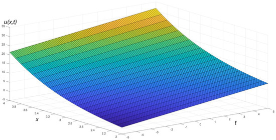
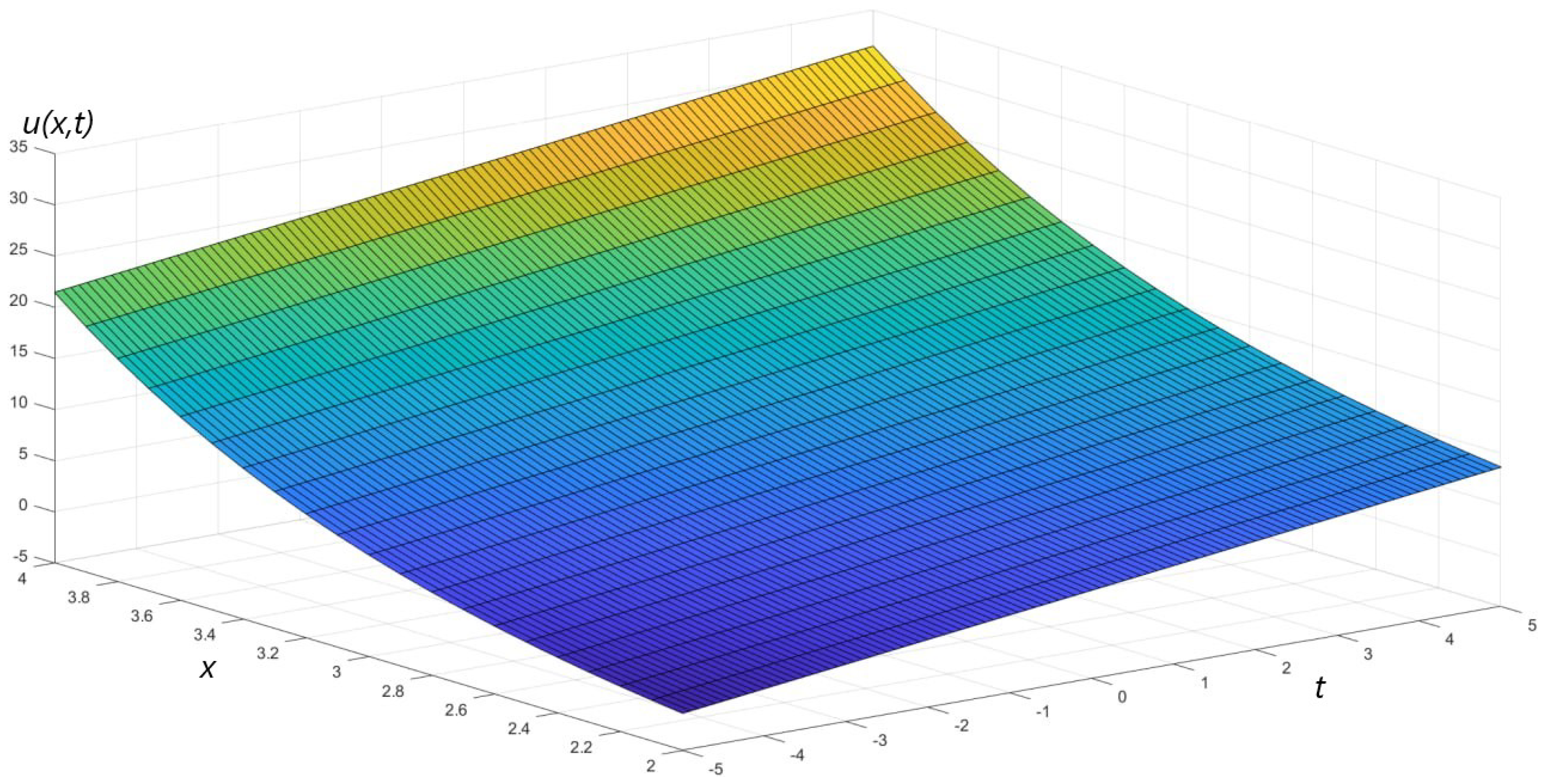
which is illustrated in Figure 1.

4. One-Dimensional Case with Oscillatory Source Term

Let $b\left(t\right)=1$, $\mu =1$, $G(x,t)=xsint$, and $\psi \left(x\right)=x+1$ in problem (3) and (4). We then consider the corresponding fractional-loaded equation

$${\displaystyle \frac{\partial z}{\partial t}}-{\displaystyle \frac{{\partial }^{2}z}{\partial x^2}}=J_{0,t}^{-\beta }z(0,t)+xsint,$$

(12)

$$z(x,0)=x+1,$$

(13)

where $J_{0,t}^{-\beta }$ denotes the Riemann–Liouville fractional integral operator of order $\beta >0$. By the integral representation derived earlier, we obtain the following.

$$z(x,t)={\int }_{-\infty }^{\infty }(\xi +1){\displaystyle \frac{1}{2\sqrt{\pi t}}}{e}^{-{\displaystyle \frac{{(x-\xi )}^2}{4t}}}d\xi +{\int }_0^{t}d\tau {\int }_{-\infty }^{\infty }\xi sin\tau {\displaystyle \frac{1}{2\sqrt{\pi (t-\tau )}}}{e}^{-{\displaystyle \frac{{(x-\xi )}^2}{4(t-\tau )}}}d\xi$$

$$+{\displaystyle \frac{1}{\mathrm{\Gamma }\left(\beta \right)}}{\int }_0^{t}d\tau {\int }_{-\infty }^{\infty }{\int }_0^{\tau }{(\tau -\eta )}^{\beta -1}z(0,\eta ){\displaystyle \frac{1}{2\sqrt{\pi (t-\tau )}}}{e}^{-{\displaystyle \frac{{(x-\xi )}^2}{4(t-\tau )}}}d\eta d\xi .$$

Introduce the standard decompositions

$$I_1={\int }_{-\infty }^{\infty }(\xi +1){\displaystyle \frac{1}{2\sqrt{\pi t}}}{e}^{-{\displaystyle \frac{{(x-\xi )}^2}{4t}}}d\xi ,I_2={\int }_0^{t}d\tau {\int }_{-\infty }^{\infty }\xi sin\tau {\displaystyle \frac{1}{2\sqrt{\pi (t-\tau )}}}{e}^{-{\displaystyle \frac{{(x-\xi )}^2}{4(t-\tau )}}}d\xi ,$$

$$I_3={\displaystyle \frac{1}{\mathrm{\Gamma }\left(\beta \right)}}{\int }_0^{t}d\tau {\int }_{-\infty }^{\infty }{\int }_0^{\tau }{(\tau -\eta )}^{\beta -1}z(0,\eta ){\displaystyle \frac{1}{2\sqrt{\pi (t-\tau )}}}{e}^{-{\displaystyle \frac{{(x-\xi )}^2}{4(t-\tau )}}}d\eta d\xi .$$

Evaluating the Gaussian integrals as shown in the previous example yields

$$I_1=x+1,I_2=x-xcost.$$

Reordering and evaluating the $\xi$-integral in $I_3$ gives

$$I_3={\displaystyle \frac{1}{\mathrm{\Gamma }\left(\beta \right)}}{\int }_0^{t}d\tau {\int }_0^{\tau }{(\tau -\eta )}^{\beta -1}z(0,\eta )d\eta ={\displaystyle \frac{1}{\mathrm{\Gamma }(1+\beta )}}{\int }_0^t{(t-\eta )}^{\beta }z(0,\eta )d\eta .$$

Hence, the integral representation reduces to the scalar Volterra equation

$$z(x,t)=1+2x-xcost+{\displaystyle \frac{1}{\mathrm{\Gamma }(1+\beta )}}{\int }_0^t{(t-\eta )}^{\beta }z(0,\eta )d\eta .$$

(14)

Setting $x=0$ in (14) yields the scalar equation for the trace:

$$z(0,t)=1+{\displaystyle \frac{1}{\mathrm{\Gamma }(1+\beta )}}{\int }_0^t{(t-\eta )}^{\beta }z(0,\eta )d\eta .$$

(15)

As in the problem considered in Section 3, the iterated kernels satisfy

$${\kappa }_1(t,\eta )={\displaystyle \frac{{(t-\eta )}^{\beta }}{\mathrm{\Gamma }(1+\beta )}},{\kappa }_2(t,\eta )={\displaystyle \frac{{(t-\eta )}^{2\beta +1}}{\mathrm{\Gamma }(2+2\beta )}},$$

and, by induction,

$${\kappa }_n(t,\eta )={\displaystyle \frac{{(t-\eta )}^{n\beta +n-1}}{\mathrm{\Gamma }(n+n\beta )}}(n\ge 1).$$

Truncating the resolvent after two iterates yields the approximation

$$\mathcal{R}(t,\eta )\approx {\kappa }_1(t,\eta )+{\kappa }_2(t,\eta )={\displaystyle \frac{{(t-\eta )}^{\beta }}{\mathrm{\Gamma }(1+\beta )}}+{\displaystyle \frac{{(t-\eta )}^{2\beta +1}}{\mathrm{\Gamma }(2+2\beta )}}.$$

Using this resolvent approximation and evaluating the resulting Beta-type integrals as in Section 3, we obtain the explicit representation

$$z(0,t)=1+{\displaystyle \frac{1}{\mathrm{\Gamma }(\beta +2)}}{t}^{\beta +1}+{\displaystyle \frac{1}{\mathrm{\Gamma }(2\beta +3)}}{t}^{2\beta +2}.$$

Substituting this expression into (14) and performing the termwise Beta-integral evaluations yields the expansion

$$z(x,t)=1+2x-xcost+{\displaystyle \frac{1}{\mathrm{\Gamma }(2+\beta )}}{t}^{\beta +1}+{\displaystyle \frac{1}{\mathrm{\Gamma }(3+2\beta )}}{t}^{2\beta +2}+{\displaystyle \frac{1}{\mathrm{\Gamma }(4+3\beta )}}{t}^{3\beta +3}+\cdots ,$$

(16)

where the displayed terms correspond to the first few iterates of the Neumann series for the Volterra operator.

In the classical integer-order case $\beta =1$, the expansion (16) reduces to

$$z(x,t)=1+2x-xcost+\frac{1}{2}{t}^2+\frac{1}{24}{t}^4+\frac{1}{720}{t}^6+\cdots .$$

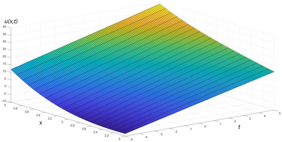
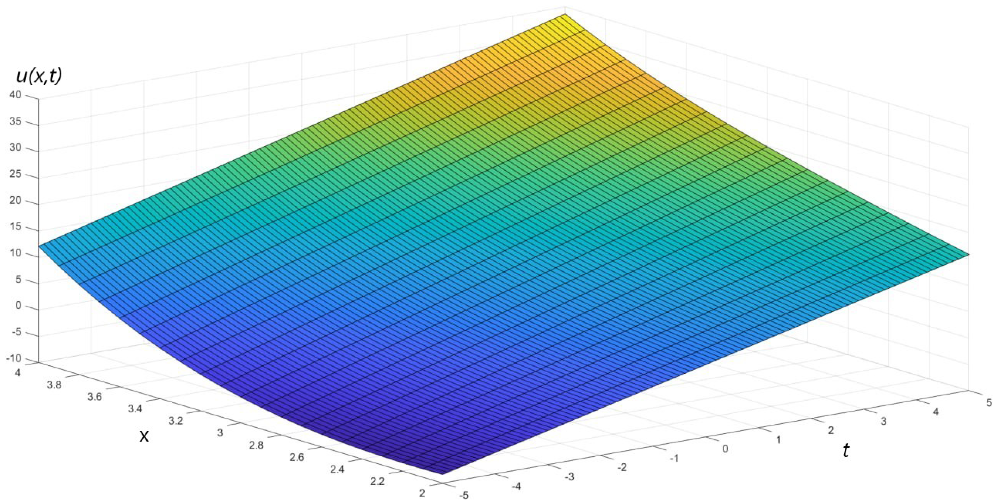
The corresponding solution profile is shown in Figure 2.

5. Conclusions

This paper investigated the Cauchy problem for a class of fractional intero-differential equations with a time-dependent diffusion coefficient and a Volterra-type memory term. By reformulating the original problem as an equivalent Volterra integral equation of the second kind, we established precise conditions under which the two formulations are equivalent and constructed the associated resolvent kernel.

This approach allowed us to derive explicit analytical representations of solutions in selected one-dimensional cases and to rigorously analyze their qualitative behavior. In particular, the results clarify the influence of the fractional-order $\beta$ and the loading term on the solution dynamics, highlighting the role of memory effects in comparison with the classical diffusion case. The graphical illustrations presented in Section 3 and Section 4 visualize the temporal evolution and spatial behavior of the obtained solutions. They confirm the analytical results and clearly demonstrate the smoothing effect of diffusion as well as the impact of the fractional order on the rate of propagation.

The proposed framework extends the classical theory of parabolic equations to diffusion models with nonlocal temporal effects and lower-dimensional loading terms. Possible directions for future research include extensions to higher-dimensional settings, nonlinear problems, and the development of numerical methods that preserve the kernel-based structure of the analytical solutions.

References

- Kosmakova, M.T.; Ramazanov, M.I.; Kasymova, L.Z. To solving the heat equation with fractional load. Lobachevskii J. Math. 2021, 42, 2854–2866. [Google Scholar] [CrossRef] [Scilit]
- Kosmakova, M.; Akhmanova, D.; Izhanova, K. BVP with a Load in the Form of a Fractional Integral. Int. J. Math. Math. Sci. 2024, 2024, 7034103. [Google Scholar] [CrossRef] [Scilit]
- Baltaeva, U.; Khasanov, B.; Egamberganova, O.; Hayitbayev, H. Well-posedness of problems for the heat equation with a fractional-loaded term and memory. Dynamics 2025, 5, 44. [Google Scholar] [CrossRef] [Scilit]
- Matrasulov, J.; Yusupov, J.R.; Saidov, A.A. Fast Forward Evolution in Heat Equation: Tunable Heat Transport in Adiabatic Regime. Nanosyst. Phys. Chem. Math. 2023, 14, 421–427. [Google Scholar] [CrossRef] [Scilit]
- Mukhamadiyev, A.; Urunbaev, J.; Bobokandov, M.; Rakhmonov, Z.; Khujakulov, T. A Self-Similar Analysis of the Solutions to the Cross-Diffusion System. Mathematics 2026, 14, 83. [Google Scholar] [CrossRef] [Scilit]
- Ntouyas, S.K.; Samei, M.E. Existence and uniqueness of solutions for multi-term nonlinear fractional integro-differential equations. Adv. Differ. Equ. 2013, 2013, 368. [Google Scholar] [CrossRef] [Scilit]
- Liang, Y.; Fan, Z.; Li, G. Existence, uniqueness and regularity of solutions for fractional integro-differential equations with state-dependent delay. J. Appl. Anal. Comput. 2024, 14, 623–641. [Google Scholar] [CrossRef] [Scilit] [PubMed]
- Yahia Awad, M.A.; Mghames, R.H.; Amin, K.M. Existence, uniqueness, and stability of solutions for nonlinear fractional integro-differential equations with nonlocal boundary conditions. TWMS J. Appl. Eng. Math. 2025, 15, 10–25. [Google Scholar]
- Li, Y.; Qu, B. Mild solutions for fractional non-instantaneous impulses integro-differential equations with non-local conditions. AIMS Math. 2024, 9, 12057–12071. [Google Scholar] [CrossRef] [Scilit]
- Agarwal, R.P.; Baleanu, D.; Nieto, J.J.; Torres, D.F.M.; Zhou, Y. A survey on fuzzy fractional differential and optimal control nonlocal evolution equations. Appl. Math. Comput. 2018, 339, 3–29. [Google Scholar] [CrossRef] [Scilit]
- Saldir, O. Numerical solution of fractional integro-differential equations with non-local conditions using reproducing kernel method based on Chebyshev polynomials. J. Appl. Math. Comput. 2025, 71, 1403–1431. [Google Scholar] [CrossRef] [Scilit]
- Durdiev, D.K.; Jumaev, J.J. Inverse problem of determining the kernel of an integro-differential fractional diffusion equation in a bounded domain. Izv. Vyssh. Uchebn. Zaved. Mat. 2023, 67, 1–13. [Google Scholar] [CrossRef] [Scilit]
- Agarwal, R.P.; Baltaeva, U.; Hubert, F.; Khasanov, B. Existence and uniqueness of the solution to initial and inverse problems for integro-differential heat equations with fractional load. Electron. J. Differ. Equ. 2024, 2024, 1–19. [Google Scholar] [CrossRef] [Scilit]
- Durdiev, D.K.; Elmuradova, H.B. Kernel determination problem in the fractional pseudo-integro-differential equation. Rend. Circ. Mat. Palermo 2024, 73, 3313–3326. [Google Scholar] [CrossRef] [Scilit]
- Alk-Kassab, K.; Al-Dahidi, I.; Dandach, A.; Al-Shawabkeh, A. Analytical and numerical treatment of evolutionary time-fractional partial integro-differential equations with singular memory kernels. Fractal Fract. 2025, 9, 392. [Google Scholar] [CrossRef] [Scilit]
Disclaimer/Publisher’s Note: The statements, opinions and data contained in all publications are solely those of the individual author(s) and contributor(s) and not of MDPI and/or the editor(s). MDPI and/or the editor(s) disclaim responsibility for any injury to people or property resulting from any ideas, methods, instructions or products referred to in the content. |
© 2026 by the authors. Licensee MDPI, Basel, Switzerland. This article is an open access article distributed under the terms and conditions of the Creative Commons Attribution (CC BY) license.