Spiking Neural Networks: History, Current Status and the Future

Abstract

Simulated spiking neural networks have been explored for over a hundred years. Many of these networks are driven by biological considerations and an attempt to simulate brains, but others are used with little biological consideration. This paper gives some history of the development of spiking neural models, their use for modelling biological and cognitive phenomena, and for machine learning. It introduces the current state of the art in computational biological neuron and synapse modelling and plasticity. It introduces and reviews balanced spiking networks and their engineering applications. Spiking networks are also used for machine learning, with the hope that their implementation on neuromorphic hardware will bring energy and time savings. Similarly, neuromorphic hardware can enable massive parallelism, supporting larger spiking networks. The use of spiking nets for machine learning, both with biologically plausible models and without, is discussed, showing that effective models already exist. The paper concludes with some notes about implementing spiking nets and a discussion including open questions and future work.

1. Introduction

Simulated spiking networks have been explored since at least 1907 [1], but are now becoming increasingly popular. Their use as models of biological neurons and networks of neurons has grown consistently for the last several decades, and, encouraged by recent deep network developments, their use as machine learning systems has grown very rapidly. Spiking nets are naturally parallel, and existing deep nets can be converted to spiking networks [2]. The spiking of neurons in biological brains is largely what makes them think [3].

This paper reviews work in spiking nets. Mostly, this work is in simulated spiking networks, but neuromorphic hardware is also used both for simulation and emulation, and it is included in this review. The review focuses on four major areas using spiking networks.

1.

Simulation of Biological Neurons and Networks;

2.

Balanced Networks;

3.

Neuro-cognitive Models;

4.

Machine Learning Systems.

While most of the networks called neural networks by computer scientists have continuously valued output, brains work with neurons that spike. Lapicque’s original model [1] was an integrate and fire model, and subsequently, there have been many models of spiking neurons (see Section 2).

While there have been many recent review papers on spiking networks (e.g., [4,5,6,7,8,9]), these almost uniformly are based around machine learning systems, though a few refer to control theory (e.g., [9,10]). Though balanced nets are used for control theory and machine learning, Majumdar [9] does not reference the basis of balanced nets, while Section 4 does. In addition to these, the current review provides an overview of the other two areas: simulation of biological neurons and networks, and neuro-cognitive models.

The paper is organised with the next Section 2 describing models of neurons, synapses, and plasticity. Next, the four major areas, biological simulation (Section 3), balanced networks (Section 4), neuro-cognitive models (Section 5), and machine learning (Section 6), are introduced. A section on implementation (Section 7) supports a reader implementing a spiking network. A broad discussion (Section 8), including questions and potential future work, is followed by the conclusion (Section 9).

2. Models of Spiking Neurons

Spiking neural networks are made up of neurons and synapses. Other units, such as glia, may be considered but are beyond the scope of this paper (Glia do play an important role. For instance, astrocytes, a type of glia, are involved in plasticity [11].). The basic neural model a system uses is important, and sometimes, multiple models are used in one network. Point models are simple and efficient (see Section 2.1), but less biologically accurate than more complex models (see Section 2.2). Section 7 describes some mechanisms for implementing spiking networks. Models of synaptic transmission (see Section 2.3) are divided into chemical and electrical synapses. Plasticity (see Section 2.4) is the basis of learning in spiking neural networks.

2.1. Point Models

The first spiking models were integrate and fire models [1,12], and they predate modern programmable computers. The neuron collects activation from other neurons that send synapses to it, integrating the activation. If it collects enough energy, it emits a spike. This can be done by a simple threshold or a dynamic threshold, or can be more stochastic, like a Boltzmann machine [13]. This is what a perceptron does [14]. However, unlike the earlier models, Rosenblatt [14] actually used perceptrons to develop systems that did some sort of computation.

Leaky integrate and fire (LIF) models are more biologically accurate. If neuron models are run in time steps, what happens to activation between time steps? Biologically, if a neuron does not spike, some of the activation leaks away, so more activation is needed to emit a spike in the next time step. A good example of this model is the generalised leaky integrate and fire model [15], but there are many other models. LIF models are currently the most widely used models of spiking neurons.

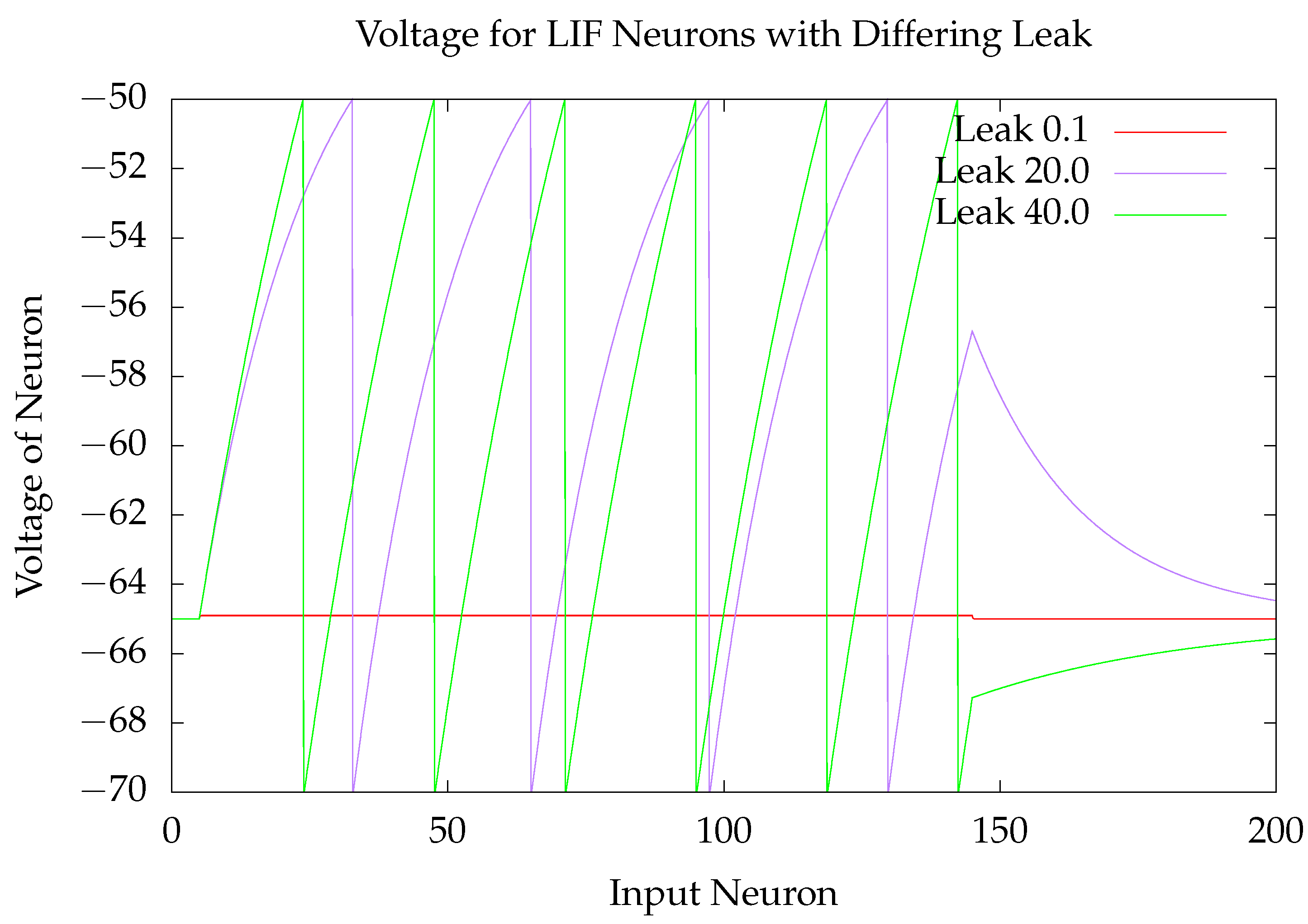
Figure 1 is an example of three LIF neurons. Each has the same input, a constant direct current from 5 ms to 145 ms. Leak varies, with the leak constant set to 0.1, the neuron is, in essence, an IF neuron that retains almost no energy from time step to time step (In the literature, this is called the leak constant, but it perhaps would be better to call it the retention constant because it actually reflects how much energy is retained.). In this case, there is a 0.1 ms time step. With the other two neurons, voltage increases until it reaches a threshold (−50.0) when the neuron spikes. After a spike, the voltage is reset (−70.0). At 145 ms, input stops, and leak returns the voltage to the rest setting (−65.0).

Another simple extension to the LIF model is adaptation. If a neuron spikes at a higher rate, it gets tired, like an overused muscle, and becomes more difficult to spike. It adapts. There are many good examples of LIF models with adaptation [16,17].

Another widely used point model is the Izhikevich model [18]. This is a reverberate and fire model. One of the benefits of this model is that it relatively accurately models a range of different types of neurons, though it can spike when inhibited too much. Biologically, there are bursting neurons, regularly spiking neurons, phasic spiking neurons and many other types of behaviour. The Izhikevich model manages all of these behaviours by setting two parameters. Note that the ability to account for different types of neurons is also shown by the generalised leaky integrate and fire model [15], and the Courbage–Nekorkin model [19]. Fortuna and Buscarion [20] provide a good review of neural models.

2.2. Complex Neural Models

The original Hodgkin–Huxley model [21] describes the neurochemical basis of a spike. It describes how the initial release of sodium leads to the neuron rapidly gaining voltage, followed by the release of potassium that lowers the voltage again. This has been extended to hundreds of models of neural behaviour and communication based on ion channels [22].

The behaviour of neurons is extremely complex, varies in time, and each neuron is unique. Biologists have developed a vast number of models with parameters, including neuromodulators and compartments. For example, one paper [23] describes a system where the neuron’s dendrite is broken into compartments; depending on where synapses arrive on the dendrite, different behaviour occurs, and this system accurately simulates the biological behaviour of in vivo neurons. Particular models are available for reuse. One model is a common basis for a particular pyramidal neuron [24]. Dendrites have been widely studied over the last two decades, with one study showing the impact of dendrites on spiking behaviour [25].

One of the potential benefits of spiking neural systems is that they can be implemented in neuromorphic hardware (see Section 8.1). Threshold selectors with tunnel diodes [26] have been used as neural models, which are easily implemented in hardware. Similarly, Josephson junctions are also readily implemented in hardware [27,28].

2.3. Synapses

Models often contain a separate component for synapses: the connections between neurons. Synapses can be divided into two types: chemical synapses and electrical synapses. Though both synaptic types are electrochemical, those termed chemical have a synaptic cleft, while the neurons actually physically touch in electrical synapses.

There is a reasonable understanding of the biology of chemical synapses [29]. Simple models of chemical synapses manage the current that is passed over the synapse over time, with those chemicals passing over the synaptic cleft. In a simple simulated system, a synapse has a weight, and that weight is passed over the synapse from the pre-synaptic neuron to the post-synaptic neuron when the pre-synaptic neuron spikes. Two common time profiles include: exponential decay, which, after an initial rapid increase of rate, decays at an exponential rate, and the alpha function [30], which initially rises at a slower rate, then decays.

Electrical synapses [31] are less widely simulated, and perhaps less widely known. Direct connections between neurons enable ionic current to flow directly between neurons. Interaction between electrical and chemical synapses [32] is an active area of biological research. For example, gap junctions, a type of electrical synapse that occurs in the retina, are well studied [33]. They are dynamically regulated by circadian rhythms. They have a number of functional roles, for instance, transfer of visual signals in cones. There is also evidence that gap junctions between inhibitory neurons support synchrony [34].

2.4. Plasticity

Perhaps the main benefit of spiking neural nets is their ability to learn. Learning can be broken into three major types: long-term plasticity, short-term plasticity, and structural plasticity. Long-term and short-term plasticity refer to changes in the weights of synapses.

Most work in the simulation of plasticity has been devoted to long-term plasticity. Biologically, this weight change persists for a considerable duration [35], but in simulation, the weight change is typically permanent.

One long-standing form of learning is called Hebbian learning [36]. If a neuron tends to cause another to spike, the synaptic weight is increased. There are many variants of this rule: the BCM rule [37] is widely used, and Oja’s rule [38] sets the weight to the likelihood (over past behaviour weighted to recency) that the pre-synaptic neuron causes the post-synaptic neuron to spike.

Spike timing-dependent plasticity (STDP) is a form of Hebbian learning that has significant biological support [39,40]. The basic idea behind STDP is that the weight increases when the pre-synaptic neuron spikes before the post-synaptic neuron and decreases when it spikes after. There are many STDP rules, including rules that are based on three spikes [41] and a symmetric rule combined with synaptic scaling [42,43]. Some of these have little biological evidence to support them.

Hebbian learning mechanisms are often compensatory [44]. An early concern of Hebbian learning mechanisms was that the synaptic weight could grow without limit. This could be capped, but then many synapses would typically go to the cap. Instead, compensatory rules limit the amount of total synaptic weight entering or leaving a neuron (or a combination of both). Oja’s rule [38] is an example of this. Compensatory mechanisms force the synapses to compete for synaptic weight.

Again, there is no reason to insist on biological plausibility. Indeed, one of the main current motivations for spiking nets is for machine learning applications (see Section 6). It is not possible to directly translate the backpropagation learning rule or other gradient descent methods to spiking nets because they depend on a differentiable transfer function; that is, the error gradient that the system is learning to descend. The spikes are not differentiable, but proxies can be used. A common proxy to use is the voltage of the neurons [45].

Short-term plasticity changes the weight of a synapse for a relatively short duration, which typically varies from seconds to hours. After the initial weight change, the synaptic weight slowly reverts to its original weight. The Tsodyks–Markram rule is widely used [46]. Depending on the parameter settings, the synaptic weight increases (or decreases) as the pre-synaptic neuron spikes. It then gradually reverts to its base weight over time. This is consistent with the vesicle depletion model and is not Hebbian [47]. There is evidence for Hebbian short-term plasticity [48].

It should also be noted that it is possible to combine several different learning rules [49]. This combination can lead to improved overall behaviour.

While long and short-term plasticity change the weights, or fine topology, another form of plasticity changes the gross topology. This structural plasticity adds and removes synapses, and adds and removes neurons. Biologically, the brain starts with the first neuron and adds and removes neurons and synapses throughout life. Ongoing structural plasticity includes Hebbian and anti-Hebbian paradigms, but is also used for homeostasis [50].

3. Biological Models

The domain that uses spiking nets most widely is probably biological modelling, and it is certainly the domain that has used them longest. Lapicque’s integrate and fire model [1] was introduced in 1907 as a biological model. Developments have continued throughout the intervening century, with notable examples including McCulloch and Pitts (1943, another variant of integrate and fire) [12], Hodgkin and Huxley [21] (1952, a model that explains the neurochemistry of a spike), and the Morris and Lecar model [51] (1981, a neurochemical model of neuron behaviour).

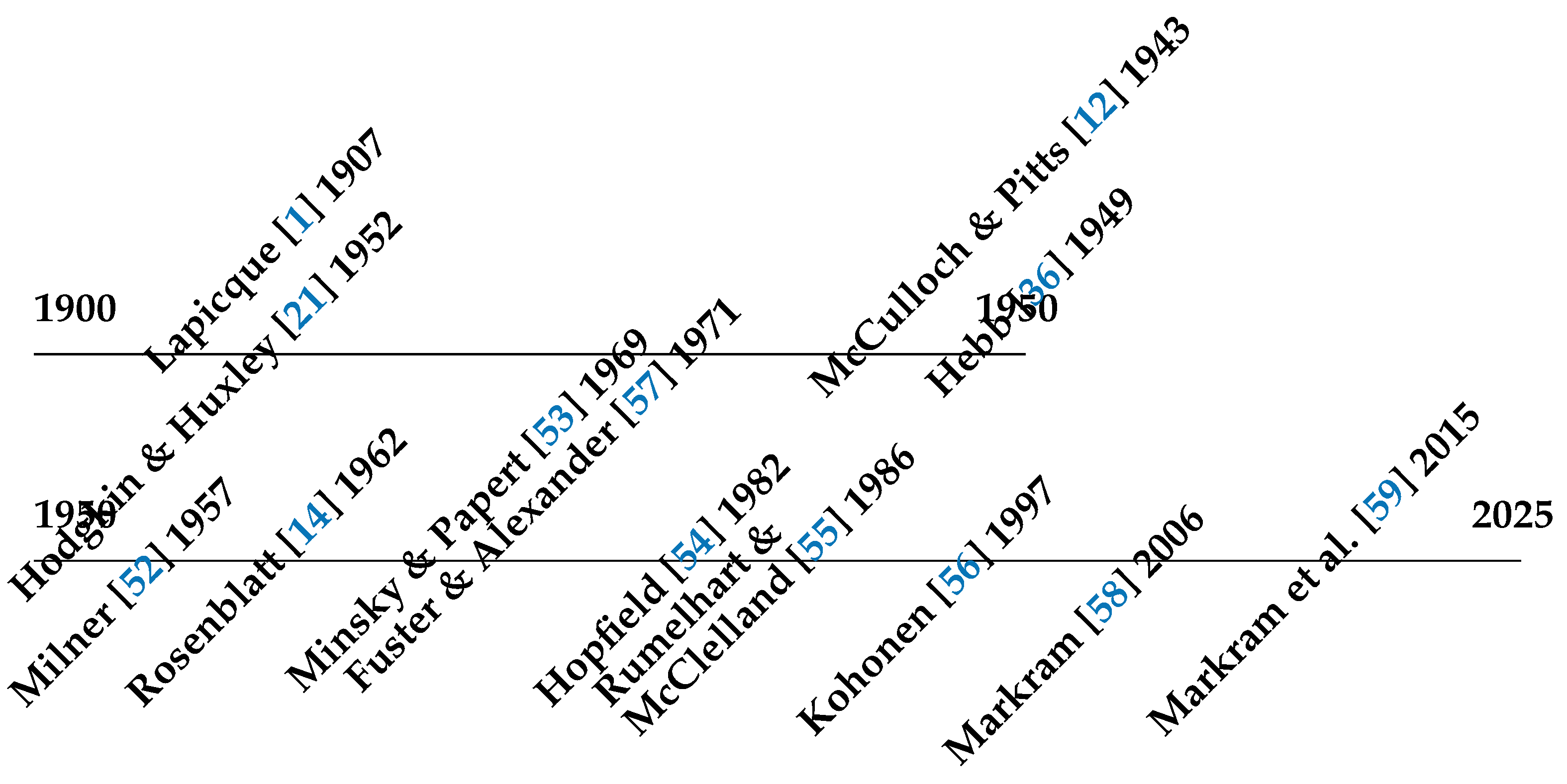
Figure 2 places some of these important models and other significant papers on a timeline. The timeline includes several spiking models [1,12,21] that directly connect biology to simulation. Hebb [36] introduces cell assemblies (see Section 5.2) and Hebbian learning, introducing neuropsychology, and this is extended by Milner [52], introducing inhibitory synapses. Rosenblatt [14] uses point models (perceptrons) for actual calculation and indeed learning, though the learning rule is later shown to be incomplete [53]. There is not a good understanding of how neurons actually generate cognitive behaviour. Connectionist systems, including Hopfield nets [54], multi-layer perceptrons [55], and self organising maps [56] have furthered understanding of neural and connectionist computations. Seminal work in biology is also important, with Fuster and Alexander [57] presenting solid evidence of the involvement of particular neurons in a cognitive task. The implementation of a computational model of a spiking net of an entire human brain was proposed in [58]. Finally, a large-scale (though still far from complete) fine-grained neuron simulation [59] shows recent large-scale simulation work.

Neurons in brains spike. Simulated spiking neural networks can be developed as in silico models of brains, areas of brains, or neural circuits. Increased fidelity of the neural, synaptic and plasticity models improve the accuracy of these networks as models of the underlying biological neural system.

Biologists are interested in how neurons work. Fortunately, it is reasonably simple to see how a single neuron works both in vivo and in vitro. On the other hand, neurons themselves (like all cells) are incredibly complex, so understanding of how a biological neuron works is still incomplete. Of course, each neuron is unique and is constantly changing. Biologists are addressing these issues by building more and more realistic models of neurons and neuron circuits [60].

Short-term and working memory are examples of a biological answer to a psychological question. How do neurons support short-term memory? Hebb’s cell assembly proposal ([36], see Section 5.2), is a hypothesis, but it is supported by relatively early single unit recording work [57] that supports the hypothesis. This is an early example of linking biological spiking behaviour to cognitive phenomena. Simulations with spiking neurons [61] support this model.

A recent system develops a form of reinforcement learning based on the dopamine system [62]. Experiments on mice show how this mechanism reflects behaviour in their midbrain.

Biological spiking models can generate precise models of neural behaviour. For example, Markram et al. [59] show a simulation of 30,000 neurons representing ${0.3}^3$ mm of the cortex. This simulates a range of spiking patterns that occur in actual human brains. This shows both the promise of simulating an entire brain in spiking neurons and the challenge of scaling from 30,000 neurons to 85 billion.

This paper [59] arises from several research groups that worked on the Human Brain Project [63]. This large project was related to an earlier proposal, the Blue Brain Project [58] that hoped to simulate an entire brain on supercomputers. To this point, the Blue Brain Project has, as yet, been unsuccessful. There are several reasons for this, but one obvious reason is that it is computationally expensive to simulate the roughly 85 billion neurons [64] in a typical human brain with reasonable fidelity.

Computational spiking models are good for models of relatively small brains, such as C. elegans [65]; even at this level, models are far from complete, as development and a dynamic environment are difficult to simulate. As noted above [59], spiking models are good for restricted, relatively small areas of brains, even human brains. Spiking models are also good for accounting for the behaviour of particular neurons in particular experimental settings (e.g., [66]). Finally, spiking models are good for showing that certain computations can be implemented in spiking neurons, and thus in brains (e.g., [67]).

Spiking neuron computational models of neurobiological processes are a very broad and active area of research [68]. A full review is clearly beyond the scope of this paper. Hopefully, links to further reading here are sufficient to aid further exploration.

4. Balanced Networks

Spiking networks with each neuron having roughly balanced inputs and outputs have been explored [69] in a biologically motivated study that shows chaotic spiking behaviour, though the overall number of spikes is linearly related to the number of inputs. This behaviour at the edge between stability and instability is studied in biology in, for instance, the auditory system [70].

Spiking networks that simulate biological models are constrained by the physical behaviour of the network they are simulating. There is no practical reason for this limitation in general, and balanced networks often take advantage of this.

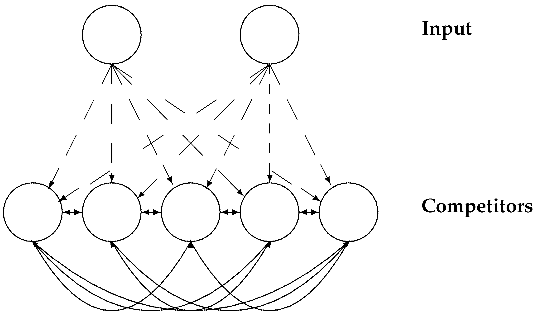
Using a mathematical model of a spiking network [71] with instant synaptic transmission, a winner take all (WTA) network can learn to maximise expectations using Hebbian synaptic plasticity. This WTA model is a balanced net with only one neuron spiking at a time. This is used for machine learning (see Section 4.2). An example of this topology is shown in Figure 3.

It is important to note that this is not a sound biological model and uses many mechanisms that are not biologically plausible. First, infinite speed of synaptic transmission is clearly impossible. Second, the neural model that is used has a type of adaptation that has little biological evidence. Finally, the synaptic connectivity requires each categorisation neuron to inhibit all of the others, which is not seen in biological systems.

4.1. Control Theory

The chaotic nature of balanced nets enables them to be used to simulate arbitrary linear dynamical systems. One simulated spiking net uses fast and slow synapses [72,73]. The connectivity matrix is calculated based on the desired target dynamical system. Input from the environment of the target system is translated into a direct current source in the spiking system. The output spikes are, similarly, translated to the output of the target system. Depending on the number of neurons in the system, the spiking system’s output accuracy varies, becoming more accurate as the number of neurons increases. This system can be used, for instance, for robotic control. The target dynamical system has sensors as input, and effectors take the output to control the robot. A cart and pole target system is one simple example.

Other spiking mechanisms are used for control. Above, Boerlin et al. [72] derive a proportional integral derivative (PID) system based strictly on spiking neurons. Spiking PIDs can be extended by, for example, neuroendocrine-inspired systems [74], BELBIC controllers, and other modifications. See Sepulchre [10] for a review.

An interesting spiking net comprehensive review paper [9] mentions control theory without actually unpacking balanced networks. It does have mistakes; for instance, it implies that the STDP learning rule is not Hebbian. Since it only applies when the pre-synaptic neuron fires before the post-synaptic neuron, the pre-synaptic neuron not only tends to cause the post-synaptic neuron to fire, it, at least partially, causes the neuron to fire.

4.2. Machine Learning with Balanced Networks

Another example of balanced networks is for machine learning. (For other types of machine learning with spiking nets, see Section 6). The original work by Habenschuss et al. [71] had an example with a machine learning task.

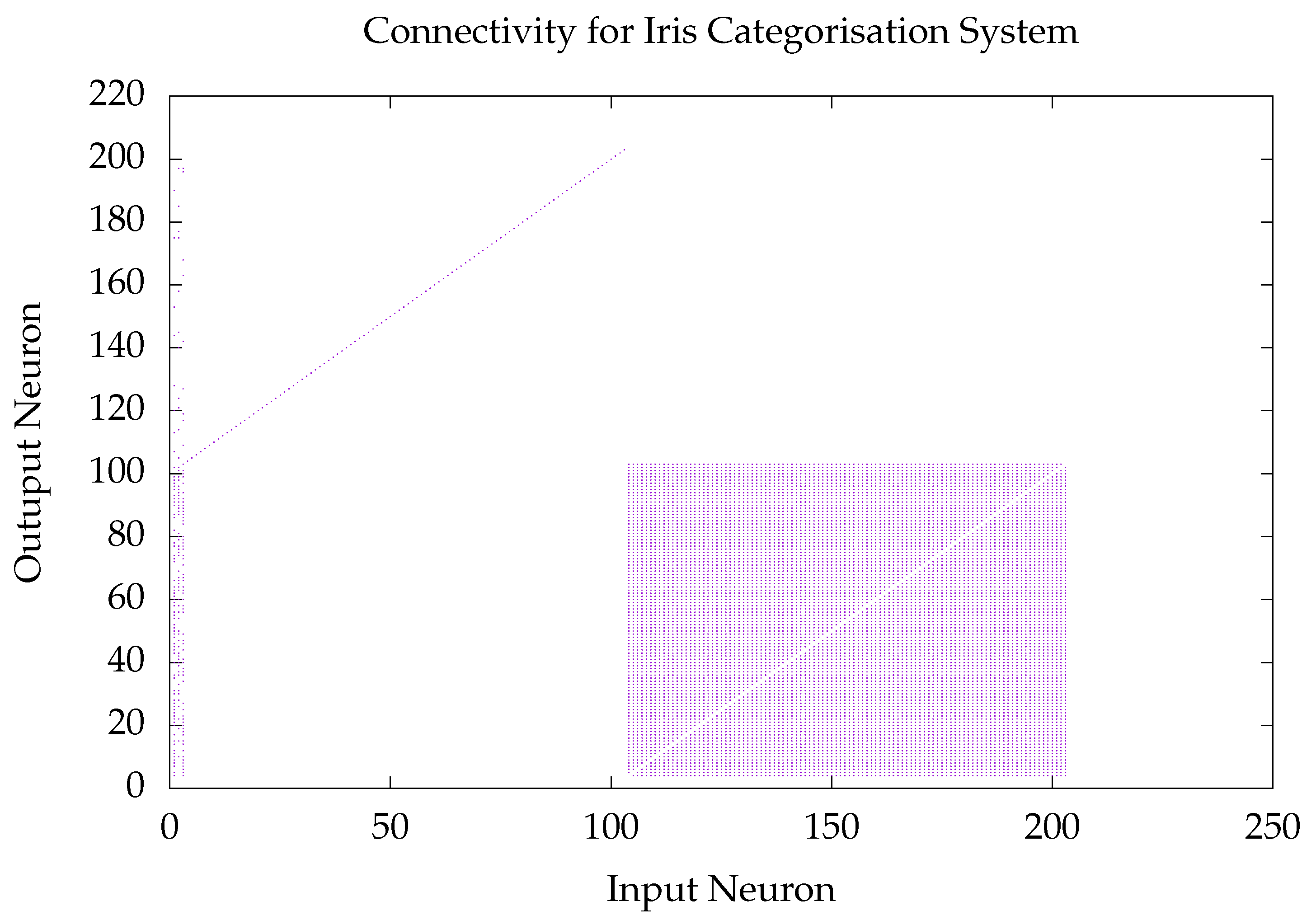
This work was expanded to include inhibitory and excitatory neurons [75]. Both systems learned with a form of STDP. The basic idea of the topology is that there are categorisation neurons stimulated by input neurons via plastic synapses, and inhibitory neurons stimulated by static synapses from the input neurons. The input neurons are stimulated to reflect the data. A connectivity matrix for an example of this system can be seen in Figure 4. It is from an example of an Iris [76] categorisation system, with four input neurons, 100 excitatory categorisation neurons, and 100 inhibitory neurons. Note that each categorisation neuron has a synapse to its paired inhibitory neuron, and each inhibitory neuron connects to all of the other categorisation neurons. The connections from the input neurons are stochastically generated, with each input connecting to 70% of the categorisation neurons and 30% of the inhibitory neurons.

Additionally, the time course of synaptic transmission varies from input neurons to the categorisation neurons and the inhibitory neurons. There are constant delays, but they vary from synapse to synapse. For instance, these can vary from between 1 and 10 ms. This delay supports the distribution of categorisation neurons in the input space, so that some are more likely to respond first on particular inputs, and learning supports the differentiation.

It is an unsupervised learning mechanism. There is a one to one relationship between the excitatory and inhibitory neurons, with the excitatory neurons stimulating their own inhibitory mate, and the inhibitory neurons inhibiting all of the other excitatory neurons. If the speed of synaptic transmission is instant, the behaviour is the same as the original topology from Figure 3. The excitatory category neurons respond to particular input instances, and the STDP makes the weights stronger so that they, in essence, move toward the input instance in the feature space. After training, the excitatory neurons are labelled with the category of the inputs to which they respond. To categorise, learning is turned off, and new data is labelled based on the category of the neurons that respond to the input data.

5. Neural Cognitive Models

Ideally, the scientific community would already understand how all 85 billion neurons in a particular human brain behave. However, the community is not even close to understanding how all of those neurons behave, or even how many neurons there are [77]. It is possible to see the spiking behaviour of perhaps ten thousand neurons in real time [78], and there are several imaging modes (e.g., fMRI [79] and EEG [80]) that show how relatively large areas of the brain behave in real time, but not the spiking behaviour. There is a poor understanding of how any neurons come to behave as they do.

If the community understood how all the neurons behaved, the process of understanding how the neural behaviour mapped to psychological behaviour could be easily explored, and the development of full-fledged neuro-cognitive models could begin. Simulations are useful, though a Blue Brain-like system [58] could not currently behave in anything like real time.

Instead, spiking neuro-cognitive models are currently quite simple. Spiking models use a relatively small number of neurons, and many assumptions, either implicit or explicit, are made. Research in neuro-cognitive models has been ongoing for over 150 years [81], and a wide range of connectionist mechanisms has been used for cognitive modelling. Interactive activation models [82] have had many cognitive models implemented in them since the 80s. Multilayer perceptrons were also used [83]. Recently, large language models have been used as cognitive models [84]. However, spiking neuro-cognitive models are less popular while still obviously being closer to the actual neural basis of cognition.

An early spiking cognitive model [66] accounts for short-term memory. The neurons correlate with biological neurons from the monkey cortex. Probabilistic spiking neurons are used, and the simulated neuron behaviour is mapped to the biological behaviour recorded while the monkeys perform a visual delayed matching task. The simulated neurons are connected so that there are several attractor states, and they spike similarly to the biological neurons while performing the same task. Even in 1993, Zipser et al. [66] account for the behaviour of 176 of 179 biological neurons with a one-to-one mapping of the behaviour of their simulated spiking neurons. A more recent system [85], using a ring attractor of spiking neurons and short-term plasticity, also implemented a working memory system.

One well-explored system uses a vector space representation [86,87]. A real valued vector is calculated from the spiking behaviour of neurons associated with each individual element. Particular operations can be performed on the vectors to create output vectors. For example, natural language sentences can be parsed and lists can be memorised.

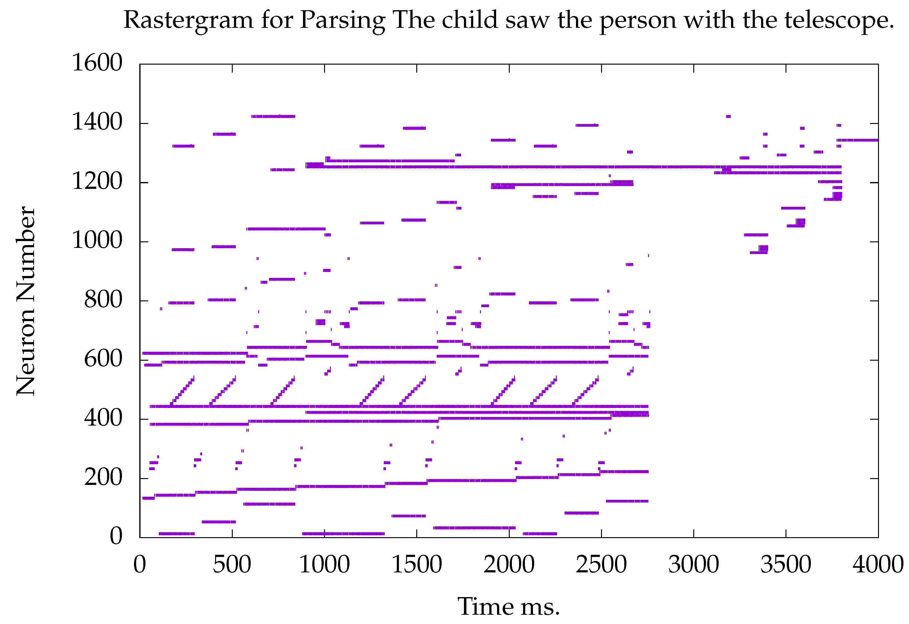
Another model of natural language parsing [88] uses spiking nets to parse context-free languages. Binding is performed by short-term potentiation, stacks are avoided by using memory-based parsing [89], and an overall mechanism for task domain separation (e.g., semantics, and syntax) is followed [90]. Semantics are implemented and used to resolve prepositional phrase attachment ambiguity. Parsing is done in psychologically realistic times. A rastergram of a parse of the sentence "The child saw the person with the telescope." is shown in Figure 5.

Note that the reproducibility of a spiking neural net depends on the technology in which it is implemented. For instance, running a model in the Nest [91] simulator is deterministic if the underlying neural model has no randomness. On the other hand, randomness is inherent in many neuromorphic systems (e.g., BrainScaleS [92]). Nonetheless, this randomness can be probabilistically accounted for and can indeed lead to better overall behaviour.

5.1. Attractor Networks

An attractor network is a system where each unit moves to a largely stable state. The canonical example is a Hopfield net [54], where each unit is connected to every other unit with bidirectional weights. In each time step, each unit can be either on or off. If it is on, it spreads weight to the other neurons based on the weight of their connection. When the system is started in an initial state, it will move stepwise to a stable state where each unit remains in the same state. A net of N units can have N attractor states, and the states can be stored via a type of Hebbian learning.

Attractor networks were widely used in the 1980s and 90s [93]. In this case, the units were considered neurons, as they are roughly integrate and fire neurons. This work was widely used to show the capacity of memory systems, with the capacity being that a network of N units could hold.

5.2. Cell Assemblies

The cell assembly (CA) [36] hypothesis is that many concepts in the brain are represented by a small number of neurons that have high mutual excitatory synaptic strength. For example, the concept dog is represented by a CA, and when the person is thinking of a dog, that CA becomes active by its neurons spiking at an elevated rate. While it is spiking, it is in short-term memory, and it can persist after the initial presentation ceases. Hebb [36] did not have solid evidence for inhibitory synapses when he proposed the CA. Milner [52] extended the theory to include inhibitory synapses after biological evidence had emerged.

There is evidence that CAs exist in all cortical areas and several subcortical areas [94]. Buzsáki [95] proposes a broad mechanism for using CAs for cognitive computation, which is consistent with a more modern focus on neural networks than on neurons alone [96].

One spiking system [97] learns to represent words across areas that are considered representations of cortical areas. The words are learned via a Hebbian rule, and there is some evidence that neurons in these areas are used to represent these words [98]. CAs are also widely used in neurosymbolic reasoning [99]. A great deal of work has been done in symbolic reasoning, and CAs provide a basis for symbols in spiking neurons.

It is noteworthy that much of the CA modelling assumes a single attractor state or one where the neurons in the activated CA all spike at an elevated rate as long as the memory is active. A different model [100] suggests that instead, there are circuits with neural firing that pass through different areas of the brain, then return to the original area. This is related to synfire chains [101].

One review of working memory [102] describes several different mechanisms to support working memory. The classic model uses the CA hypothesis, with the current working memory item spiking at an elevated rate. This can be extended with short-term plasticity. For example, Fiebig and Lansner [67] show a simulation of working memory supported by short-term potentiation. Again, an alternative allows the memory to flow around a circuit, such as thalamocortical circuits [100] or cerebrocortical circuits [103]. It is possible that some CAs are implemented in the classic model, and others in the circuit model.

6. Machine Learning

One of the main benefits of neural nets in general, including spiking nets, is that they can learn. There is a great deal of interest in learning with spiking nets. Research in this area can be divided into biologically plausible systems (Section 6.1), gradient descent methods (Section 6.2), and reinforcement learning (Section 6.3).

One question that is common to all these methods is how the inputs are provided to the system. This can be done by converting input vectors into spikes, or just into current. Another method is that each feature value pair can be represented by an input, but this method can lead to a large number of input features. Nunes et al. [6] provide a discussion of how spiking nets are used in machine learning.

6.1. Biologically Plausible

To some extent, the balanced models from Section 4.2 are biologically plausible. The topology is not entirely biologically reasonable, but it does work with several STDP rules. Taherkani et al. [4] have a good review of learning in biologically plausible nets.

One system uses recurrent networks to develop cell assemblies that respond to appropriate categories [104]. A compensatory Hebbian learning rule is used, and the network is broken into four subnetworks: presentation, first intermediate, second intermediate, and categorisation. All but the presentation subnets have recurrent synapses, and there are forward synapses through the subnets. There are backward synapses through the net, but not to the presentation subnet. All synapses are plastic. During training, activation proceeds from input and categorisation neurons to the two intermediate subnetworks. Novel input is categorised by the spiking behaviour of the categorisation neurons, when a novel input vector stimulates the presentation subnet.

Typically, learning is done by adjusting synaptic weights using Hebbian learning rules. The most widely used and a well-supported mechanism is STDP (see Section 2.4). Another important issue is timing. With STDP, the timing of spikes is crucial. The balanced network systems (Section 4.2) gain initial diversity of categorisation neurons from having the timing of spike arrival vary from synapse to synapse.

Another type of learning, anti-Hebbian learning, is also widely used. Here, neurons that spike at similar times have their synaptic weight reduced. This leads to a diversity of spiking behaviour [49].

In the medium term and beyond, there is hope that spiking learning systems can take full advantage of the highly recurrent nature of networks in the brain [105], and of their long lasting nature. This will lead to systems that are appreciably more human like.

6.2. Gradient Descent

In 1969, progress in machine learning with neural nets was slowed when it was noted that the standard learning rule at the time, the perceptron learning rule, could not learn the simple exclusive or function [53]. This was resolved over a decade later, when the PDP books [55] introduced learning by backpropagation of error. With backprop, multi-layer perceptrons could change the connection weights by descending the error gradient in a supervised manner.

Gradient descent is a supervised mechanism that does not seem to appear in brains, so it is not biologically plausible (There is evidence of error signals in sensory areas [106], but the signal is not a direct signal to adjust synaptic weight.). Moreover, gradient descent is difficult to perform on spiking networks, because spikes are not differentiable; it is not entirely clear how to descend the error gradient because the output of neurons is not a differentiable value.

One method used for gradient descent is SpikeProp [107]. It bases the error on the time that spikes are emitted. If the ultimate value is too low, the spike needs to be earlier, and if too high, it is later. Another uses multiple spikes [108]. A third makes extensive use of the underlying neural model in calculating the error gradient [109]; this yields results in the range of 99.36 ± 0.05% on the MNIST task.

Another mechanism is to entirely avoid learning in spiking nets and learn in standard artificial networks. Once the learning has been done, the network, along with weights, can be converted into a spiking network. One example [2] merely translates the learned deep net from continuously valued neurons to spiking neurons. On the standard MNIST task using unsupervised learning, Diehl and Cook’s [75] achieved 95% (see Section 4.2), and Diehl et al. [2] managed 99.1% using the conversion method.

Another example endeavours to reduce the number of spikes emitted [110] to make the system more energy efficient, perhaps based on neuromorphic hardware (see Section 8.1). A review article on deep learning with spiking neurons [111] is pertinent.

Another recent review paper [7] discusses deep spiking nets. This paper focuses on feed-forward deep network topologies that are not biologically plausible and is not concerned with other aspects of biological plausibility. It is a solid review and is useful for further exploration of spiking deep nets. However, it does not consider biology (Section 3) or psychology (Section 5), unlike the paper you are currently reading.

Other mechanisms exist, such as Liquid Time-Constant Networks [112]. Hasani et al. [112] use continuously valued output neurons and back propagation through time, but Contreras et al. [113] use a spiking Liquid Time-Constant Net. This is used to categorise seizures from EEG data. Another hybrid spiking architecture [114] is inspired by corticohippocampal circuits and learns in dynamic environments using the circuit model of brain function [100]. This combines continuously valued neurons and spiking neurons to develop systems that resist catastrophic forgetting in complex categorisation tasks.

6.3. Reinforcement Learning

Unlike supervised learning, reinforcement learning does not require the correct answer, but instead depends on the result of the action. If the result is positive, the action is rewarded, and if negative, it is punished. This can be implemented with biologically plausible mechanisms.

For instance, spiking neurons using STDP can be used for reinforcement learning. One system [115] uses an actor–critic framework to allow the agent to solve a simulated water maze task.

Another instance of reinforcement learning [116] is implemented on Loihi [117], a neuromorphic platform. This uses a deep reinforcement network to perform a robotic navigation task and uses less than a hundredth of the energy of a non-spiking implementation.

While the standard learning mechanism is used to adjust syntactic weights, another mechanism is used to adjust neural parameters (for instance [118]). Of course, synapses are part of the pre and post-synaptic neuron, so they are neural parameters, but standard thinking separates the two. This is explored in a sound review [8] (that also has interesting references to neuromorphic platforms).

7. Implementation and Running Spiking Nets

It is relatively easy to implement and run spiking nets on standard hardware. One can build a simulator from scratch, or take advantage of several commonly used simulators, for instance, Nest [91], Brian [119], or Neuron [120]. A second option is to use simulator-independent middleware, PyNN [121]. This builds the neural network topology and the input–output mechanisms, then calls the simulator. The same system can then be used on different simulators or on some neuromorphic hardware.

A third option, frequently used with balanced nets, is to use a mathematical package. For example, Matlab [122] is often used.

An open source platform [123] is available for implementing machine learning applications in spiking nets. There are mechanisms to build functional networks with spiking neurons [124]. Indeed, spiking nets are Turing complete. A useful review of strategies [125] can provide other pointers.

There are also visualisation tools for spiking nets. A simple tool is to make a rastergram that shows the spikes of each neuron. An example from a parser (similar to that shown by Huyck [88]) is shown in Figure 5. The parse has the neurons representing the words at the bottom, and those representing the semantics at the top. The parse stops around 2750 ms, and the semantic output is retrieved from the verb frame. The verb frame is the long line around neuron 1250, the only neurons to persist in spiking beyond the parse. The stripes represent reverberating cell assemblies that fire persistently until turned off. When particular CAs are understood, the change of the system’s state is clear. In this case, it shows that the semantics of the sentence are retained after parse completion with the telescope as the instrument of saw.

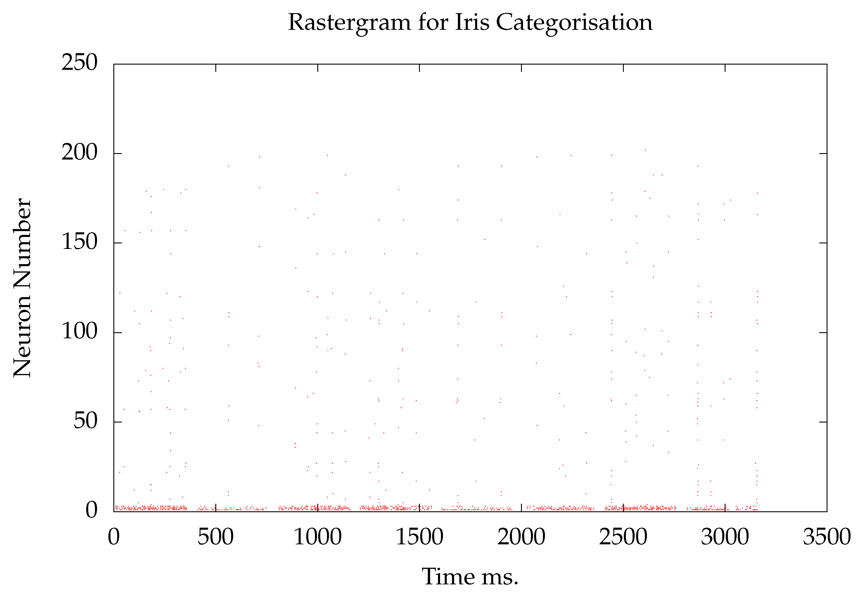
Similarly, Figure 6 represents the 204 neurons involved in an Iris categorisation [76] system. The bottom four neurons present the features from the data set, and these fire quite frequently. The categorisation neurons (the next 100) and the inhibitory neurons (the top 100) fire quite infrequently, which is the basic premise of a balanced network. Note that in this case, the rastergram is displaying about 6 million data points, and, in Figure 5, 32 million.

A recent review article on applications of spiking nets [5] notes that spiking nets can run on neuromorphic hardware that promises to be more efficient and energy-wise, than, for instance, deep nets running on standard hardware (see Section 8.1). Spiking network development in PyNN enables simulation in Nest on a standard PC. The same system also runs on SpiNNaker. SpiNNaker runs appreciably quicker on large simulations, for example, those with over 5000 neurons.

8. Discussion

One particularly important aspect of spiking systems is that they are parallel and they can be implemented in parallel hardware; see Section 8.1, which discusses the advantages of parallelism, and the use of neuromorphic systems for running spiking networks. This paper has been biased toward the author’s own background, which has the goal of pursuing AI; Section 8.2 discusses how spiking nets can be used to further understand cognition, and to work toward Turing test passing AI. Section 8.3 describes several spiking net projects that could be explored in the immediate future.

8.1. Parallel Processing and Neuromorphic Computation

Each neuron is a processor, so spiking nets are vastly parallel. As Moore’s Law seems to be running out, parallel computation is a growing field of interest. While neurons do depend on each other for input and output, and spiking nets can have neurons that function in sequence, simulated spiking nets are certainly able to function in parallel. Biological neurons may influence each other in manners different from synaptic connections, but to a large extent, synapses aside, they function independently. Neuromorphic systems are one mechanism for parallel processing. Neuromorphic systems like Loihi [117], BrainScaleS [92], and SpiNNaker [126] are highly parallel.

I have made a fair bit of use of SpiNNaker [126]. I have my own board (for under a million neurons), but the billion neuron system is available for remote use. It uses standard VonNeumann chips, but a massively parallel amount with 1000 neurons typically running in real time on each core. What is really clever about the system is the message passing algorithm and underlying hardware that enables the spikes to be passed to the appropriate neuron on the appropriate core in one millisecond.

Unlike earlier vector processing parallel systems, each neuron is computing something different. While it is relatively easy to convert these spikes into standard parallel computation, what is really interesting is to understand how the brain is calculating in parallel. Moreover, there are questions of how general spiking nets can calculate in parallel independently of how brains calculate. For instance, it is not clear that balanced nets (Section 4) are (or are not) being used in the human brain. Nonetheless, those computations can be performed in spiking nets, and they can be performed on neuromorphic hardware.

One benefit of spiking nets is that communication is done by one mechanism, spikes. If a subsystem is developed, it can communicate with any other subsystem by spikes. This has engineering benefits.

Another benefit is that neuromorphic systems can be readily integrated with event-based sensors. For example, neuromorphic cameras are integrated with Loihi to recognise gestures [127]. These event-based cameras are close to biological vision that only leads to spikes when the visual scene changes.

Developing systems with spiking nets is an odd way of programming. Computer scientists can readily develop serial systems, but developing parallel systems in general is much more difficult [128]. Working with spikes is another level of complexity, and learning makes this even more complex. Moreover, there is a real problem that the academic community does not understand how the brain computes. Like balanced networks, mechanisms such as Hopfield nets [54] and self-organising maps [56] enable more sophisticated computation with spiking nets.

It should be noted that both Hopfield nets and cell assemblies (Section 5.2) are autoencoders, and autoencoders are commonly used as the first two layers in deep networks. They are all auto-associators. When a Hopfield net moves from an initial state to a final state, it is moving from the input pattern to a stored pattern. When initial neurons in a CA fire, and the CA ignites, entering short term memory, it is retrieving a pattern.

The human brain does not use much current, about as much as a lightbulb. One of the main benefits of neuromorphic systems is that they can be inexpensive to run. Thus, computation in spiking nets on neuromorphic computers can radically reduce the energy used by computation.

8.2. Promise: Real AI

I believe that the best way to develop a full-fledged Turing test [129] passing AI is to follow the human model. That requires embodiment [130], preferably robotic, but virtual agents can be used. Embodiment is needed so that the agent can learn from directly interacting with the environment. The embodied agents should follow human psychology. They should develop over years, though virtual agents could develop more rapidly in simulated years. Particularly important for this review, they should be built in spiking nets, and follow known neural development and topology; this will direct the emergence of Turing test-passing systems by linking it to the known development of intelligent agents—humans. This can be complemented by animal studies because rats are pretty smart, and it is easier to get ethics approval for studies on rats.

Developing sophisticated agents in spiking neurons that can pass the Turing test is obviously a very difficult task, but progress in agent development, neuro-cognitive models, and understanding of the computational and memory mechanisms of spiking nets will help. Moreover, these are all industrially viable technologies.

Finally, developing agents based on the human model will help understand biological intelligence. It is a long-term project that is entirely consistent with the Blue Brain project [58]. Simulating intelligence at the neural level will show that the workings of the brain are truly understood. Progress along this path will develop understanding of human intelligence while figuring out how to pass the Turing test.

8.3. Future Work

There are many ongoing projects using spiking nets. This section proposes several new projects.

One potential project is to explore balanced nets using gap junctions. Balanced networks typically make use of neurons where only one spikes at a time. Without biological constraints this is simple, as time is continuous and no neurons spike at the exact same time. Extensive work has explored how to convert these networks to more biologically plausible ones with, for instance, reasonable synaptic transfer times. As far as I am aware, there has been no work with gap junctions to spread current across neurons rapidly; this should simplify the task of making only one neuron spike in any short time range (e.g., 1 ms). Some biological direction can be found in work on electrical synapses [34].

Another project idea is to implement variable activity cell assemblies. This could then be used to implement interactive activation theory (IAT) [82]. As IAT was the basis of many cognitive models, developing CA-based IAT would immediately enable these neuro-cognitive models, enabling many new cognitive phenomena to be simulated in spiking nets. Integrating several of these models into one would be a further advancement.

I am currently working on extending a neuropsychological model of natural language processing. This provides a solid test of how people parse language. It also explores how semantic memory is implemented, as semantics are used for parsing decisions. Episodic memory systems are also used because many sentences are episodes. Context is used in parsing decisions and can be generated from prior sentences using semantic and episodic memory. This can all be done in spiking neurons.

Another project is a neuro-cognitive architecture. Cognitive architectures have been used for over 40 years [131] and are largely based on rule-based systems. The idea is that a particular architecture forms the basis of cognition, and all that is needed to implement a task, or even a full-fledged cognitive agent, is a particular program in that architecture. One architecture (ACT and its variants [132]) has been used to implement thousands of cognitive models. Another, Soar [133], has been used for many agents in real-world applications. The cognitive architecture community is interested in brains, and has developed a common model of cognition that is consistent with most of the cognitive architectures. In a sense, a neural cognitive architecture is just implementing programs with spiking neurons. A vector-based neural architecture [87] claims to be a neural cognitive architecture, and in the sense that it runs in spiking neurons, it is. However, a neural cognitive architecture that is more flexible and more closely linked to biology is another project that could readily be developed and then used for neuro-cognitive models, agents, and comparing variants of subsystems.

Perhaps the most interesting project is developmental neuropsychology. The author is unaware of much work in spiking models of developmental neuropsychology, which leaves a great deal of latitude. There is a basic understanding of neurogenesis in the embryo [134]. It is not clear how this responds to input, which certainly begins early in development from touch, sound, internal reactions, and even light. A computational approach that is less biologically motivated [135] can be used, certainly for exploration. Perhaps work on simple organisms [65] can be of use. Indeed, this project is so open-ended that it may actually lead to a Turing test-passing agent on its own.

These are all projects that could be started immediately and could yield results in the short-term future. There is a tension in research and the use of spiking nets between the actual biology and getting things running. The brain does all kinds of things that are still being discovered, and this can motivate a great deal of exploration. It does mean that non-biological algorithms and mechanisms are explored, which is not necessarily a bad thing.

9. Conclusions

The exciting and fascinating field of spiking neural networks has a host of problems to explore for many active researchers. Work in machine learning, both with biologically plausible and implausible models, is rapidly growing due to the benefits of parallelism and use on neuromorphic platforms. Implementing neuro-cognitive models can help us understand how the brain actually leads to cognition.

Spiking neural networks are central to two major scientific questions: how to develop Turing test-passing Artificial Intelligence, and how do humans think? Spiking nets are currently used to simulate aspects of both of these questions, and there is no reason to believe that they will not eventually be used as solutions to both. Moreover, answering questions in either of these areas can extend understanding of aspects of the other. Spiking nets are on the cutting edge and probably will remain there for at least decades.

References

1. Lapicque, L. Recherches quantitatives sur l’excitation Ḃélectrique des nerfs traitḂée comme une polarisation. J. Physiol. Pathol. Gen. 1907, 9, 620–635. [Google Scholar]
2. Diehl, P.; Neil, D.; Binas, J.; Cook, M.; Liu, S.; Pfeiffer, M. Fast-classifying, high-accuracy spiking deep networks through weight and threshold balancing. In Proceedings of the 2015 International Joint Conference on Neural Networks (IJCNN), Killarney, Ireland, 12–17 July 2015; pp. 1–8. [Google Scholar]
3. Churchland, P.; Sejnowski, T. The Computational Brain; MIT Press: Cambridge, MA, USA, 2016. [Google Scholar]
4. Taherkhani, A.; Belatreche, A.; Li, Y.; Cosma, G.; Maguire, L.; McGinnity, T. A review of learning in biologically plausible spiking neural networks. Neural Netw. 2020, 122, 243–272. [Google Scholar] [CrossRef] [Scilit]
5. Yamazaki, K.; Vo-Ho, V.; Bulsara, D.; Le, N. Spiking neural networks and their applications: A review. Brain Sci. 2022, 12, 863. [Google Scholar] [CrossRef] [Scilit] [PubMed]
6. Nunes, J.; Carvalho, M.; Carneiro, D.; Cardoso, J. Spiking neural networks: A survey. IEEE Access 2022, 10, 60738–60764. [Google Scholar] [CrossRef] [Scilit]
7. Guo, Y.; Huang, X.; Ma, Z. Direct learning-based deep spiking neural networks: A review. Front. Neurosci. 2023, 17, 1209795. [Google Scholar] [CrossRef] [Scilit] [PubMed]
8. Zhou, C.; Zhang, H.; Yu, L.; Ye, Y.; Tian, Y. Direct training high-performance deep spiking neural networks: A review of theories and methods. Front. Neurosci. 2024, 18, 1383844. [Google Scholar] [CrossRef] [Scilit]
9. Majumdar, P. Spiking neural networks: A comprehensive review of diverse applications, research progress, challenges and future research directions. Evol. Syst. 2025, 16, 125. [Google Scholar] [CrossRef] [Scilit]
10. Sepulchre, R. Spiking control systems. Proc. IEEE 2022, 110, 577–0589. [Google Scholar] [CrossRef] [Scilit]
11. De Pittà, M.; Brunel, N.; Volterra, A. Astrocytes: Orchestrating synaptic plasticity? Neuroscience 2016, 323, 43–61. [Google Scholar] [CrossRef] [Scilit]
12. McCulloch, W.; Pitts, W. A Logical Calculus of Ideas Immanent in Nervous Activity. Bull. Math. Biophys. 1943, 5, 115–133. [Google Scholar] [CrossRef] [Scilit]
13. Hinton, G. Boltzmann machines. Encycl. Mach. Learn. Data Min. 2017, 63, 164–168. [Google Scholar]
14. Rosenblatt, F. Principles of Neurodynamics: Perceptrons and the Theory of Brain Mechanisms; Spartan Books: Washington, DC, USA, 1962. [Google Scholar]
15. Teeter, C.; Iyer, R.; Menon, V.; Gouwens, N.; Feng, D.; Berg, J.; Szafer, A.; Cain, N.; Zeng, H.; Hawrylycz, M.; et al. Generalized leaky integrate-and-fire models classify multiple neuron types. Nat. Commun. 2018, 9, 709. [Google Scholar] [CrossRef] [Scilit] [PubMed]
16. Brette, R.; Gerstner, W. Adaptive exponential integrate-and-fire model as an effective description of neuronal activity. J. Neurophysiol. 2005, 94, 3637–3642. [Google Scholar] [CrossRef] [Scilit] [PubMed]
17. Benda, J. Neural adaptation. Curr. Biol. 2021, 31, R110–R116. [Google Scholar] [CrossRef] [Scilit]
18. Izhikevich, E. Which Model to Use for Cortical Spiking Neurons? IEEE Trans. Neural Netw. 2004, 15, 1063–1070. [Google Scholar] [CrossRef] [Scilit]
19. Courbage, M.; Nekorkin, V.; Vdovin, L. Chaotic oscillations in a map-based model of neural activity. Chaos Interdiscip. J. Nonlinear Sci. 2007, 17, 043109. [Google Scholar] [CrossRef] [Scilit]
20. Fortuna, L.; Buscarino, A. Spiking neuron mathematical models: A compact overview. Bioengineering 2023, 10, 174. [Google Scholar] [CrossRef] [Scilit] [PubMed]
21. Hodgkin, A.; Huxley, A. A quantitative description of membrane current and its application to conduction and excitation in nerve. J. Physiol. 1952, 117, 500–544. [Google Scholar] [CrossRef] [Scilit]
22. Podlaski, W.; Seeholzer, A.; Groschner, L.; Miesenböck, G.; Ranjan, R.; Vogels, T. Mapping the function of neuronal ion channels in model and experiment. Elife 2017, 6, e22152. [Google Scholar] [CrossRef] [Scilit]
23. Francioni, V.; Harnett, M. Rethinking single neuron electrical compartmentalization: Dendritic contributions to network computation in vivo. Neuroscience 2022, 489, 185–199. [Google Scholar] [CrossRef] [Scilit]
24. Traub, R.; Jefferys, J.; Miles, R.; Whittington, M.; Tóth, K. A branching dendritic model of a rodent CA3 pyramidal neurone. J. Physiol. 1994, 481, 79–95. [Google Scholar] [CrossRef] [Scilit] [PubMed]
25. van Elburg, R.; van Ooyen, A. Impact of dendritic size and dendritic topology on burst firing in pyramidal cells. PLoS Comput. Biol. 2010, 6, e1000781. [Google Scholar] [CrossRef] [Scilit]
26. Ostrovskii, V.; Karimov, T.; Rybin, V.; Bobrova, Y.; Arlyapov, V.; Butusov, D. Bio-inspired neuron based on threshold selector and tunnel diode capable of excitability modulation. Neurocomputing 2025, 624, 129454. [Google Scholar] [CrossRef] [Scilit]
27. Crotty, P.; Schult, D.; Segall, K. Josephson junction simulation of neurons. Phys. Rev. E—Stat. Nonlinear Soft Matterphys. 2010, 82, 011914. [Google Scholar] [CrossRef] [Scilit]
28. Ramasamy, M.; Selvi, S.; Karthikeyan, A.; Vijay, S.; Rajagopal, K. Interplay of flux-controlled memristive synapse and Josephson junction properties in modified Morris–Lecar neuron dynamics. Cogn. Neurodynamics 2025, 19, 119. [Google Scholar] [CrossRef] [Scilit]
29. Chua, J.; Kindler, S.; Boyken, J.; Jahn, R. The architecture of an excitatory synapse. J. Cell Sci. 2010, 123, 819–823. [Google Scholar] [CrossRef] [Scilit]
30. Roth, A.; van Rossum, M. Modeling synapses. Computational modeling methods for neuroscientists. Front. Neuroinform. 2009, 6, 700. [Google Scholar]
31. Connors, B.; Long, M. Electrical synapses in the mammalian brain. Annu. Rev. Neurosci. 2004, 27, 393–418. [Google Scholar] [CrossRef] [Scilit] [PubMed]
32. Pereda, A. Electrical synapses and their functional interactions with chemical synapses. Nat. Rev. Neurosci. 2014, 15, 250–263. [Google Scholar] [CrossRef] [Scilit]
33. Bloomfield, S.; Völgyi, B. The diverse functional roles and regulation of neuronal gap junctions in the retina. Nat. Rev. Neurosci. 2009, 10, 495–506. [Google Scholar] [CrossRef] [Scilit] [PubMed]
34. Galarreta, M.; Hestrin, S. A network of fast-spiking cells in the neocortex connected by electrical synapses. Nature 1999, 402, 72–75. [Google Scholar] [CrossRef] [Scilit]
35. Schulz, P.; Fitzgibbons, J. Differing Mechanisms of Expression for Short- and Long-Term Potentiation. J. Neurophysiol. 1997, 78, 321–334. [Google Scholar] [CrossRef] [Scilit] [PubMed]
36. Hebb, D. The Organization of Behavior: A Neuropsychological Theory; Wiley: New York, NY, USA, 1949. [Google Scholar]
37. Bienenstock, E.; Cooper, L.; Munro, P. Theory for the development of neuron selectivity: Orientation specificity and binocular interaction in the visual cortex. J. Neurosci. 1982, 2, 32–48. [Google Scholar] [CrossRef] [Scilit] [PubMed]
38. Oja, E. A Simplified Neuron Model as a Principal Component Analyzer. J. Math. Biol. 1982, 15, 267–273. [Google Scholar] [CrossRef] [Scilit] [PubMed]
39. Bi, G.; Poo, M. Synaptic modifications in cultured hippocampal neurons: Dependence on spike timing, synaptic strength, and postsynaptic cell type. J. Neurosci. 1998, 18, 10464–10472. [Google Scholar] [CrossRef] [Scilit]
40. Song, S.; Miller, K.; Abbott, L. Competitive Hebbian learning through spike-timing-dependent synaptic plasticity. Nat. Neurosci. 2000, 3, 919–926. [Google Scholar] [CrossRef] [Scilit]
41. Morrison, A.; Diesmann, M.; Gerstner, W. Phenomenological models of synaptic plasticity based on spike timingn. Biol. Cybern. 2008, 98, 459–478. [Google Scholar] [CrossRef] [Scilit]
42. Hao, Y.; Huang, X.; Dong, M.; Xu, B. A biologically plausible supervised learning method for spiking neural networks using the symmetric STDP rule. Neural Netw. 2020, 121, 387. [Google Scholar] [CrossRef] [Scilit]
43. Tetzlaff, C.; Dasgupta, S.; Kulvicius, T.; Florentin, W. The use of Hebbian cell assemblies for nonlinear computation. Sci. Rep. 2015, 5, 12866. [Google Scholar] [CrossRef] [Scilit]
44. Zenke, F.; Gerstner, W. Hebbian plasticity requires compensatory processes on multiple timescales. Phil. Trans. R. Soc. B 2017, 372. [Google Scholar] [CrossRef] [Scilit]
45. Silva, S.; Ruano, A. Application of Levenberg-Marquardt method to the training of spiking neural networks. In Proceedings of the International Conference on Neural Networks and Brain, Beijing, China, 13–15 October 2005; pp. 1354–1358. [Google Scholar]
46. Tsodyks, M.; Pawelzik, K.; Markram, H. Neural Networks with Dynamic Synapses. Neural Comput. 1998, 10, 821–835. [Google Scholar] [CrossRef] [Scilit]
47. Hennig, M. Theoretical models of synaptic short term plasticity. Front. Comput. Neurosci. 2013, 7, 45. [Google Scholar] [CrossRef]
48. Lisman, J. Glutamatergic synapses are structurally and biochemically complex because of multiple plasticity processes: Long-term potentiation, long-term depression, short-term potentiation and scaling. Philos. Trans. R. Soc. B Biol. 2017, 372, 20160260. [Google Scholar] [CrossRef] [Scilit]
49. Zenke, F.; Agnes, E.J.; Gerstner, W. Diverse synaptic plasticity mechanisms orchestrated to form and retrieve memories in spiking neural networks. Nat. Commun. 2015, 6, 6922. [Google Scholar] [CrossRef] [Scilit]
50. Butz, M.; Woergoetter, F.; van Ooyen, A. Activity-dependent structural plasticity. Brain Res. Rev. 2009, 60, 287–305. [Google Scholar] [CrossRef] [Scilit] [PubMed]
51. Morris, C.; Lecar, H. Voltage oscillations in the barnacle giant muscle fiber. Biophys. J. 1981, 35, 193–213. [Google Scholar] [CrossRef] [Scilit] [PubMed]
52. Milner, P. The Cell Assembly: Mark II. Psychol. Rev. 1957, 64, 242–252. [Google Scholar] [CrossRef] [Scilit] [PubMed]
53. Minsky, M.; Papert, S. Perceptrons: An Introduction to Computational Geometry; MIT Press: Cambridge, MA, USA, 1969. [Google Scholar]
54. Hopfield, J. Neural Nets and Physical Systems with Emergent Collective Computational Abilities. Proc. Natl. Acad. Sci. USA 1982, 79, 2554–2558. [Google Scholar] [CrossRef] [Scilit]
55. Rumelhart, D.; McClelland, J. Parallel Distributed Processing; MIT Press: Cambridge, MA, USA, 1986. [Google Scholar]
56. Kohonen, T. Self-Organizing Maps; Springer: Berlin/Heidelberg, Germany, 1997. [Google Scholar]
57. Fuster, J.; Alexander, G. Neuron Acitivity Related to Short-Term Memory. Science 1971, 173, 652–654. [Google Scholar] [CrossRef] [Scilit]
58. Markram, H. The Blue Brain Project. Nat. Rev. Neurosci. 2006, 7, 153–160. [Google Scholar] [CrossRef] [Scilit]
59. Markram, H.; Muller, E.; Ramaswamy, S.; Reimann, M.; Abdellah, M.; Sanchez, C.; Schürmann, F. Reconstruction and simulation of neocortical microcircuitry. Cell 2015, 163, 456–492. [Google Scholar] [CrossRef] [Scilit] [PubMed]
60. D’Angelo, E.; Solinas, S.; Garrido, J.; Casellato, C.; Pedrocchi, A.; Mapelli, J.; Gandolfi, D.; Prestori, F. Realistic modeling of neurons and networks: Towards brain simulation. Funct. Neurol. 2013, 28, 153. [Google Scholar] [PubMed]
61. O’Reilly, R.; Noelle, D.; Braver, T.; Cohen, J. Prefrontal cortex and dynamic categorization tasks: Representational organization and neuromodulatory control. Cereb. Cortex 2002, 12, 62–101. [Google Scholar] [CrossRef] [Scilit]
62. Sousa, M.; Bujalski, P.; Cruz, B.; Louie, K.; McNamee, D.; Paton, J. A multidimensional distributional map of future reward in dopamine neurons. Nature 2025, 642, 691–699. [Google Scholar] [CrossRef] [Scilit]
63. Markram, H. The human brain project. Sci. Am. 2012, 306, 50–55. [Google Scholar] [CrossRef] [Scilit]
64. Azevedo, F.; Carvalho, L.; Grinberg, L.; Farfel, J.; Ferretti, R.; Leite, R.; Filho, W.; Lent, R.; Herculano-Houzel, S. Equal numbers of neuronal and nonneuronal cells make the human brain an isometrically scaled-up primate brain. J. Comp. Neurol. 2009, 513, 532–541. [Google Scholar] [CrossRef] [Scilit]
65. Randi, F.; Leifer, A. Measuring and modeling whole-brain neural dynamics in Caenorhabditis elegans. Curr. Opin. Neurobiol. 2020, 65, 167–175. [Google Scholar] [CrossRef] [Scilit]
66. Zipser, D.; Kehoe, B.; Littleword, G.; Fuster, J. A spiking network model of short-term active memory. J. Neurosci. 1993, 13, 3406–3420. [Google Scholar] [CrossRef] [Scilit]
67. Fiebig, F.; Lansner, A. A spiking working memory model based on Hebbian short-term potentiation. J. Neurosci. 2017, 37, 83–96. [Google Scholar] [CrossRef] [Scilit]
68. Shine, J.; Müller, E.; Cabral, B.M.J.; Moran, R.; Breakspear, M. Computational models link cellular mechanisms of neuromodulation to large-scale neural dynamics. Nat. Neurosci. 2021, 24, 765–776. [Google Scholar] [CrossRef] [Scilit] [PubMed]
69. Vreeswijk, C.V.; Sompolinsky, H. Chaos in neuronal networks with balanced excitatory and inhibitory activity. Science 1996, 274, 1724–1726. [Google Scholar] [CrossRef] [Scilit]
70. Moreau, L.; Sontag, E. Balancing at the border of instability. Phys. Rev. E 2003, 68, 020901. [Google Scholar] [CrossRef] [Scilit]
71. Habenschuss, S.; J. Bill, J.; Nessler, B. Homeostatic plasticity in Bayesian spiking networks as Expectation Maximization with posterior constraints plasticity. Adv. Neural Inf. Process. Syst. 2012, 25, 1–9. [Google Scholar]
72. Boerlin, M.; Machens, C.; Denève, S. Predictive coding of dynamical variables in balanced spiking networks. PLoS Comput. Biol. 2013, 9, e1003258. [Google Scholar] [CrossRef] [Scilit]
73. Denève., S.; Machens, C. Efficient codes and balanced networks. Nat. Neurosci. 2016, 19, 375–382. [Google Scholar] [CrossRef] [Scilit]
74. Ghazali, M.; Ahmad, M.; Ismail, R. Adaptive safe experimentation dynamics for data-driven neuroendocrine-PID control of MIMO systems. IETE J. Res. 2022, 68, 1611–01624. [Google Scholar] [CrossRef] [Scilit]
75. Diehl, P.; Cook, M. Unsupervised learning of digit recognition using spike-timing-dependent plasticity. Front. Comput. Neurosci. 2015, 9, 99. [Google Scholar] [CrossRef] [Scilit]
76. Fisher, R. The use of multiple measurements in taxonomic problems. Ann. Eugen. 1936, 7, 179–188. [Google Scholar] [CrossRef] [Scilit]
77. Urai, A.; Doiron, B.; Leifer, A.; Churchland, A. Large-scale neural recordings call for new insights to link brain and behavior. Nat. Neurosci. 2022, 25, 11–19. [Google Scholar] [CrossRef] [Scilit]
78. Suzuki, I.; Matsuda, N.; Han, X.; Noji, S.; Shibata, M.; Nagafuku, N.; Ishibashi, Y. Large-Area Field Potential Imaging Having Single Neuron Resolution Using 236 880 Electrodes CMOS-MEA Technology. Adv. Sci. 2023, 10, 2207732. [Google Scholar] [CrossRef] [Scilit] [PubMed]
79. Logothetis, N. What we can do and what we cannot do with fMRI. Nature 2008, 453, 869–878. [Google Scholar] [CrossRef] [Scilit]
80. Cohen, M. Where does EEG come from and what does it mean? Trends Neurosci. 2017, 40, 208–218. [Google Scholar] [CrossRef] [Scilit] [PubMed]
81. Roelefs, A. On the revival of neurocognitive modeling: Testing old ideas with new techniques. Hum. Arenas 2024, 8, 750–774. [Google Scholar] [CrossRef] [Scilit]
82. Rumelhart, D.; McClelland, J. An interactive activation model of context effects in letter perception: II. The contextual enhancement effect and some tests and extensions of the model. Psychol. Rev. 1982, 89, 60. [Google Scholar] [CrossRef]
83. Plaut, D.; McClelland, J.; Seidenberg, M.; Patterson, K. Understanding Normal and Impaired Word Reading: Computational Principles in Quasi-Regular Domains. Psychol. Rev. 1996, 103, 56–115. [Google Scholar] [CrossRef] [Scilit]
84. Muñoz-Ortiz, A.; Gómez-Rodríguez, C.; Vilares, D. Contrasting linguistic patterns in human and LLM-generated news text. Artif. Intell. Rev. 2024, 57, 265. [Google Scholar] [CrossRef] [Scilit]
85. Seeholzer, A.; Deger, M.; Gerstner, W. Stability of working memory in continuous attractor networks under the control of short-term plasticity. PLoS Comput. Biol. 2019, 15, e1006928. [Google Scholar] [CrossRef] [Scilit] [PubMed]
86. Eliasmith, C.; Stewart, T.; Choo, X.; Bekolay, T.; DeWolf, T.; Tang, Y.; Rasmussen, D. A large-scale model of the functioning brain. Science 2012, 338, 1202–1205. [Google Scholar] [CrossRef] [Scilit]
87. Eliasmith, C. How to Build a Brain: A Neural Architecture for Biological Cognition; Oxford University Press: Oxford, UK, 2013. [Google Scholar]
88. Huyck, C. A Psycholinguistic Model of Natural Language Parsing Implemented in Simulated Neurons. Cogn. Neurodynamics 2009, 3, 316–330. [Google Scholar] [CrossRef] [Scilit]
89. Lewis, R.; Vasishth, S. An activation-based model of sentence processing as skilled memory retrieval. Cogn. Sci. 2005, 29, 375–419. [Google Scholar] [CrossRef] [Scilit]
90. Jackendoff, R. Foundations of Language: Brain, Meaning, Grammar, Evolution; Oxford University Press: Oxford, UK, 2002. [Google Scholar]
91. Gewaltig, M.; Diesmann, M. NEST (NEural Simulation Tool). Scholarpedia 2007, 2, 1430. [Google Scholar] [CrossRef] [Scilit]
92. Schemmel, J.; Briiderle, D.; Griibl, A.; Hock, M.; Meier, K.; Millner, S. A wafer-scale neuromorphic hardware system for large-scale neural modeling. In Proceedings of the 2010 IEEE International Symposium on Circuits and Systems (ISCAS), Paris, France, 30 May–2 June 2010; pp. 1947–1950. [Google Scholar]
93. Amit, D. Modelling Brain Function: The world of Attractor Neural Networks; Cambridge University Press: Cambridge, UK, 1989. [Google Scholar]
94. Huyck, C.; Passmore, P. Parameter Values and Fatigue Mechanisms for FLIF Neurons. Biol. Cybern. 2013, 107, 263–288. [Google Scholar] [CrossRef] [Scilit] [PubMed]
95. Buzsáki, G. Neural syntax: Cell assemblies, synapsembles, and readers. Neuron 2010, 68, 362–385. [Google Scholar] [CrossRef] [Scilit] [PubMed]
96. Yuste, R. From the neuron doctrine to neural networks. Nat. Rev. Neurosci. 2005, 16, 487–497. [Google Scholar] [CrossRef] [Scilit] [PubMed]
97. Gargnani, M.; Wennekers, T.; Pulvermuller, F. Recruitment and Consolidation of Cell Assemblies fo Word by Way of Hebbian Learning and Competition in a Multi-Layer Neural Network. Cogn. Comput. 2009, 1, 160–176. [Google Scholar] [CrossRef] [Scilit]
98. Pulvermuller, F. Words in the brain’s language. Behav. Brain Sci. 1999, 22, 253–336. [Google Scholar] [CrossRef] [Scilit]
99. Garcez, A.; Lamb, L. Neurosymbolic AI: The 3rd wave. Artif. Intell. Rev. 2023, 56, 12387–12406. [Google Scholar] [CrossRef] [Scilit]
100. Granger, R. Engines of the brain: The computational instruction set of human cognition. AI Mag. 2006, 27, 15–32. [Google Scholar]
101. Ikegaya, Y.; Aaron, G.; Cossart, R.; Aronov, D.; Lampl, I.; Ferster, D.; Yuste, R. Synfire Chains and Cortical Song: Temporal Modules of Cortical Activity. Science 2004, 304, 559–564. [Google Scholar] [CrossRef] [Scilit]
102. Barak, O.; Tsodyks, M. Working models of working memory. Curr. Opin. Neurobiol. 2014, 25, 20–24. [Google Scholar] [CrossRef] [Scilit]
103. Mariën, P.; Ackermann, H.; Adamaszek, M.; Barwood, C.H.; Beaton, A.; Desmond, J.; De Witte, E.; Fawcett, A.J.; Hertrich, I.; Küper, M.; et al. Consensus paper: Language and the cerebellum: An ongoing enigma. Cerebellum 2014, 13, 386–410. [Google Scholar] [CrossRef] [Scilit]
104. Huyck, C.; Mitchell, I. Post and Pre-Compensatory Hebbian Learning for Categorisation. Comput. Neurodynamics 2014, 8, 299–311. [Google Scholar] [CrossRef] [Scilit]
105. Kriegeskorte, N.; Douglas, P. Cognitive computational neuroscience. Nat. Neurosci. 2018, 21, 1148–01160. [Google Scholar] [CrossRef] [Scilit] [PubMed]
106. Carey, M.; Medina, J.; Lisberger, S. Instructive signals for motor learning from visual cortical area MT. Nat. Neurosci. 2005, 8, 813–819. [Google Scholar] [CrossRef] [Scilit] [PubMed]
107. Bohte, S.; Kok, J.; Poutre, H.L. Error-backpropagation in temporally encoded networks of spiking neurons. Neurocomputing 2002, 48, 17–37. [Google Scholar] [CrossRef] [Scilit]
108. Sporea, I.; Grüning, A. Supervised learning in multilayer spiking neural networks. Neural Comput. 2013, 25, 473–509. [Google Scholar] [CrossRef] [Scilit]
109. Shrestha, S.; Orchard, G. Slayer: Spike layer error reassignment in time. In Proceedings of the 32nd Conference on Neural Information Processing Systems (NeurIPS 2018), Montreal, QC, Canada, 2–8 December 2018. [Google Scholar]
110. Stöckl, C.; Maass, W. Optimized spiking neurons can classify images with high accuracy through temporal coding with two spikes. Nat. Mach. Intell. 2021, 3, 230–238. [Google Scholar] [CrossRef] [Scilit]
111. Pfeiffer, M.; Pfeil, T. Deep learning with spiking neurons: Opportunities and challenges. Front. Neurosci. 2018, 12, 409662. [Google Scholar] [CrossRef] [Scilit]
112. Hasani, R.; Lechner, M.; Amini, A.; Rus, D.; Grosu, R. Liquid time-constant networks. In Proceedings of the AAAI Conference on Artificial Intelligence, Vancouver, BC, Canada, 2–9 February 2021; Volume 35, pp. 7657–7666. [Google Scholar]
113. Connors, B.; Long, M. Biological plausible algorithm for seizure detection: Toward AI-enabled electroceuticals at the edge. APL Mach. Learn. 2024, 2, 026114. [Google Scholar] [CrossRef] [Scilit]
114. Shi, Q.; Liu, F.; Li, H.; Li, G.; Shi, L.; Zhaor, R. Hybrid neural networks for continual learning inspired by corticohippocampal circuits. Nat. Commun. 2025, 16, 1272. [Google Scholar] [CrossRef] [Scilit]
115. Frémaux, N.; Sprekeler, H.; Gerstner, W. Reinforcement learning using a continuous time actor-critic framework with spiking neurons. PLoS Comput. Biol. 2013, 9, e1003024. [Google Scholar] [CrossRef] [Scilit]
116. Tang, G.; Kumar, N.; Yoo, R.; Michmizos, K. Deep reinforcement learning with population-coded spiking neural network for continuous control. In Proceedings of the Conference on Robot Learning, London, UK, 8–11 November 2021; pp. 2016–2029. [Google Scholar]
117. Davies, M.; Wild, A.; Orchard, G.; Sandamirskaya, Y.; Guerra, G.; Joshi, P.; Plank, P.; Risbud, S. Advancing neuromorphic computing with loihi: A survey of results and outlook. Proc. IEEE 2021, 109, 911–934. [Google Scholar] [CrossRef] [Scilit]
118. Wang, S.; Cheng, T.; Lim, M. LTMD: Learning improvement of spiking neural networks with learnable thresholding neurons and moderate dropout. Adv. Neural Inf. Process. Syst. 2022, 35, 28350–28362. [Google Scholar]
119. Goodman, D.; Brette, R. The Brian simulator. Front. Neurosci. 2009, 3, 643. [Google Scholar] [CrossRef] [Scilit] [PubMed]
120. Carnevale, N.; Hines, M. The NEURON Book; Cambridge University Press: Cambridge, UK, 2006. [Google Scholar]
121. Davison, A.; Brüderle, D.; Eppler, J.; Muller, E.; Pecevski, D.; Perrinet, L.; Yqer, P. PyNN: A common interface for neuronal network simulators. Front. Neuroinform. 2008, 2, 388. [Google Scholar] [CrossRef] [Scilit] [PubMed]
122. Kuebler, E.; Thivierge, J. Spiking variability: Theory, measures and implementation in matlab. Quant. Methods Psychol. 2014, 7, 131–142. [Google Scholar] [CrossRef] [Scilit]
123. Fang, W.; Chen, Y.; Ding, J.; Yu, Z.; Masquelier, T.; Chen, D.; Huang, L.; Zhou, H.; Li, G.; Tian, Y. Spikingjelly: An open-source machine learning infrastructure platform for spike-based intelligence. Sci. Adv. 2023, 9, eadi1480. [Google Scholar] [CrossRef] [Scilit]
124. Abbott, L.; DePasquale, B.; Memmesheimer, R. Building functional networks of spiking model neurons. Nat. Neurosci. 2016, 19, 350–355. [Google Scholar] [CrossRef] [Scilit]
125. Brette, R.; Rudolph, M.; Carnevale, T.; Hines, M.; Beeman, D.; Bower, J.; Diesmann, M.; Morrison, A.; Goodman, P.; Harris, F.; et al. Simulation of networks of spiking neurons: A review of tools and strategies. J. Comput. Neurosci. 2007, 23, 349–398. [Google Scholar] [CrossRef] [Scilit]
126. Furber, S.; Lester, D.; Plana, L.; Garside, J.; Painkras, E.; Temple, S.; Brown, A. Overview of the spinnaker system architecture. IEEE Trans. Comput. 2013, 62, 2454–2467. [Google Scholar] [CrossRef] [Scilit]
127. Massa, R.; Marchisio, A.; Martina, M.; Shafique, M. An efficient spiking neural network for recognizing gestures with a DVS camera on the loihi neuromorphic processor. In Proceedings of the International Joint Conference on Neural Networks (IJCNN), Glasgow, UK, 19–24 July 2020; pp. 1–9. [Google Scholar]
128. McKenney, P. Is Parallel Programming Hard, And, If So, What Can You Do About It? arXiv 2017, arXiv:1701.00854. [Google Scholar]
129. Turing, A. Computing Machinery & Intelligence. Mind 1950, 59, 433–460. [Google Scholar]
130. Brooks, R. Intelligence without representation. Artif. Intell. 1991, 47, 139–159. [Google Scholar] [CrossRef] [Scilit]
131. Newell, A. Unified Theories of Cognition; Harvard University Press: Cambridge, MA, USA, 1990. [Google Scholar]
132. Anderson, J.; Lebiere, C. The Atomic Components of Thought; Lawrence Erlbaum: Mahwah, NJ, USA, 1998. [Google Scholar]
133. Laird, J.; Newell, A.; Rosenbloom, P. Soar: An Architecture for General Cognition. Artif. Intell. 1987, 33, 1–64. [Google Scholar] [CrossRef] [Scilit]
134. Götz, M.; Huttner, W. The cell biology of neurogenesis. Nat. Rev. Mol. Cell Biol. 2005, 6, 777–788. [Google Scholar] [CrossRef] [Scilit]
135. Cabarle, F.; Adorna, H.; Pérez-Jiménez, M.; Song, T. Spiking neural P systems with structural plasticity. Neural Comput. Appl. 2015, 26, 1905–1917. [Google Scholar] [CrossRef] [Scilit]
Figure 1. Voltage of three LIF neurons with uniform input and varying leak (retention). The 0.1 line is, in essence, an IF neuron with almost no energy retained from step to step. The input to all three neurons is the same, direct current. As the voltage increases, neurons reach the threshold (−50.0) and reset to (−70.0).
Dynamics 06 00010 g001
Figure 2. A timeline of selected seminal references. This is a brief history of spiking networks [1,12,14,21,36,52,53,54,55,56,57,58,59].
Dynamics 06 00010 g002
Figure 3. A Balanced Net Topology. Synapses from Inputs to Competitors (dashed arrows) are excitatory and plastic. Each Competitor has an inhibitory synapse (solid arrow) to all of the other Competitors. When synaptic transmission is instantaneous, at most one Competitor spikes at a time, making it a Winner Takes All network.
Dynamics 06 00010 g003
Figure 4. A three population categorisation system connectivity matrix. Each dot represents a synapse from the input column neuron to the ouput row neuron. The input neurons are on the left, the categorisation neurons in the middle, and the inhibitory neurons on the right.
Dynamics 06 00010 g004
Figure 5. A rastergram of the neurons involved in parsing the sentence "The child saw the person with the telescope." This is an example of a designed topology as opposed to a learned one. It involves grammar rule application, and verb and noun frames to represent the semantics of the parse.
Dynamics 06 00010 g005
Figure 6. A rastergram of the 204 neurons involved in the training of a balanced network system for categorising Irises. The bottom four neurons are input neurons, the next 100 are the categorisation, and the top 100 are inhibitory neurons. Different inputs are presented every 400 ms.
Dynamics 06 00010 g006
Disclaimer/Publisher’s Note: The statements, opinions and data contained in all publications are solely those of the individual author(s) and contributor(s) and not of MDPI and/or the editor(s). MDPI and/or the editor(s) disclaim responsibility for any injury to people or property resulting from any ideas, methods, instructions or products referred to in the content.