Abstract
To address grid variability caused by renewable energy integration and to maintain grid reliability and resilience, hydropower must quickly adjust its power generation over short time periods. This changing energy generation landscape requires advance technology integration and adaptive parameter optimization for hydropower systems via digital twin effort. However, this is difficult owing to the lack of characterization and modeling for the nonlinear nature of hydroturbines. To solve this issue, this paper first formulates a six-coefficient Kaplan hydroturbine model and then proposes a parametric optimization tuning framework based on the Nelder–Mead algorithm for adaptive dynamic learning of the six-coefficients so as to build models that describe the turbine. To assess the performance of the proposed optimal parametric tuning technique, operational data from a real-world Kaplan hydroturbine unit are collected and used to model the relationship between the gate opening and the generated power production. The findings show that the proposed technique can effectively and adaptively learn the unknown dynamics of the Kaplan hydroturbine while optimally tune the unknown coefficients to match the generated power output from the real hydroturbine unit with an inaccuracy of less than 5%. The method can be used to provides optimal tuning of parameters critical for controller design, operational optimization and daily maintenance for hydroturbines in general.
1. Introduction
Power generation has been shifting over the years toward non conventional renewable energy resources such as wind, solar, hydro, and geothermal [1]. Of all the available renewable energy resources, hydroelectric power has been a key generation method for many decades. The US has a long history of using hydropower, which currently provides about 6% of the nation’s total electricity (and 29% of its renewable electricity), with a total installed capacity of roughly 80,000 MW [2]. Previously, hydroelectric power provided stability while reliably meeting demand through established load forecasting and grid operations. However, the increasing contribution from other renewable has fundamentally altered grid operations by introducing greater variability into the power grid [3]. To accommodate grid variability, hydropower must rapidly adjust its power generation, often by requiring large power output changes over short periods to maintain grid reliability and resilience; such an adjustment may require advanced technology integration in an already changing energy landscape. This dynamic operation scenarios is made more complex because the underlying dynamics of hydroturbines are generally nonlinear and not fully characterized [4].
Accomplishing real-time adaptive control of hydropower generation with a fast response to changing grid needs requires the development of parameter optimization algorithms that can adaptively learn hydroturbine dynamics and provide optimal tuning parameters critical for controller design, operational optimization and daily maintenance [5]. Use of Kaplan hydroturbines—among the common forms of turbines in hydropower systems for variable power generation—requires operating across a large range, resulting in nonlinear dynamics, particularly in mechanical torque; the variables include water head, shaft speed, blade angle, and guide vane opening (or sometimes referred to as gate opening).
Prior research on adaptive hydroturbine modeling has explored linearizing nonlinear dynamics of Kaplan hydroturbines of hydropower systems into a six-coefficient model for system identification with proportional–integral–derivative (PID) control. Prior research also has explored employing deep-learning models, with parameters linked to operating conditions, for adaptive self-tuning control [6]. Recently, the optimization of the Kaplan hydroturbine using a machine-learning-based surrogate model was proposed in [7], whereas a comprehensive review and optimization of a runner wheel of a Kaplan hydroturbine is presented in [8]. Multiple Kaplan hydroturbine models were developed and evaluated for large grid frequency disturbances in [9]. Literature reviews reveal that most hydroturbine models have been developed and validated using simulation data [10]. However, recent work has addressed modeling deficiencies, particularly the misrepresentation of Kaplan turbines, by analyzing dynamic blade effects and utilizing real-world field data for validation [11]; this work relies on representing the dynamics with a static model.
Precise modeling of the Kaplan turbine governing system is essential for analyzing power system stability and maintaining grid security. The changing energy generation landscape requires advance technology integration and adaptive parameter optimization for hydropower systems via digital twin effort [12]. However, this is difficult owing to the lack of characterization and modeling for the nonlinear nature of hydroturbines. Although many past works have focused on the accurate modeling of Kaplan hydroturbine model, validation with real-plant operational data is missing. Using real-time operating data from a plant’s distributed control system (shaft speed, water pressure, and guide vane opening), the goal is to create a nonlinear optimization method for tuning open-loop hydroturbine model parameters. This method attempts to match the model’s power output with real-time plant data by tuning model parameters depending on the guide vane opening input, thus effectively learning and adapting to the turbine’s nonlinear behavior. The aim of this paper is to derive the six-coefficient linearized dynamic Kaplan hydroturbine model and formulate the optimization problem to estimate the six coefficients based on the input as gate vane-opening real-time data to match the mechanical power output from real Kaplan hydroturbine hydropower systems.
The rest of the paper is organized as follows: the basic concept of a Kaplan hydroturbine and dynamic modeling is presented in Section 2; Section 3 presents details of the formulation and implementation of the optimization-based algorithm; Section 5 presents the experimental setup and results; and finally, Section 6 concludes the study with future directions.
2. Kaplan Hydroturbine Model
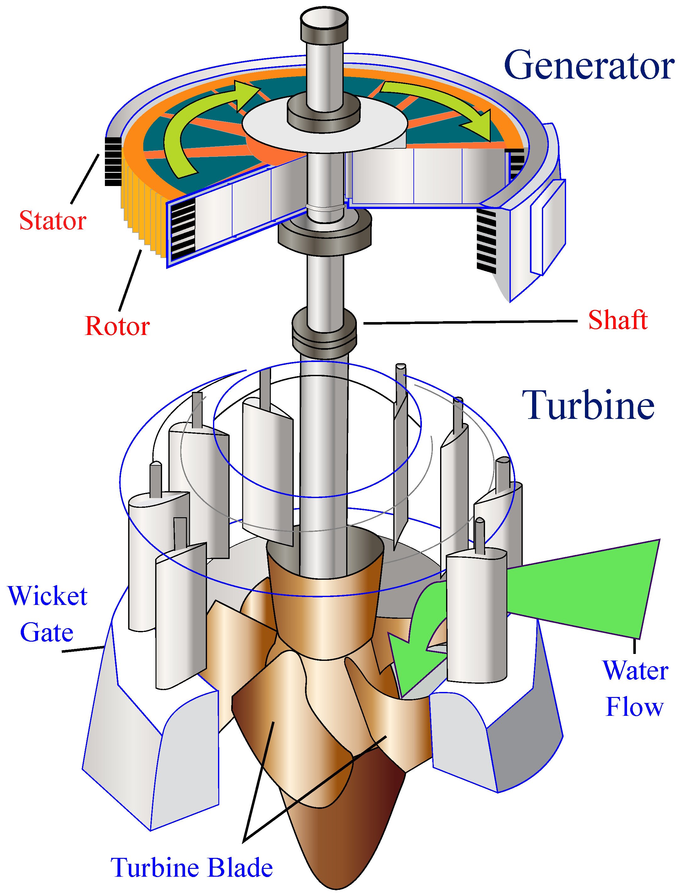
The power generated by a hydroturbine is influenced by its efficiency, head, and flow rate. For the Kaplan hydroturbine, when the water head is low and the length of the penstock is short, the water flow is nonelastic. Double-regulated turbines such as Kaplan and Bulb turbines are commonly used for low-head applications. Kaplan turbines are equipped with a propeller-type runner featuring adjustable blades that can rotate to change the water’s angle of attack as shown in Figure 1. This configuration allows the turbine to maintain high efficiency over a wide range of head and flow conditions. Their operation relies on coordinated control of both the wicket gates and runner blade angles to effectively regulate the water flow into the turbine. [13].

Figure 1.
Hydraulic turbine and electrical generator. Adapted from [14] and modified.
2.1. Dynamic Model of Kaplan Hydroturbine
The water system of a Kaplan turbine includes a reservoir, penstock, turbine chamber, and discharge (tail water stream). The outputs of the water flow rate and turbine torque can be described by the following equations:
where H is the operating water height, is the turbine shaft speed, u is the inlet valve opening, and is the blade angle. Additionally, g and f are the nonlinear functions for the flow rate and turbine torque, respectively. Assuming the turbine operates at an operating point and considering the nonelastic water flow, we can introduce the relative (normalized) incremental values as follows:
where all variables are normalized incremental values: x for shaft speed, h for water head, q for water flow rate, for guide vane opening, and for blade angle. The nonlinear dynamics of the Kaplan hydroturbine can be linearized as a Francis hydroturbine, considering the blade angle to yield the following dynamic models for the driving torque and water flow in terms of the eight parameters as in [6]:
The Kaplan turbine has its particularity as blade angle adjustment is critical for optimal efficiency. These turbines operate under a wide range of flow conditions by maintaining optimal blade angles between the water flow and the blade surfaces. Thus, the blade angle, , is a function of the wicket gate opening, u, and the influence of water head, H, represented as:
which is normally approximated by a 5th order polynomial, this leads to the following linearized model:
By incorporating this relationship between the and , the expressions in (4) and (5) can be simplified to a six-parameter model:
Similarly, the flow rate can be expressed as
The coefficients and are derived by linearizing the original nonlinear equations around the operating point O. These coefficients depend on partial derivatives of the functions f (related to torque) and g (related to flow), evaluated at the operating point. Specifically, the coefficients are:
2.2. Simplified Hydroturbine Dynamic Model
The turbine shaft dynamics and water dynamics can be represented by the following simplified equations:
where represents the mechanical torque produced by the interaction of water flow within the hydroturbine, and is the load torque. The dynamic relationship of torque and power is given as:
where P is the power generated, is the incremental normalized turbine shaft speed, is the incremental normalized turbine guide valve opening, and is the incremental normalized water head. is a function governed by the six coefficients to be estimated. Expanding (11), we get:
where the unknown parameters to be estimated are .
The objective is to use the real plant data on the gate opening and power generated to estimate the above six coefficients so that the modeled power can be made as close as possible to the real power data when the model is subjected to the same input of the gate opening dataset. It is important to clarify that while the governing equation for developed torque includes the variables shaft speed x, gate opening u, and net head h, only the gate opening was available from measurements and used as an external input to the model. While the measurement for the only state variable was available but was not available in the plant dataset, it were internally estimated by solving the system of nonlinear differential Equations (10). These internal states were then used to compute the instantaneous power output. This structure enables the model to simulate system dynamics and reproduce power output even when internal state measurements are unavailable. This is then an optimization problem where the decision variables are the six coefficients grouped by and the objective function would be related to the error between the modeled power and the actual power. In the next section, such an optimization problem will be formulated together with the relevant optimization algorithm.
3. Optimization Problem Formulation
The cost function can be formulated by considering the sum of power square error (14) from the measurement and the simulation. Moreover, to account for the worst-case deviations across all time steps, the cost function also accounts for the maximum absolute error (15), avoiding the large peak errors and the rate of change of error (16) to penalize the large changes in the error. Therefore, the total cost function is then formulated as:
where are the weights given to reflect the relative importance of the error metrics. The power error terms in the above equation are given by
which is the quadratic error term between the modelled power and the actual power.
is the peak error term reflecting the maximum error between the modelled power and the actual power.
where it has been denoted that
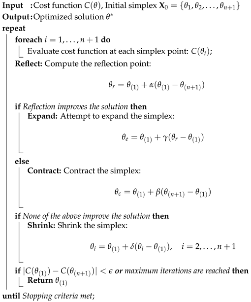
To estimate the parameters , the optimization problem is formatted using the Nelder–Mead Algorithm 1. This is a gradient-free optimization method designed to minimize objective functions in n-dimensional space. It works by iteratively refining the solution through evaluation of the objective function at several points and applying geometric transformations on a simplex consisting of points. This algorithm is particularly effective for solving optimization problems that do not rely on gradient information, making it ideal for non-differentiable, noisy, or complex objective functions. The optimization problem is formulated as:
The optimization problem seeks to minimize the cost function , where is the parameter vector to be estimated. The Nelder–Mead algorithm iteratively updates by reflecting, expanding, contracting, or shrinking a simplex of candidate solutions until convergence criteria are met.
| Algorithm 1: Nelder-Mead optimization algorithm. |
 |
In this work, the weights were intentionally set to unequal values and were chosen based on empirical evaluation to prioritize the overall match between simulated and measured power, while still penalizing significant transient errors and capturing dynamic mismatches. The selected weights were held constant throughout all experiments for consistency and are summarized in Table 1.

Table 1.
Summary of the system parameters and simulation settings.
4. Performance Metrics
Evaluation metrics are used to quantify the performance of the proposed model [15]. To evaluate the model’s performance, the agreement between simulated () and measured () power outputs was quantified using the following metrics:
4.1. Root Mean Squared Error (RMSE)
Measures the average magnitude of the errors. Lower values indicate better fit. n is the number of data points.
4.2. RMSE Percentage
A relative error metric, normalizing RMSE by the mean of measured values (). Lower values indicate a relatively better fit.
where .
4.3. Coefficient of Determination ()
The coefficient of determination, , measures how well the model explains the variability in the observed data. It ranges from 0 to 1, with values closer to 1 indicating a better fit.
where is the sum of squared residuals and is the total sum of squares.
4.4. Adjusted
Adjusts based on the number of parameters (p) and data points (n), penalizing model complexity. Useful for comparing models. Higher values are preferred.
4.5. F-Statistic
Tests the overall statistical significance of the model’s fit, assessing if it explains variance better than the mean. Larger values suggest higher significance.
where sum of squares of regression .
5. Simulation Setup and Results
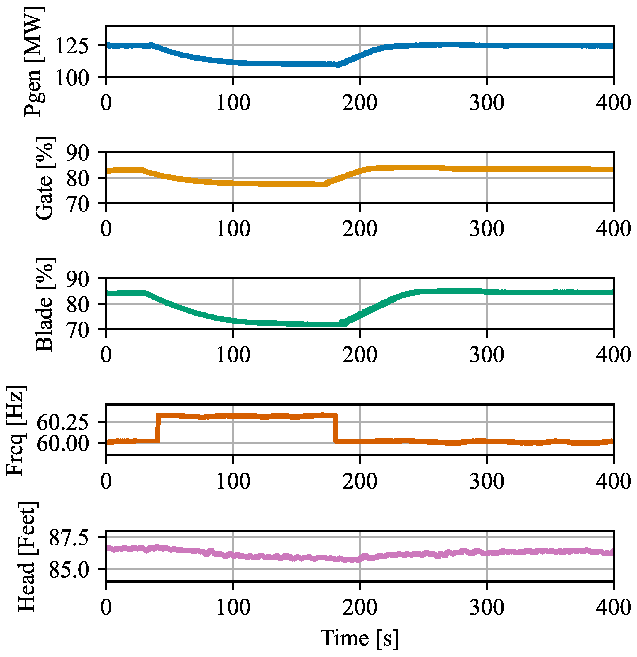
The real operational data are taken from Unit C-8 at the Rocky Reach Dam, owned and operated by Chelan County Public Utility District (PUD), Washington. The operational data were collected to accurately model the dynamic performance of the hydroelectric system, including the turbine dynamics, in accordance with the North American Electric Reliability Corporation. The experimental dataset used for parameter identification spans a total duration of 400 s and contains 1492 data points per measured variable (gate opening, net head, and generated power) and the collected data are shown in Figure 2. Considering the inherently slow dynamics of hydro turbines, this resolution is sufficient to capture the relevant transient and steady-state behavior of the system for parameter identification and model validation. Notably, the gate opening data used in this study represent the real plant control input over the measurement period and exhibits a change of approximately +0.3, p.u. during the event window, which corresponds to typical turbine operating conditions and load demands. These variations capture the dynamic response of the turbine and provide the excitation needed for system identification and parameter optimization. The temporal profile of the gate opening, illustrated in Figure 2, highlights periods of steady operation as well as transient changes, which are essential for validating the dynamic model against plant data.
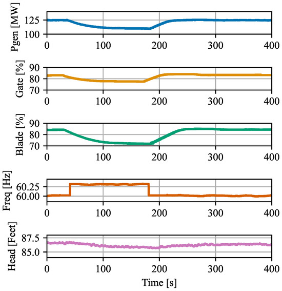
Figure 2.
Measurements for the unit response to a +0.3 Hz step from the Kaplan hydroturbine from the Rocky Reach Dam.
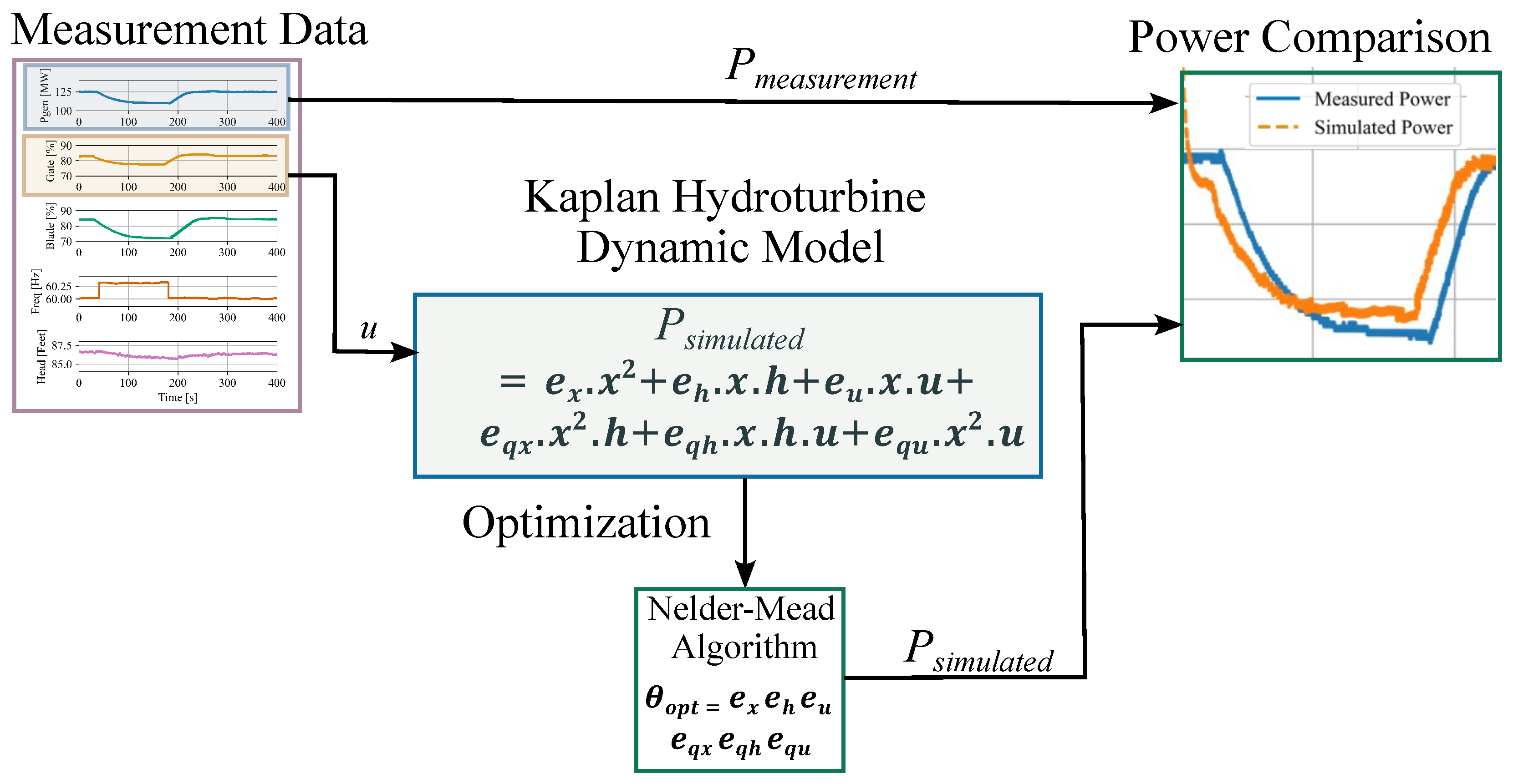
Figure 3 shows the simulation setup for the formulation of the optimization problem. The goal is to tune the Kaplan hydroturbine model using the operational data from the Rocky Reach Dam to match the mechanical power output from the plant with the simulated model by optimizing the Kaplan model’s six coefficients. The weights are selected based on the relative importance of each error metric. Table 1 summarizes the system parameters and simulation settings for this optimization problem formulation. On note, the error tolerance is adaptive throughout the simulation.
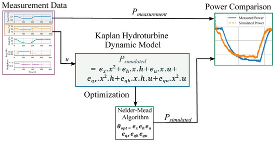
Figure 3.
Simulation setup showing the Nelder–Mead algorithm-based optimization of coefficients of the Kaplan hydroturbine dynamic model based on the inlet gate value opening to the turbine.
The guide vane opening of the hydroturbine system serves as the model’s time-varying control input. To facilitate open-loop simulations, the data are interpolated to align with the solver’s time steps, providing a continuous representation of the gate opening over time. The simplified dynamic model incorporating the relationship of the blade angle and the gate value opening is used as stated in Equation (11). Figure 2 shows the data collected from the Chelan County PUD’s Rocky Reach Dam, Unit C-8, under Hz online perceived frequency step test. For the optimization problem, only the gate (%) was used as an input to the dynamic model to estimate the six unknown coefficients so that the simulation’s mechanical power output matches the measurement ().
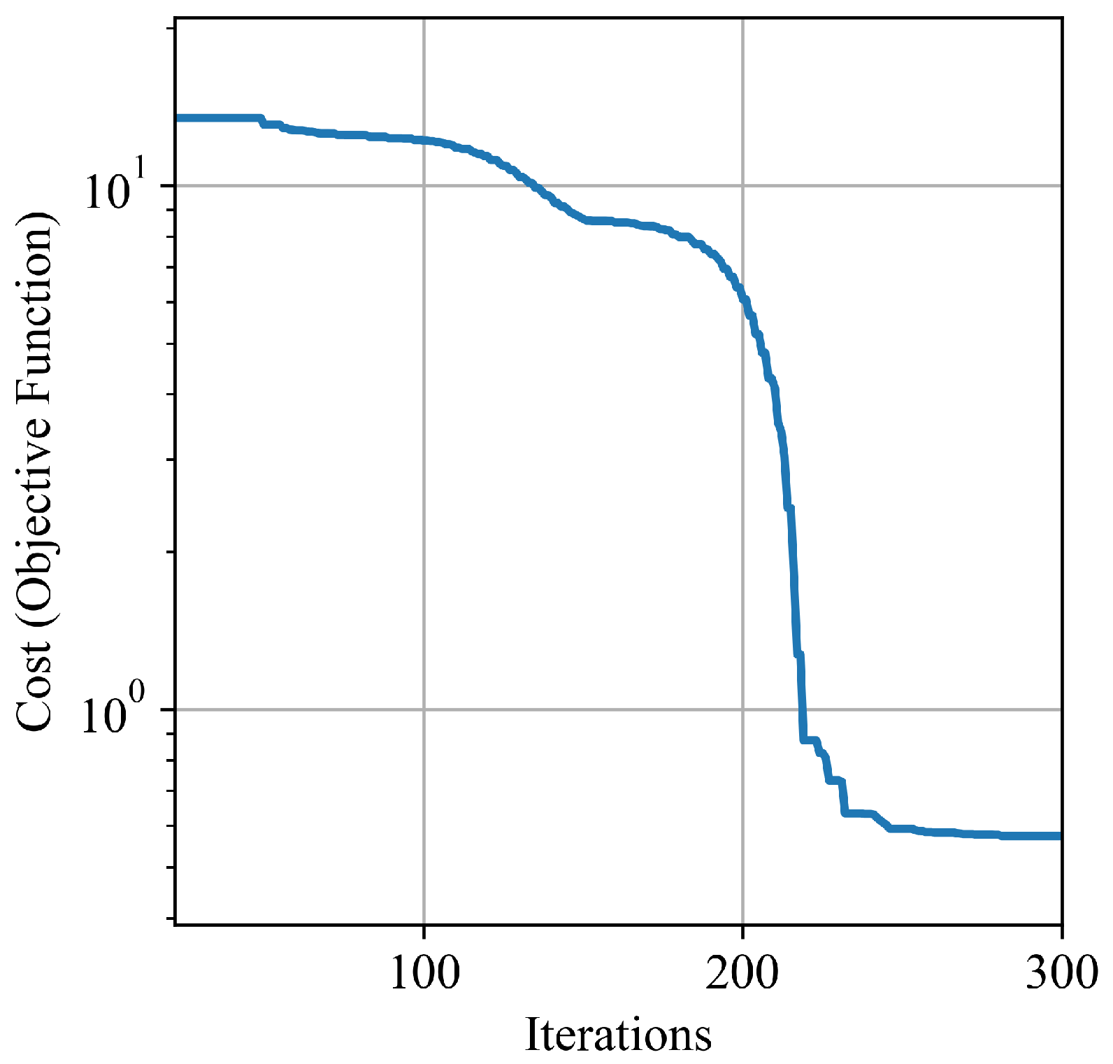
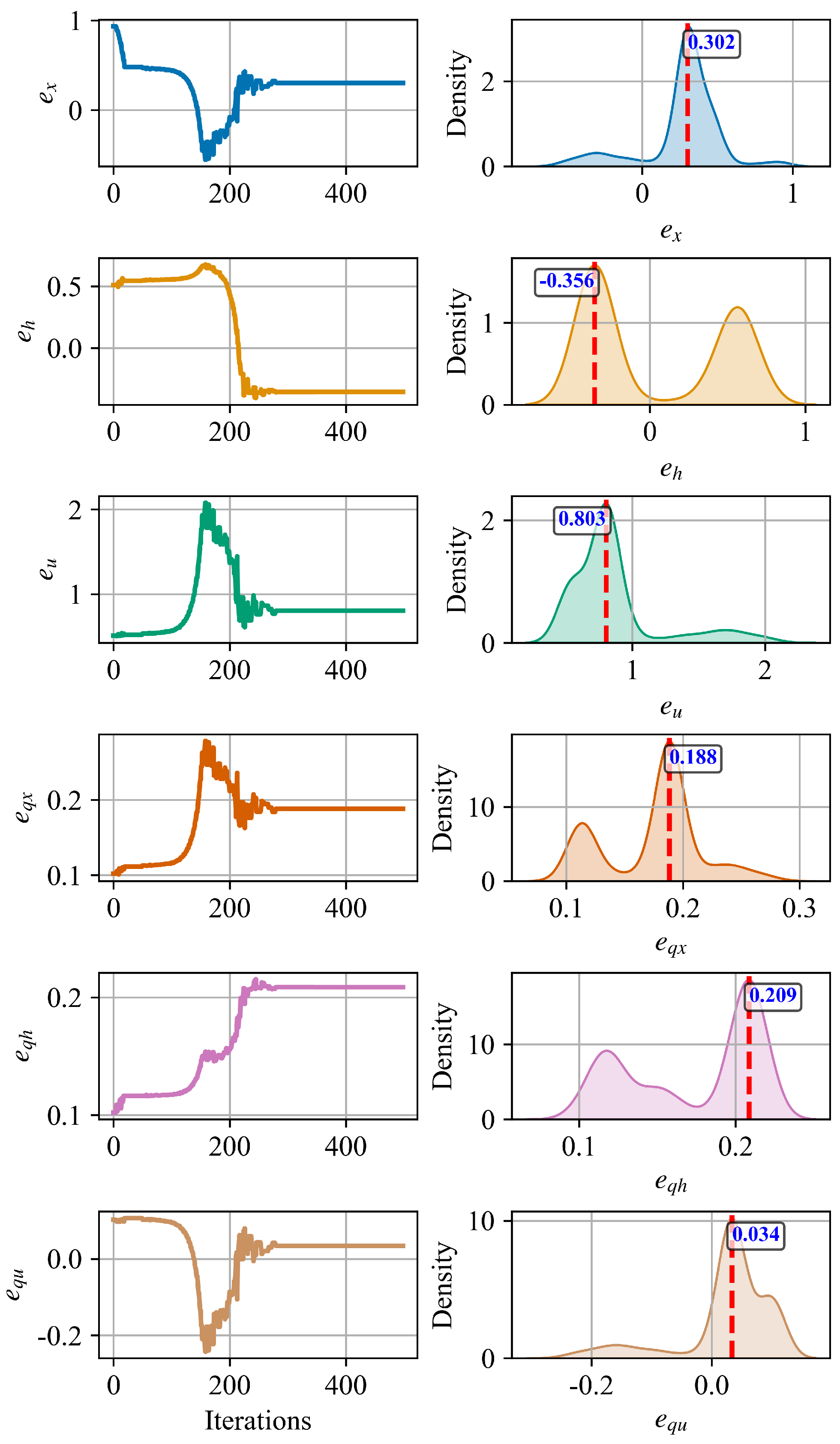
The convergence performance of the Nelder–Mead optimization on minimizing the cost function over the number of iterations is shown in Figure 4. With the optimization problem formulation, the convergence and distribution of the estimated best six coefficients of the Kaplan hydroturbine model that represent the real Kaplan unit in Rocky Reach Dam are shown in Figure 5. The model was simulated with the initial parameters listed in Table 1. Results show that the parameters converged after around 200 iterations. The final estimated coefficients’ values are annotated in the probability density function plot and yielded the following estimated parameters for the model, represented by the vector . Estimated coefficients reflect the contribution of different terms in the governing equations to the simulated power output. Notably, parameters such as and exhibit higher values, indicating a stronger influence of the corresponding terms on the model’s response. In contrast, coefficients like have smaller magnitudes, suggesting a relatively lower impact. This variation highlights which physical relationships are more dominant in the power estimation process. Such information is valuable for model refinement, allowing future efforts to prioritize or simplify certain terms based on their relevance to the overall system dynamics.
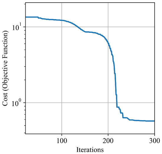
Figure 4.
Convergence performance of the cost function over the iterations.
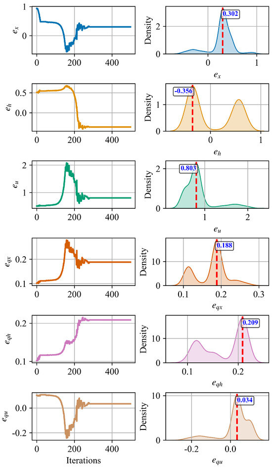
Figure 5.
The six estimated coefficients’ convergence and the probability density function of the estimated coefficients for the Kaplan hydroturbine model.
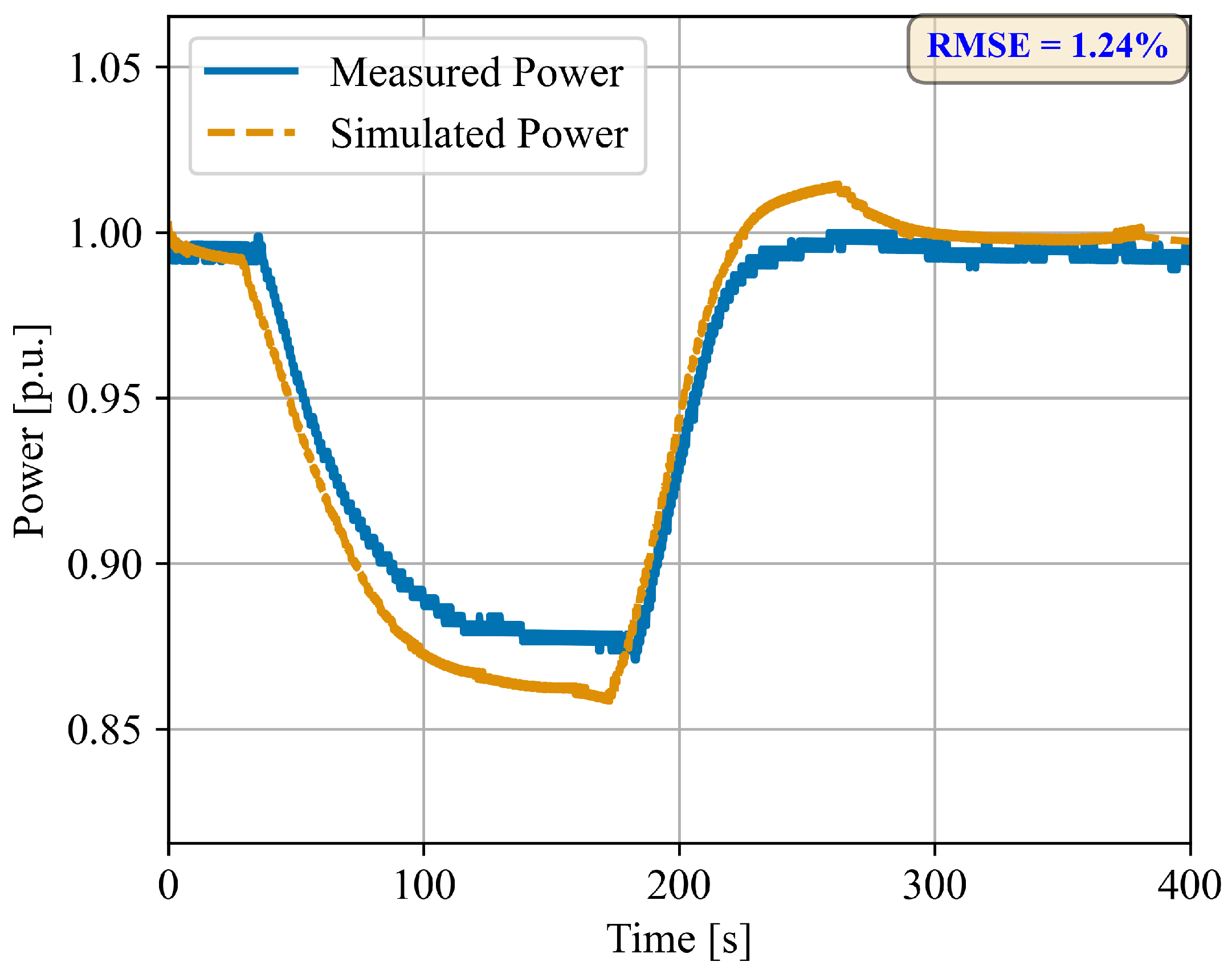
Estimated mechanical power output from the simulated model with optimized parameters is shown in Figure 6. The formulated optimization problem can closely predict the mechanical power output from the real Kaplan hydroturbine unit based on the single gate vane opening as an input while optimizing the coefficients of the developed model. Since parameters can be estimated for given operating condition, these parameters can be used to estimate the power output from the Kaplan hydropower online with given gate-opening as input. Model performance was evaluated using key statistical metrics comparing the simulated power output to the measured plant data and summarized in Table 2. An RMSE of 0.0118, corresponding to an RMSE percentage of 1.24%, indicates a very low average and relative error, demonstrating excellent accuracy in capturing the measured power profile. The coefficient of determination, , was 0.9425, signifying that the model explains over 94% of the variance in the measured data, indicating a strong fit. The adjusted of 0.9422, being very close to R2, further supports that the chosen parameters are effective and the model complexity is appropriate. The large F-statistic of 5910.3983 confirms the high statistical significance of the model’s fit.
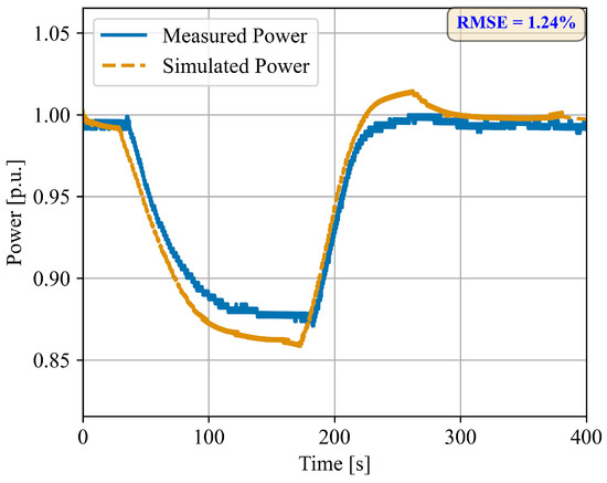
Figure 6.
Estimated Kaplan hydroturbine mechanical power output from the simulation compared with the measured mechanical power output of the Rocky Reach Dam unit.
Table 2.
Model performance metrics with fewer datasets.
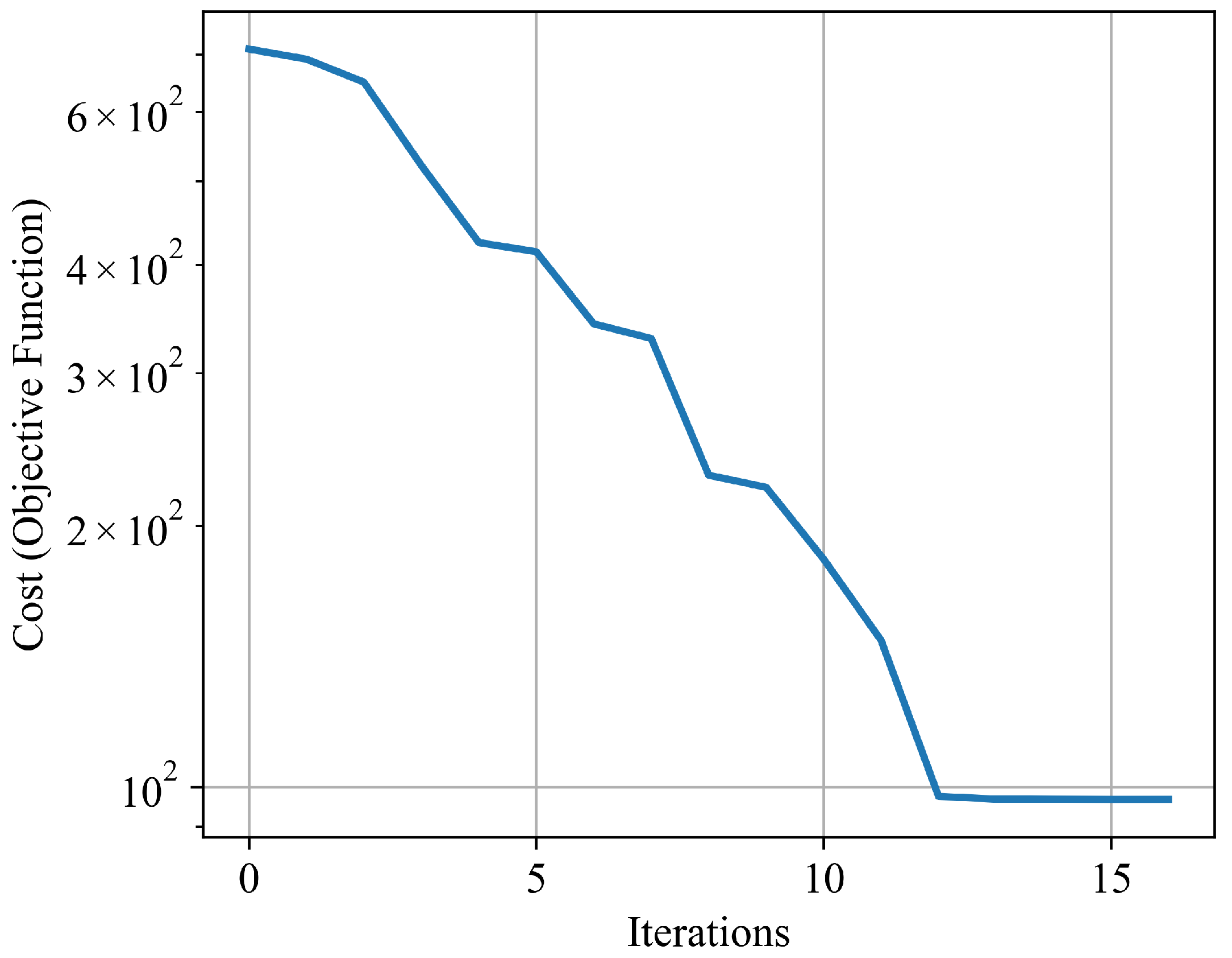
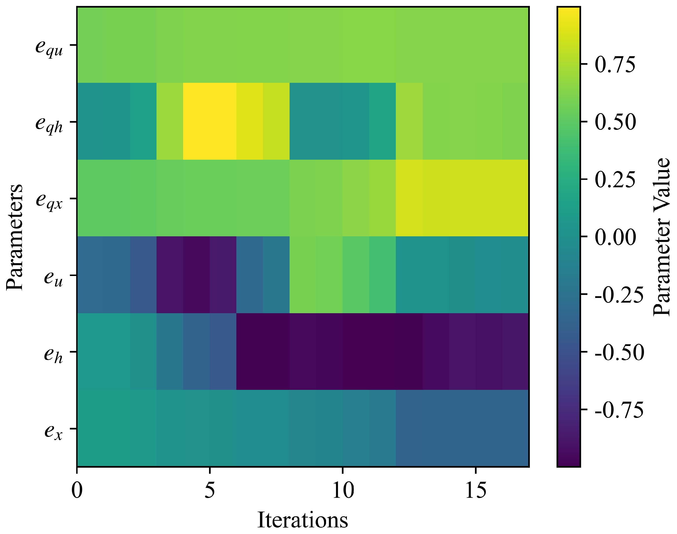
The algorithm is then tested with a dataset covering a longer period. Seven days of data from April 2024 are taken for the validation. The cost function of the optimization is shown in Figure 7. The optimization process yielded the following estimated parameters for the model, represented by the vector : as shown in Figure 8.
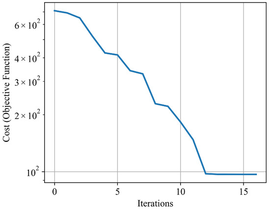
Figure 7.
Convergence performance of the cost function over the iterations.
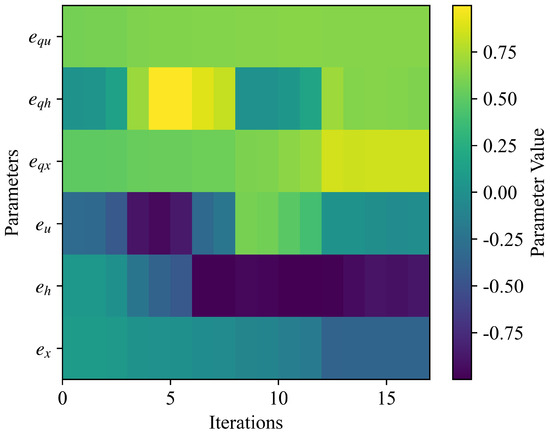
Figure 8.
Heat map representing the estimated six coefficients of the Kaplan hydroturbine model.
To validate the model under a broader range of operating conditions, we utilized an extended dataset comprising seven consecutive days of real operational data from the plant. The model’s performance over this longer time horizon was evaluated using key statistical metrics, as summarized in Table 3. Figure 9 shows the performance of the proposed model with validation data. The RMSE was 0.0394, with an RMSE percentage of 4.93%, indicating low absolute and relative error between the simulated and measured power outputs. The coefficient of determination () was 0.9248, demonstrating that the model explains approximately 92.48% of the variance in the measured data—reflecting a strong fit. The adjusted , also 0.9248, suggests that the model complexity is well-suited to the dataset and the selected parameters are effective. Additionally, the high F-statistic value of 161,921.7939 confirms the model’s strong statistical significance. These results collectively highlight the model’s robustness and reliability when validated against a longer and more diverse dataset.
Table 3.
Model performance metrics with the longer dataset.
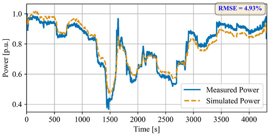
Figure 9.
Estimated Kaplan hydroturbine mechanical power output from the 7-day-long simulation compared with the measured mechanical power output of the Rocky Reach Dam unit.
Accurately modeling the complex nonlinear dynamics inherent in a Kaplan hydroturbine, particularly the relationship between gate opening and power output, presents a significant challenge. The adopted linearized model simplifies these dynamics effectively around an operating point for analytical purposes. Validation of this model using the current available dataset of real plant operational data has demonstrated good performance, evidenced by the high and low RMSE values achieved.
6. Conclusions
This paper first derives a six-coefficient linearized dynamic model for a Kaplan hydroturbine. An optimization problem is then formulated to estimate these six unknown coefficients by minimizing the error between the model’s mechanical power output and real plant data, using the gate vane opening as input. The approach is demonstrated using real field data from the Rocky Reach Dam Unit C-8, comparing the plant’s power output with the simulated power from the optimized model. Validation with this dataset shows that the proposed optimized linearized model achieves good performance and can capture the dominant turbine dynamics under the tested conditions. Considering the given data, even this linearized optimization-based model demonstrates a strong capability to capture dynamics, providing optimal parameter tuning beneficial for controller design and maintenance. To further enhance the model’s accuracy and robustness, testing will be conducted as new data become available, and exploration of nonlinear modeling approaches will be pursued for broader applicability. Additionally, comparing the proposed optimization method with alternative techniques could offer further insights and improve overall solution robustness.
Author Contributions
Conceptualization, H.W.; methodology, H.W. and S.S.; software, S.S.; validation, H.W. and S.S.; formal analysis, S.S.; investigation, S.S.; resources, W.J.; data curation, W.J.; writing—original draft preparation, H.W. and S.S.; writing—review and editing, H.W., S.S., and W.J.; visualization, S.S.; supervision, H.W.; project administration, H.W.; funding acquisition, H.W. All authors have read and agreed to the published version of the manuscript.
Funding
This work was supported in part by UT–Battelle LLC, through the US Department of Energy (DOE) under contract DE-AC05-00OR22725, and in part by the DOE Water Power Technologies Office under the Development of a Digital Twin for Hydropower Systems.
Institutional Review Board Statement
Not applicable.
Data Availability Statement
Data are unavailable due to privacy restrictions.
Acknowledgments
This manuscript has been authored in part by UT-Battelle LLC under Contract DE-AC05-00OR22725 with the US Department of Energy (DOE). The US government retains and the publisher, by accepting the article for publication, acknowledges that the US government retains a nonexclusive, paid-up, irrevocable, worldwide license to publish or reproduce the published form of this manuscript, or allow others to do so, for US government purposes. DOE will provide public access to these results of federally sponsored research in accordance with the DOE Public Access Plan (http://energy.gov/downloads/doe-public-accessplan, accessed on 1 January 2020). The authors have reviewed and edited the output and take full responsibility for the content of this publication.
Conflicts of Interest
Author Wenbo Jia was employed by Chelan County PUD. The remaining authors declare that the research was conducted in the absence of any commercial or financial relationships that could be construed as a potential conflict of interest.
Abbreviations
The following abbreviations are used in this manuscript:
| Linearized coefficients for turbine torque: turbine speed, water pressure, guide vane opening | |
| Linearized coefficients for water flow rate: turbine speed, water pressure, guide vane opening | |
| h | Normalized incremental water head |
| u | Guide valve opening (time-variant) |
| x | Normalized incremental turbine shaft speed |
| q | Normalized incremental water flow rate |
| Blade angle | |
| m | Load torque |
| H | Operating water height |
| Turbine shaft speed | |
| g | Nonlinear functions for flow rate |
| f | Nonlinear functions for turbine torque |
| O | Operating point |
| Water inertia time constant | |
| J | Equivalent inertia |
| M | Turbine torque |
| Q | Water flow rate |
| Turbine operating torque at operating point | |
| Public Utility District | |
| Root mean square error | |
| Coefficient of determination |
References
- Akinyemi, O.S.; Chambers, T.L.; Liu, Y. Evaluation of the power generation capacity of hydrokinetic generator device using computational analysis and hydrodynamic similitude. J. Power Energy Eng. 2015, 3, 71. [Google Scholar] [CrossRef]
- Uría-Martínez, R.; Johnson, M.M. U.S. Hydropower Market Report, 2023rd ed.; Oak Ridge National Laboratory: Oak Ridge, TN, USA, 2023.
- Rauniyar, M.; Berg, S.; Subedi, S.; Hansen, T.M.; Fourney, R.; Tonkoski, R.; Tamrakar, U. Evaluation of probing signals for implementing moving horizon inertia estimation in microgrids. In Proceedings of the 2020 52nd North American Power Symposium (NAPS), Tempe, AZ, USA, 11–13 April 2021; IEEE: Tempe, AZ, USA, 2021; pp. 1–6. [Google Scholar]
- Fang, H.; Chen, L.; Dlakavu, N.; Shen, Z. Basic modeling and simulation tool for analysis of hydraulic transients in hydroelectric power plants. IEEE Trans. Energy Convers. 2008, 23, 834–841. [Google Scholar] [CrossRef]
- Rios, L.M.; Sahinidis, N.V. Derivative-free optimization: A review of algorithms and comparison of software implementations. J. Glob. Optim. 2013, 56, 1247–1293. [Google Scholar] [CrossRef]
- Wang, H.; Yin, Z.; Jiang, Z.-P. Real-time Hybrid Modeling of Francis Hydroturbine Dynamics via a Neural Controlled Differential Equation Approach. IEEE Access 2023, 11, 139133–139146. [Google Scholar] [CrossRef]
- Masood, Z.; Khan, S.; Qian, L. Machine learning-based surrogate model for accelerating simulation-driven optimisation of hydropower Kaplan turbine. Renew. Energy 2021, 173, 827–848. [Google Scholar] [CrossRef]
- Chamil, A. Modelling and optimisation of a Kaplan turbine—A comprehensive theoretical and CFD study. Clean Energy Syst. 2022, 3, 100017. [Google Scholar]
- Dahlborg, E.; Norrlund, P.; Saarinen, L. Kaplan turbine model validation for large grid frequency disturbances. IEEE Trans. Energy Convers. 2020, 36, 611–618. [Google Scholar] [CrossRef]
- Brezovec, M.; Kuzle, I.; Tomisa, T. Nonlinear digital simulation model of hydroelectric power unit with Kaplan turbine. IEEE Trans. Energy Convers. 2006, 21, 235–241. [Google Scholar] [CrossRef]
- Menarin, H.A.; Costa, H.A.; Fredo, G.L.M.; Gosmann, R.P.; Finardi, E.C.; Weiss, L.A. Dynamic modeling of Kaplan turbines including flow rate and efficiency static characteristics. IEEE Trans. Power Syst. 2019, 34, 3026–3034. [Google Scholar] [CrossRef]
- Pan, H.; Dou, Z.; Cai, Y.; Li, W.; Lei, X.; Han, D. Digital twin and its application in power system. In Proceedings of the 2020 5th International Conference on Power and Renewable Energy (ICPRE), Shanghai, China, 26–29 September 2020; pp. 21–26. [Google Scholar]
- Dobrijevic, D.M.; Jankovic, M.V. An improved method of damping of generator oscillations. IEEE Trans. Energy Convers. 1999, 14, 1624–1629. [Google Scholar] [CrossRef]
- Water Turbine. Available online: https://simple.wikipedia.org/wiki/Water_turbine (accessed on 9 April 2025).
- Dou, Y.; Ricks, T.M.; DuBien, J.L.; Lacy, T.E., Jr.; Liu, Y. Response surface modeling to facilitate the parametric study of transversely impacted pressurized pipelines. Thin-Walled Struct. 2017, 119, 646–652. [Google Scholar] [CrossRef]

Disclaimer/Publisher’s Note: The statements, opinions and data contained in all publications are solely those of the individual author(s) and contributor(s) and not of MDPI and/or the editor(s). MDPI and/or the editor(s) disclaim responsibility for any injury to people or property resulting from any ideas, methods, instructions or products referred to in the content. |
© 2025 by the authors. Licensee MDPI, Basel, Switzerland. This article is an open access article distributed under the terms and conditions of the Creative Commons Attribution (CC BY) license (https://creativecommons.org/licenses/by/4.0/).