Abstract
This research work aims to design and develop a dynamic vibration absorber that effectively reduces the vibrations of a flexible structure subjected to external loads. The analysis presented in this paper initially focuses on identifying the resonance frequencies of a typical structural system, which serves as the case study, since these frequencies are critical to dampening due to their potential to cause excessively large vibration amplitudes. Following this, the optimal parameters of the vibration absorber, including the mass, stiffness, and damping characteristics of the proposed design, were determined. Additionally, this paper proposes and examines the use of viscous-type damping, which is achieved through piston–cylinder systems connected to the structural components of the analyzed frame structure. Thus, the main contributions of this work include the analytical dimensioning, the technical design, and the virtual prototyping of a dynamic absorber constructed using a guyed mast structure capable of significantly reducing mechanical vibrations. This design solution ultimately enhances the strength and durability of the frame structure represented in the case study under external excitation, particularly in the worst-case scenario of seismic action. Furthermore, a key aspect of this study is implementing a new numerical procedure for identifying the system equivalent stiffness coefficient based on its mass and modal parameters, which is particularly useful in engineering applications. The numerical experiments conducted in this work support the effectiveness of the proposed design solution, devised specifically for the dynamic vibration absorber developed in this paper.
1. Introduction
1.1. Background Information and Research Significance
This section provides background material that introduces the issues addressed in this investigation. First, it highlights the significance of the current research, clarifying the specific research questions to be examined and resolved in this study. Next, a brief literature review is included to help readers who may be unfamiliar with some of the topics discussed in this paper. Following that, the scope of this paper is summarized, along with the contributions made in this investigation. Lastly, the structure of the manuscript is outlined to present the content of the entire paper.
The control of structural vibrations in the mechanical, aerospace, transportation, and civil fields has become increasingly important in recent years [1,2,3]. A fundamental challenge in designing civil and industrial structures is the high levels of vibratory stress they encounter due to environmental factors, such as strong winds or heightened sensitivity to seismic activity in the areas where the structures are located [4]. Within the field of existing structure rehabilitation, design methods based on dynamic vibration absorbers can represent a less invasive alternative to approaches involving structural strengthening with either steel or fiber-reinforced plastic (FRP) materials [5,6,7]. Vibrational stresses can also originate from human and mechanical sources, such as groups of people rapidly moving up and down a staircase or large crowds walking together. This can lead to significant problems in large structures, such as stages, if they lack adequate vibration-damping systems [8]. In industrial and manufacturing engineering, vibrations from heavy machinery, generators, and diesel engines also pose a threat to structural integrity, particularly when these are installed on steel frameworks or floors [9]. In marine engineering, large cruise ships can employ tuned mass dampers to protect the vessel structure from vibrations created by the engine [10].
To address the potentially harmful vibration issues mentioned earlier, particular attention is focused on non-dissipative systems known as dynamic absorbers, which alter the behavior of buildings in seismic regions or areas with high winds. These devices, more specifically referred to as tuned vibration absorbers (TVAs), are utilized for vibration control in mechanical systems and, since their invention by Frahm, who patented it in 1911 [11], have been the subject of numerous studies and have been successfully applied to resolve real-world problems [12,13]. The purpose of these devices is to absorb a portion of the incoming mechanical energy, thereby reducing the energy demand on the structure and minimizing the potential for damage. Further studies on these systems have encouraged the widespread use of tuned mass dampers, particularly in civil engineering. An example is the Citigroup Center in New York, designed by William LeMessurier in the mid-twentieth century and completed in 1977. It was one of the first skyscrapers to employ a tuned mass damper to reduce oscillations. Another example is the Taipei 101 skyscraper in Taiwan, which contains the largest tuned mass damper in the world.
Passive control is the most established technology, originating in the 1910s when Frahm received a U.S. patent for the dynamic vibration absorber (DVA) [11]. Numerous articles on earthquake-passive structural control have been published recently. One of the first applications of TMDs was in the 244 m, 60-story John Hancock building in Boston in 1977 to mitigate wind vibration responses [14]. It features two 300-ton TMDs, each consisting of a 5.2 × 5.2 square and a 1 m deep lead-filled steel box mounted on a 9 m long steel plate. They are positioned at either end of the 58th floor, 67 apart, and are tuned to a vibration frequency of 0.13 , which corresponds to the estimated fundamental frequency of the structure. Other recent examples include the Citicorp Building in New York City, the 101-story Taipei 101 in Taipei, the Aspire Tower in Doha, Qatar, and the Shanghai World Financial Center in Shanghai, China.
To conclude, the examples discussed above demonstrate the importance of structural vibration control in various mechanical engineering applications.
1.2. Formulation of the Research Question to Be Addressed in This Investigation
In recent years, structural health monitoring and vibration control have become crucial issues in mechanical, aerospace, and civil engineering, particularly in designing buildings and infrastructure exposed to environmental stresses such as strong winds and seismic events. The term “Vibration Control” refers to a collection of techniques and devices that facilitate the rapid, reliable, and precise mitigation of vibrations in machines and structures caused by both their operation and external stresses. Vibrations in a structure may arise from natural forces such as wind or earthquakes, or from seemingly benign sources that produce destructive reverberations within the structure. For instance, seismic waves generate oscillations throughout the height of structures [15,16]. As a result, seismic motion can lead to significant movements in buildings, while wind pressure against tall structures can cause notable shifts at the tops of skyscrapers, reaching up to a meter [17,18]. These concepts are fundamental to modern anti-seismic regulations, under which most buildings are designed to endure considerable damage during exceptional events like earthquakes while avoiding collapse to protect human lives [19,20]. While damage allows for the dissipation of a large portion of the input energy, the resulting permanent deformations necessitate substantial and costly recovery (or even demolition and reconstruction), leaving the structure more vulnerable to future events. In addition to the necessity of preserving human lives, this alternative design philosophy also takes into account other requirements, such as minimizing structural damage [21].
One possible way to apply the principles discussed earlier is by using the techniques of the structural control concept, which Yao first formalized in 1972 and applies theories of automatic controls to civil engineering [22]. Recently, structural control methods, such as those presented in [23], have gained popularity because they can design structures capable of withstanding large-scale dynamic actions [24,25]. While minimizing the response amplitude is important, simplicity, reliability, and energy efficiency are also essential in civil engineering. Today, it is necessary to study reliable protection systems for structures that can effectively withstand seismic and wind forces. Various vibration control equipment can be used to establish a suitable configuration to enhance structural performance.
Generally, four different approaches can be used to control vibrations in flexible structures: passive control, active control, semi-active control, and hybrid control. Synthetically, passive systems do not require any external energy to function. They rely on materials and devices that absorb and dissipate energy, such as tuned mass dampers (TMDs), base isolators, and viscoelastic dampers. Mechanically, these systems are typically simpler and more reliable because they have fewer moving parts. Active systems, on the other hand, use external energy sources to actively counteract externally induced vibrations. They employ sensors and actuators to monitor and adjust the structural response in real-time, providing enhanced performance compared to passive systems. However, active systems tend to be more complex and costly. Semi-active systems, positioned halfway between the active and passive control approaches, combine features of both systems, using external power to adjust passive devices. They can change their damping characteristics in response to vibrations, offering a balance between performance and energy efficiency. Examples of semi-active systems include magnetorheological dampers and semi-active tuned mass dampers. Hybrid systems integrate both passive and active control methods to maximize the benefits of both systems, providing robust and efficient vibration control. Although hybrid systems are more complex, they can offer the best overall performance for vibration control.
This paper focuses on developing a simple dynamic vibration absorber for a laboratory test rig and, more specifically, on creating viable design solutions that convert the analytical values of the physical parameters derived from the theory of mechanical vibrations into practical mechanical components that are readily available off the shelf for assembling a functioning mass damper.
1.3. Literature Review
As mentioned before, the vibration control of structures can be achieved through four innovative methods: passive, active, semi-active, and hybrid systems. Passive control employs systems that generate a control force in response to the motion of the structure through appropriate devices, which cannot be modified after installation without requiring external energy. Generally, methods for protecting structures include isolation, dissipation, additional energy supply, and the use of tuned mass dampers (TMDs). TMDs limit energy input and dissipate most of it in specialized devices [26,27]. Passive control technologies have long been integrated into civil applications and serve as an effective and reliable control tool [28,29]. Compared to other methods, their most significant disadvantage is their inability to adapt to actual operating conditions, such as unpredictable inputs and/or structural responses, since their design can only be based on anticipated excitation [30,31].
Active control (AC) systems utilize external actuators to apply control forces to a structure [32,33]. The magnitude of these forces is determined in real-time based on a predetermined control algorithm and is considered a function of the structural response and/or the excitation itself [34,35]. Active systems require a source of external energy and an integrated system for information collection (sensors), data processing (control units), and mechanisms capable of applying the control force on the structure (actuators) [36,37,38]. These systems, characterized by their adaptability to actual operating conditions, can yield excellent results, particularly in the aeronautical and aerospace engineering fields [39]. Design constraints, such as significant space limitations, may prevent using an active mass damper (AMD) system. This is exemplified by the active mass damper or active mass driver system designed and installed in the Kyobashi Seiwa Building in Tokyo and the Nanjing Communication Tower in Nanjing, China [40]. The Kyobashi Seiwa Building represents the first full-scale implementation of active control technology and consists of 11 stories with a total floor area of 423 [41,42]. The control system features two AMDs, with the primary AMD used for transverse motion, weighing four tons, while the secondary AMD weighs one ton and is employed to reduce torsional motion [43,44,45]. The active system aims to minimize building vibrations during strong winds and moderate earthquake excitation, enhancing occupant comfort.
Semi-active control (SA) is realized through the real-time regulation of the mechanical parameters of the control devices, which interact passively with the rest of the structure in response to structural motion. Adjusting these parameters is based on a selected control algorithm, according to the excitation and/or the structural response [46]. Therefore, similarly to AC, the system requires sensors, processors, and actuators. However, the external energy required is minimal compared to active systems, which is just enough to change the mechanical characteristics of the devices, and can be supplied, for example, by a simple battery [47,48,49]. These devices rely on the real-time modification of mechanical characteristics, which then interact passively with the structure and have minimal demands for external energy, potentially combining the reliability and simplicity of passive systems with the adaptability of active ones [50,51]. A semi-active shock absorber system was recently installed in the Kajima Shizuoka Building in Shizuoka, Japan. Semi-active hydraulic shock absorbers were installed within the walls on both sides of the building to allow its use as a rescue base in post-earthquake situations. Each damper contains a flow control valve, a check valve, and an accumulator, capable of developing a maximum damping force of 1000 [52]. Another class of semi-active devices uses controllable fluids. Compared to previous semi-active damper systems, an advantage of controllable fluid devices is that they do not contain moving parts other than the piston, making them potentially very reliable.
The essential characteristics of controllable fluids lie in their ability to reversibly change from a fluid with free, viscous, and linear flow to a semi-solid with yield strength in milliseconds when exposed to an electric field for electrorheological (ER) fluids or a magnetic field for magnetorheological (MR) fluids [53]. In the case of MR fluids, they typically consist of magnetically adjustable micron-sized particles dispersed in a carrier medium such as mineral or silicone oil. When a magnetic field is applied to the fluid, chains of particles form, and the fluid becomes semi-solid, exhibiting viscoplastic behavior. The transition to rheological balance can be achieved in a few milliseconds, enabling the construction of devices with high bandwidth. Effectively, MR fluids can operate at temperatures ranging from 7.4 °C to 150.8 °C, with only slight variations in yield stress. They are not sensitive to impurities commonly encountered during production and operation, and the separation of small fluid particles occurs under typical flow conditions.
Furthermore, a wider range of additives (surfactants, dispersants, friction modifiers, anti-wear agents, etc.) can generally be employed with MR fluids to enhance stability, seal life, bearing life, etc., as electrochemistry does not impact the magnetopolarization mechanism. Additionally, MR fluid can be easily controlled with low voltage (e.g., 12–24 ) output from the power supply, driven by a current of 1 ± 2 . While there are currently no applications for large-scale structural MR devices, their future in civil engineering applications appears promising. Reports have been published on the design of a 20-ton, life-size MR shock absorber, demonstrating that this technology is scalable for suitable civil engineering devices. In the design speed range, the dynamic forces generated by this device exceed 10 , yet the total power required by the device is only 20 ± 50 [54].
Hybrid control involves combining the systems described above. In these cases, a passive system acts with an active or semi-active system to improve performance. External energy demands are reduced by the presence of the passive system, which guarantees the minimum level of reliability. Applications of these systems include hybrid insulation for bridges or buildings, or, in general, hybrid mass dampers (HMDs). The HMD system is the most common control device in large-scale civil engineering applications. An example of this application is the HMD installed in the Sendagaya INTES building in Tokyo in 1991 [55]. The HMD was installed on top of the 11th floor and consists of two masses to control the transverse and torsional motions of the structure. At the same time, hydraulic actuators provide active control capability. Storage tanks for thermal ice are used as mass blocks so that there are no additional costs due to a possible new mass. The masses are supported by multistage rubber bearings designed to reduce the control energy consumed in HMD and ensure fluid mass movements. Data obtained to evaluate the system performance when subjected to strong winds on 29 March 1993 showed promising results. Variations in such HMD configurations include multi-step pendulum HMDs installed, for example, in the Yokohama Landmark Tower in Yokohama, the tallest building in Japan, and the TC Tower in Kaohsiung, Taiwan. Additionally, the HMD DUOX system, which consists of a TMD actively controlled by an auxiliary mass, was installed, for example, in the Ando Nishikicho building in Tokyo [56,57].
Dynamic vibration absorbers (DVAs), also known as vibration neutralizers (VNs) or tuned mass dampers (TMDs), are auxiliary systems comprising inertia, stiffness, and damping elements that, when connected to a given structure or machine, referred to herein as the primary system, can absorb vibratory energy at the connection point [58]. The family of TMDs is divided into four categories: conventional TMDs, pendulum TMDs (PTMDs) [59,60,61], bi-directional TMDs (BTMDs) [62], and tuned liquid column dampers (TLCDs) [63,64,65,66]. One of the first applications of TMD was the 244 m sixty-story John Hancock building in Boston in 1977 to reduce the response to wind vibrations [67,68]. Since then, TMDs have been deployed in over 50 structures in several countries, including the U.S., Japan, China, and Korea [69]. This protects the primary system from excessively high vibration levels. New applications of DVAs include devices to stabilize the rolling motion of a ship, improve pedestrian comfort on pedestrian bridges, attenuate the vibrations transmitted by the main rotor to the helicopter cockpit, and improve the operating conditions of machine tools.
Additionally, many military applications have been developed, such as using DVAs to reduce the dynamic forces transmitted to an aircraft due to high speeds [70,71,72,73,74]. In practical settings, DVAs can be found in various configurations designed to mitigate rectilinear or angular motion. The simplest configuration consists of a single mass attached to the primary system through a linear spring, known as the undamped dynamic vibration absorber. When designing an undamped DVA to mitigate harmonic vibrations, the values of its physical parameters, namely the stiffness and inertia parameters, must be selected based on the excitation frequency [75]. This process is referred to as tuning the DVA. However, the undamped DVA may become ineffective if the excitation frequency deviates slightly from the nominal tuning frequency. To provide a mechanism for energy dissipation and to broaden the effective bandwidth of the absorber, damping can be introduced into the DVA. A viscous damping model is utilized in most applications, although visco-elastic and Coulomb-type dampers are also used in some cases [76,77].
1.4. Scope and Contributions of This Work
This investigation proposes a new approach based on computer-aided geometric and technical design to devise a practical solution that functions as a dynamic vibration absorber for a vibrating structure. This resulted in a feasible design centered on the concept of a guyed mast structure. A summary of the scope and contributions of the present paper is provided below.
This work defines the characteristics that a vibrational dynamic absorber must possess to ensure the proper functioning of the principal structure to which it is attached. Furthermore, optimal calculation methods for the design parameters of the absorber were established in the case study of this work. This was accomplished through the theoretical analysis of the mathematical modeling and the dynamic response of a lumped-parameter model with two degrees of freedom, representing the structural system of interest. It also involved physical concepts related to the operation of a vibrational dynamic absorber and the characteristics it must possess for practical design. In this study, the theoretical foundation of mechanical vibration theory facilitated the development of a virtual prototype model of a dynamic vibration absorber intended for a specific frame structure with a known configuration and dimensions. Subsequently, the primary technical challenge addressed in this work was designing and constructing an auxiliary mechanical system that embodied the characteristics of the dynamic vibration absorber analytically determined in the previous phase. For the case study, the absorber consists of a guyed mast structure. The effectiveness of the technical solution proposed in this paper was illustrated through dynamic simulations.
This study aims to design a tuned mass damper that can mitigate the vibrations of a structure subjected to external loads. To optimally estimate the parameters to be used, this study first focuses on the resonance frequencies of the system, as these frequencies need to be damped. Subsequently, the values for the mass, stiffness, and damping characteristics of the vibration absorber were determined. Therefore, the scope and objective of this work are to design and create a virtual prototype of a dynamic absorber capable of reducing vibrations in a specific frame structure, for which the dimensions and material characteristics of the individual components are clearly defined. A key issue in this study is how to achieve damping in the mass–spring–damper system that constitutes the dynamic absorber. As discussed in detail in this paper, the damping used to reduce the vibrational response of the structure is of the viscous type, achieved by using piston–cylinder systems that are appropriately connected to the various structural components of the frame. Extensive dynamic simulations were conducted to verify the efficacy of the proposed design solution, thereby demonstrating through numerical experiments the predictions made based on mechanical vibrations theory. To this end, as detailed in the manuscript, the proposed technical solution devised for the design of the dynamic vibration absorber to be applied to the primary vibrating structure was tested in a more realistic scenario where the stiffness of the primary structure was estimated using applied system identification methods, such as the numerical procedure implemented in the MATLAB environment (https://it.mathworks.com/help/ident/ref/n4sid.html, accessed on 18 May 2025) based on numerical algorithms for the subspace state-space system identification (N4SID).
This paper begins by detailing the design methodologies of tuned mass dampers, examining cases of dynamic vibration absorbers without dissipation and with viscous damping. The primary purpose of this foundational material is to define the operating mode of a dynamic vibration absorber, emphasizing that the most critical operating condition, from the perspective of oscillation amplitude, occurs when the frequency of external stress matches the natural frequency of the system, known as the resonance condition. The manuscript opens with a general description of the original vibrating frame and the design solution for the mass damper, achieved through virtual prototyping and CAD modeling. Consequently, a design for a dynamic vibration absorber capable of damping the vibrational stresses of the main structure is proposed. Additionally, it elucidates and illustrates the advantages of modifying the original frame structure with the dynamic absorber compared to the scenario without it, utilizing dynamic simulations conducted in the MATLAB framework and using the SIMULINK computational tools. The results are further validated by demonstrating that the vibrating modes of the structure derived from modal analysis correspond with those obtained through computational programs.
In summary, this paper represents the initial step in integrating analytical dimensioning with the technical design of a dynamic vibration absorber for an actual vibrating structure, appropriately scaled down for laboratory testing. In addition to creating a flexible structure to incorporate into the central vibrating system, one significant technical challenge of this work was the practical implementation of the damping system for the dynamic absorber. A future objective of this study is to conduct a more thorough investigation into various damping methods, primarily focusing on the damping effect produced by dry friction. For instance, the aim could be to determine whether there is a universal approach to deriving an equivalent viscous damping coefficient from the energy dissipation associated with dry friction. This method could mathematically simplify the problem while also providing practical benefits. Another critical issue to address in future research is the analysis and generalization of the design method utilized in this study within the context of a structural system with a high number of degrees of freedom, emphasizing the role of the main normal modes of the flexible structure under examination.
1.5. Organization of the Manuscript
In this research work, the principal focus was designing a dynamic vibration absorber capable of dampening the vibrational stresses of a frame structure, as discussed in detail in this first section of the paper, namely Section 1. A general introduction to the elements of mechanical vibration and a helpful mathematical background, explicitly providing a theoretical description of the motion of a vibrating system with two degrees of freedom, is reported in Section 2. Understanding resonance conditions is of paramount importance in the actual design phase of the dynamic vibration absorber introduced in Section 3, where the theoretical information recalled in the previous sections is practically validated by considering the case study of this study. Subsequently, Section 4 contains the main numerical results found in the present investigation through the use of numerical experiments and dynamic simulations. Finally, Section 5 is the last section of the paper, which summarizes the work done, proposes some reasonable conclusions about the overall results found in this study, and paves the way toward future research directions.
2. Fundamental Elements of Vibration Mechanics
2.1. Vibrations of Two-Degrees-of-Freedom Systems
This section addresses vibrating systems with two degrees of freedom and various methodologies for designing dynamic vibration absorbers for these systems. The case study analyzed in the paper can be modeled as such a system. Thus, the background material presented in this section is essential for the continuation of the paper.
Mechanical systems with two degrees of freedom constitute a fundamental class of problems in structural vibration analysis [78]. Therefore, the theory behind such systems is explored herein, including the interaction between the two degrees of freedom, the differential equations that govern them, and the analytical or numerical solutions for resolving them. The design process emphasizes key concepts such as natural frequencies, mass ratios, and other relevant constants for the system model [79]. This section discusses how these parameters can be optimized to enhance the vibration suppression provided by the absorber. In this context, the introduction of damping adds complexity. The importance of the damping coefficient and strategies for improving absorber performance under various damping conditions are also addressed in this Section [80,81].
Consider the vibrating system represented in Figure 1.
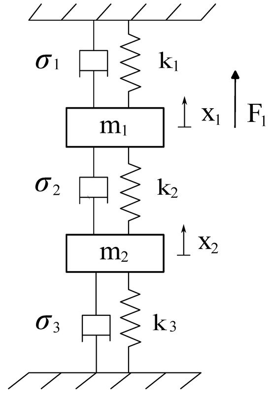
Figure 1.
A vibrating system with two degrees of freedom and viscous damping and a harmonic external force applied to the first mass.
Assume that the following simplified hypotheses are valid. The two particles have masses and and move along smooth guides, which are not shown in Figure 1. The springs depicted in Figure 1 can be approximated as massless elastic elements with stiffness values , , and , respectively, [82]. Based on these assumptions, the vibrating mechanism is simplified to a two-degrees-of-freedom system.
The two masses shown in Figure 1 are subjected to a linear elastic force field, a linear viscous force field, and harmonic excitation [83]. The elastic force field is represented by a spring with stiffness , located between mass and the ground; a spring with stiffness , situated between masses and ; and a spring with stiffness , positioned between mass and the ground [84]. The viscous force field is illustrated by a viscous damper with damping coefficient , placed between mass and the ground; a viscous damper with damping coefficient , situated between masses and ; and a viscous damper with damping coefficient , placed between mass and the ground. Furthermore, a harmonic excitation acting on the first mass is considered in the dynamic model, expressed as , where t is time, represents the magnitude of the external force, and denotes the angular frequency of the external excitation.
To define the specific configuration of the vibrating system at any given moment in time t, one can consider the displacements of the two masses, referred to as and , measured from their respective rest positions. Assuming the absolute displacements and to be the degrees of freedom of the system, one can write that
where is the generalized displacement vector of the vibrating system at hand.
The equations of motion for this vibrating mechanical system can be easily derived from the Euler–Lagrange equations. Generally, when working with a system characterized by n degrees of freedom, n nonlinear ordinary differential equations are necessary to describe the system dynamics accurately [85]. Consider the following general form of the vector of generalized coordinates for a dynamical system:
The Lagrange equations, which correspond to the minimal set of generalized coordinates introduced before, can be expressed as follows:
where T represents the system kinetic energy, V denotes the system Rayleigh dissipation function, U is the system potential energy, and is the system time-dependent generalized force vector describing the external excitation sources. In the case of the vibrating system under study, T corresponds to the total kinetic energy of the particles, U denotes the total potential energy of the springs, and V is the total power dissipated by the damping elements of the system. Therefore, by applying the Euler–Lagrange equations, one obtains
Furthermore, the equations of motion can be written in a matrix form as
where
and
where is the system mass matrix, is the system damping matrix, is the system stiffness matrix, and is the system force vector of external excitations. More specifically, the matrix equations given in Equation (5) correspond to the two scalar equations given in Equation (4).
2.2. Design of a Dynamic Vibration Absorber Without Damping
Consider now a single-degree-of-freedom undamped vibrating system, where the displacement is denoted by . This simplified system is characterized by a mass of suspended on an elastic element with stiffness . Assume a harmonic excitation acting on this vibrating system with an amplitude and a frequency . The equation of motion for this linear single-degree-of-freedom vibrating system is the following:
Once the transient has expired, this system displays a forced response with a frequency , which is identical to that of the forcing function, and a phase delay of with respect to the excitation force. The functional form of this forced response can be identified by an explicit time-dependent function as follows:
where X represents the amplitude of the forced response, which can be expressed in terms of the product of the dynamic amplification coefficient A and the so-called static deformation . For an undamped single-degree-of-freedom system, the dynamic amplification coefficient is given by
where represents the ratio between the excitation angular frequency and the natural angular frequency of the vibrating system given by . It can be inferred that, when the dimensionless ratio approaches a value of unity, the dynamic amplification coefficient of the system takes on high values, endangering the integrity of the system [86,87].
If an auxiliary vibrating system with a mass and an elastic stiffness is coupled to the primary vibrating system, the overall mechanical system becomes a two-degrees-of-freedom system, and its equations of motion are given by
The previous two scalar equations correspond to the following matrix equations expressed in a compact form:
where
and
Assuming the following harmonic solution:
It is possible to obtain the steady-state amplitudes of the forced vibrations of the two masses and as follows:
When introducing a dynamic vibration absorber, the main objective is to reduce the vibration amplitude of mass . To achieve this, adequately designing the parameters and of the auxiliary system connected to the primary system is paramount. To make the vibration amplitude of equal to zero, the numerator of the forced displacement given in Equation (16) should be set equal to zero [88]. This yields
Taking into account the worst-case scenario for designing a robust auxiliary system, it is assumed that the main structure operates at a frequency close to its resonance condition before the introduction of the dynamic vibration absorber [39]. Therefore, the absorber is designed such that
By doing so, the amplitude of vibrations of the main mass will be zero while operating at its original resonance frequency. Define now the natural frequencies of the primary mass and the auxiliary system taken on their own, as if they were two independent vibrating systems, as follows:
The two amplitudes of the forced displacements and given in Equation (16) can be written in the following form:
with
where and represent the dynamic amplification coefficients of the first and second mass, respectively, while represents the static deflection of the first mass. Representing the variation of the amplitude of vibrations of the main mass versus the dimensionless angular frequency ratio of the main mass , two peaks are obtained, which correspond to the natural frequency of the overall system.
As discussed previously, in principle, one obtains by setting . With this value of the angular frequency, the amplitude of the forced displacement of the second mass will be equal to the following:
which leads to
This result demonstrates that the force exerted by the auxiliary spring is in the opposite direction to the applied force, effectively canceling it out and causing to go to zero.
On the other hand, the following angular frequencies can be defined:
In this specific instance, the angular frequency represents the natural angular frequency of the dynamic vibration absorber, since . The two dynamic amplification coefficients defined earlier and denoted as and , owing to the inclusion of the auxiliary mechanical system, which is intended to function as a dynamic vibration absorber, can be alternatively expressed as follows:
where and are two coefficients having the dimensions of the fourth power of an angular frequency given by
The introduction of the dynamic vibration absorber transforms the peak of the modulus of the dynamic amplification coefficient A, associated with the primary system with one degree of freedom, into two peaks found in the moduli of the dynamic amplification coefficients and . These peaks characterize the forced response of the mechanical system with two degrees of freedom, created by combining the primary system with the auxiliary system [89,90]. However, these peaks are separated by a valley that, for , reaches zero in the case of the amplification coefficient , as the conditions of anti-resonance occur. This means that, if the physical parameters of the dynamic vibration absorber are designed in such a way that its natural angular frequency is equal to the angular frequency of the forcing function , the amplitude of vibration of the primary system becomes zero. In contrast, the dynamic vibration absorber connected to the primary system vibrates with a finite, non-zero amplitude equal to . From a physical perspective, the phenomenon that underlies the working principle of the dynamic vibration absorber is indeed feasible because the elastic response of the spring in the auxiliary system matches the external forcing function at each instant.
Operationally, the physical parameters of the absorber and are designed by first establishing the ratio between the auxiliary and primary masses, namely by setting (e.g., or ). Then, based on the knowledge of the angular frequency of the harmonic forcing function, one can obtain the numerical value of the parameter by setting , where represents the natural angular frequency of the auxiliary oscillator considered as a separate mechanical system. Therefore, it is possible to observe how the dynamic vibration absorber eliminates the given frequency but introduces two resonance frequencies and , at which the amplitude of the main mass vibrations becomes ideally infinite in the absence of damping.
In practice, the operating frequency must be kept away from the values of and . The values of and can be determined by setting the denominator of Equation (21) to zero. For this purpose, it is worth noting that
By setting the denominator of Equation (21) to zero.
The two roots of this equation are given by
It is important to observe that roots given in Equations (29) and (30) are functions of the dimensionless ratios and . When a damping source is introduced into the model of the dynamic vibration absorber, a modified version of Equations (29) and (30) will serve as the basis to design the optimal parameters of this auxiliary system.
2.3. Design and Optimization of a Dynamic Vibration Absorber with Damping
The dynamic vibration absorber described in the previous section can eliminate the original resonance peaks in the vibrational response of the primary mass. However, due to the lack of damping, this type of absorber simultaneously introduces two new peaks in the amplitude response of the primary system. Consequently, the primary system experiences high vibrational amplitudes as it traverses the two peaks during the start-up and shut-down phases. The amplitudes of the primary mass can be reduced by introducing a damper in conjunction with the auxiliary system, as illustrated in Figure 2.
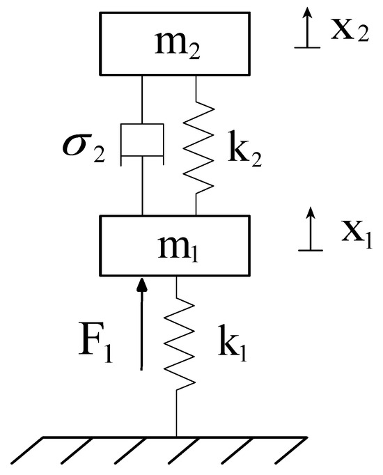
Figure 2.
Dynamic vibration absorber with viscous damping and a harmonic force applied to the first mass.
By adopting the same Lagrangian approach introduced above for the undamped absorber, the following expressions give the equations of motion for the two masses in the presence of damping and considering a harmonic external force :
Consider now a forced solution with the following analytical form:
where i is the imaginary unit. It is possible to obtain the steady-state solution of the two previously defined equations of motion given in Equation (31) as
and
In Equations (33) and (34), the focus is on the complex part of this solution. Define now the following dimensionless quantities:
and
Equation (35) shows how the dimensionless amplitude of the main mass is a function of the dimensionless parameters denoted with , , , and , which, respectively, represent the mass ratio, the angular frequency ratio, the forced frequency ratio, and the damping ratio.
Consider now a parametric study of the positive quantity in terms of the forced frequency ratio, for and for a few different values of . If the damping is zero, when , the resonance occurs at the two undamped resonance frequencies of the system. When damping becomes infinite, when , the two masses and are virtually locked together. In this second case, the system essentially behaves like a single-degree-of-freedom system with a combined mass and stiffness . Thus, resonance occurs with and g is equal to
Considering the effect of the dynamic vibration absorber with viscous damping on the response of the system through the parametric study of the positive quantity versus , the peak of is infinite for and . Somewhere between these limits, the peak of will be finite and small [91,92]. Furthermore, it can be observed that all curves pass through two points regardless of the damping value [91,92]. These points can be located by substituting the extreme cases of and into Equation (35) and equating them. This yields
The two roots of the equation indicate the values of the frequency ratio and corresponding to points A and B, which identify the points of the intersection found in the parametric study of the positive quantity in terms of the forced frequency ratio. The ordinates of A and B can be found by substituting the values of and into Equations (29) and (30), respectively. It has been observed that the most efficient vibration absorber is the one for which the ordinates of points A and B are equal [93]. This condition requires that
A dynamic vibration absorber that satisfies this equation can be called a tuned vibration absorber. Despite Equation (39) guiding tuning a mass damper, it does not specify the optimal damping ratio and the corresponding value of . The optimal value of can be found by ensuring that the curve representing the response is as flat as possible between the two points of intersection. This result can be achieved by making the curve horizontal at both the points of intersection A and B. To accomplish this, first, Equation (39) is substituted into Equation (35) to make the resulting equation applicable to the case of optimal tuning. Subsequently, the modified equation is differentiated with respect to g to find the slope of the curve of . Setting the slope equal to zero at the points A and B mentioned before, one obtains
and
where Equations (40) and (41), respectively, refer to points A and B. For engineering applications, a convenient average of two preceding values of is used in the design of a damped dynamic vibration absorber:
By doing so, the corresponding optimal value of becomes
As discussed in detail below, the virtual prototype of the case study and its corresponding mechanical model are respectively shown in Figure 3 and Figure 4, while the optimization condition for determining the dimensionless damping ratio is illustrated in Figure 5.
Figure 3.
Three-dimensional CAD model of the vibrating structure analyzed as the case study and the proposed system that serves as a dynamic vibration absorber.
Figure 4.
Lumped parameter model of the vibrating structure considered as the case study and the proposed system that serves as a dynamic vibration absorber.
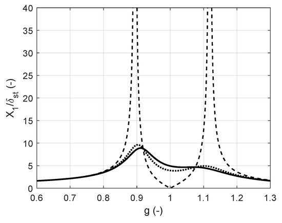
Figure 5.
Dynamic amplification coefficient of the primary mass in the absence of damping (dashed line), with non-optimized damping (dotted line), and with optimized damping (solid line).
3. Case Study
3.1. Description of the Case Study
This section aims to analyze the system selected as the case study for this paper objectively, focusing on the actual arrangement of its elements, depicted as masses and springs in the discretized system model. The goal is to validate the proposed auxiliary structure as a vibration absorber and demonstrate its applicability. In practice, this dynamic vibration absorber can be incorporated into the original design of the system. For this purpose, a three-dimensional CAD model of the vibrating structure, assumed to be the case study of the paper, along with the proposed design of a dynamic vibration absorber, is presented herein and is shown in Figure 3.
As shown in Figure 3, the mass–spring–damper system acting as a dynamic vibration absorber, connected to the primary system, is represented by a guyed mast structure consisting of a slender vertical rod with a circular cross-section and a spherical mass attached at its end. The connection of the slender vertical rod to the system is achieved using a joint through specific holes made at the locations of the spherical mass and the steel plate, as well as employing a threading process at the upper and lower ends of the cylindrical rod and the corresponding seat where the rod is positioned. This structure serves as an auxiliary system functioning as a dynamic vibration absorber. Consequently, it operates as a mechanical adjunct composed of inertia, stiffness, and damping elements that can absorb vibrational energy at the connection points once linked to the primary system. As a result, the primary system can be safeguarded from excessively high vibration levels.
Two parallel viscous dampers are integrated into the structure of the auxiliary system represented in Figure 3, functioning as dynamic vibration absorbers. Each viscous damper comprises a sealed piston that moves within a cylinder. One end of the cylinder is rigidly connected to the device, while the piston is attached to the other end. These viscous dampers dissipate a portion of the mechanical energy from the auxiliary vibrating system by converting it into heat, which helps to dampen the vibrations in the auxiliary system and enhances its performance. For selecting the cylinder–piston systems, a reference has been made to pistons typically found in kitchen cabinets, as they possess dimensions compatible with the characteristics of the case being considered. The connection of each of the two piston ends to the rectangular plate can be achieved using appropriate attachments, along with aluminum structures and commonly available screws. In contrast, the connection of each piston end to the spherical surface can be established by creating threaded holes within the sphere and threading the ends of the two cylinder–piston systems, enabling their connection to the spherical mass through screwing.
As discussed below, the simplified mechanical model of the case study, as shown in Figure 3, is identical to the scheme reported in Figure 2. The main components of the system include the primary mass, denoted by , the auxiliary mass–spring–damper system, and the elements that connect to the frame, which has an equivalent stiffness denoted by . The primary mass consists of an infinitely rigid steel plate forming the first floor of the vibrating structure. On the other hand, the mass–spring–damper system, connected to the primary system and serving as a dynamic vibration absorber, is represented by a guyed antenna structure. This auxiliary structure comprises a thin, circular-sectioned rod arranged vertically, with a stiffness , and a spherical mass attached to the free end of the rod.
While the flexibility of the antenna-like beam provides internal elasticity for the absorber, external damping is achieved through two viscous dampers. Each damper features a piston–cylinder system in which a viscous fluid governs the damping effect. The ends of both dampers connect to the spherical mass of the auxiliary system and the midpoint of the longer side of the rectangular plate, respectively, and they are inclined at the same angle to the horizontal plane. This configuration of the dampers in relation to the elements they connect to geometrically forms an isosceles triangle. As detailed below, these geometric factors will prove essential for accurately sizing the two dashpots.
A horizontal sinusoidal force applied to the main structure, denoted as , is also considered. Its intensity will be defined based on the empirical considerations specified in the following.
3.2. Structural System Dynamic Modeling
The representation of the frame structure assumed as the case study of the paper is shown in Figure 3 through CAD modeling. At the same time, a mechanical scheme of the same structural system is represented in Figure 4.
By examining Figure 3 and Figure 4, we can highlight how the continuous system, which serves as the case study, can be discretized to obtain the lumped-parameter model of the vibrating frame. For this purpose, consider the vibrating system depicted in Figure 4 and assume the validity of the following simplifying assumptions. The two masses and slide between smooth linear guides. The Bosch profiles forming the supporting structure of the system and the connecting element between the mass of the dynamic absorber and the plate can be modeled as fixed–fixed beams, and therefore treated as elastic connections without mass. Additionally, the plate is considered infinitely rigid, and the effect of gravity on the structure under examination is ignored due to the high axial stiffness of the structural beams. As shown in the representation of the CAD model of the structure in Figure 3, the base of the structure comprises four profiles that can be modeled as fixed beams. Since, by assumption, the plate is infinitely rigid, one can represent the basic structure consisting of the four profiles and the plate as four elastic springs whose stiffness is equivalent to the beams and one rigid body that can only vibrate horizontally.
The primary mass consists of an infinitely rigid steel plate with geometric dimensions of (length), (width), (thickness), and a mass . This mass is obtained by considering a steel density , and the calculation was carried out as follows:
and
The plate, in turn, is placed on a base consisting of four horizontal Bosch profiles in aluminum and four bars in harmonic steel arranged vertically. The four horizontal profiles and their corresponding vertical bars are connected through steel corner elements. In general, the Bosch profiles are characterized by exceptionally stable grooves and large flanges that allow for high loads in both static and dynamic loading conditions. Thus, the plate support is made using four Bosch profiles with dimensions of , groove , profile surface ), and second moment of area . In addition, the vertical bars in harmonic steel have a rectangular cross-sectional area of dimensions and a length .
Considering the primary structure as a combination of two shear-type frames with a known stiffness coefficient , the system can be mechanically modeled as two springs in parallel, each of which is, in turn, given by the parallel of the flexural (bending) stiffness of two vertical beams . Hence, the total system stiffness is equal to
being for the shear-type frame structure:
where for a clamped–clamped beam with an imposed unit displacement at one of its ends:
Using the previously defined numerical data, it is possible to calculate the second moment of area for the four vertical steel bars with a rectangular cross-section that represent the linear elastic elements in the lumped-parameter model:
Therefore, the total stiffness of the primary mass–spring system is equal to
The numerical information necessary to define the geometry of the auxiliary mass–spring–damper system was established based on considerations regarding the material selection for the circular-sectioned bar supporting the secondary mass and through an optimization process of the stiffness and damping parameters constituting the system. Specifically, for the construction of the circular-sectioned bar, polyethylene was used as the material, with a length , a diameter , and an elastic modulus . The choice of material type was made by conceptualizing the vertical bar as a cantilever beam and considering the relationship between the stiffness , the Young modulus , and the second moment of area through the well-known formula:
Assuming a circular cross-section with a known diameter of the cross-sectional area, one can calculate the second moment of area with the following formula:
Therefore, knowing the second moment of the area of the cross-section , one can readily compute the length from Equation (51):
The obtained length value is acceptable as it aligns with the overall dimensions of the entire structure. However, this viable result was achieved through an iterative process considering various materials. In this vein, materials with a high Young modulus, such as metals, are unsuitable for the construction of the bar, as they would lead to excessively high length values incompatible with the main structure dimensions. Furthermore, the chosen solution minimizes the spatial dimensions of the auxiliary system.
3.3. Design of the Auxiliary Dynamic Vibration Absorber
As discussed above, the auxiliary mass–spring–damper system, connected to the primary system, is represented by a guyed antenna-like structure consisting of a thin, vertical, circular-section rod and a spherical mass attached to its end. In this design solution, the damping is externally provided by two additional components and is of the viscous type. It is implemented through the two cylinder–piston systems, which can be conceptualized as a single damping system placed in parallel with the elastic component represented by the thin rod. In the absence of damping, the dynamic absorber functions only if the excitation frequency exactly matches the anti-resonance frequency of the vibrating system . The addition of damping allows an increase in the operating bandwidth of the primary system in a range centered around the point . However, this comes at the cost of not having a zero amplification coefficient in that interval, but one that is slightly different from zero.
A practical method to determine the damping value to be added to the auxiliary system forming the dynamic vibration absorber is to establish a specific damping factor , determine the critical damping of the considered auxiliary system on its own as , and calculate the damping value to be inserted into the system based on the formula . Therefore, the objective of this method is to ensure that the operating bandwidth of the dynamic vibration absorber is as wide as possible, paying the price of having a non-zero but small amplification coefficient, as mentioned earlier. This qualitatively corresponds to operating over a wide range of frequencies, where the response amplitude is non-zero but sufficiently small to effectively achieve dynamic absorption. By adopting this simple but effective approach, one can write
In civil engineering applications, the systems referred to are commonly termed underdamped systems, where the damping ratio is less than critical damping . It is observed that, for actual structures, the value of the damping ratio falls within the range .
Alternatively, a different approach to determining the optimal damping coefficient was analyzed in this paper using the following formula for optimal damping:
where . Employing the optimal value of the dimensionless damping given by Equations (42) and (55), one obtains
In Figure 5, the amplification coefficient of the primary system is depicted with and without the chosen optimal damping factor.
On the y axis of Figure 5, there is the module of the dynamic amplification factor related to the primary mass expressing a measure of the displacement of the main mass itself, while on the x axis, the forcing frequency ratio is represented, where is the natural angular frequency of the primary system considered independently.
Following the theory allowing for the definition of the optimal damping of the dynamic vibration absorber, considering the case where , that is, the case where the natural frequency of the dynamic absorber taken as a separate system is equal to the natural frequency of the primary structure, an optimal damping factor was selected for the design of the auxiliary system. This is consistent with the empirical criterion previously described for determining the damping coefficient. Based on this reasoning, the damping value was obtained through a simplified representation of the actual model, considering a lumped parameter model, and therefore, without taking into account the actual arrangement of dampers in the continuous system [94,95].
As mentioned in the preceding paragraphs, the two dampers are inclined at a certain angle relative to the horizontal plane so that the arrangement of the dampers relative to the elements connected to them allows the geometric reproduction of the configuration of an isosceles triangle. Therefore, based on the available numerical data, one can readily identify the values of the angles and that allow for calculating the actual values of the two damping coefficients starting from the optimized equivalent damping found before. It follows that
and
Denoting with the damping coefficient of the inclined damper, the equivalent damping coefficient equal to the optimal damping coefficient, and the inclination angle of the inclined damper, one can obtain the damping matrix considering the inclined dampers as follows:
The damping matrix arising from the use of inclined dampers, which is explicitly given in Equation (59), can be readily computed as shown below:
being
where is the damping matrix in the local coordinate system aligned with the axis of the dashpot, and is a proper rotation matrix that takes into account the inclination angle of the damper axis evaluated counterclockwise with respect to the direction of the solicitation associated with the system motion.
Through geometric considerations, the position vector of the application point on the primary system and, similarly, the position vector of the dynamic vibration absorber can be written as follows:
where and are proper geometric lengths associated with the abscissa of the points P and D. To find the displacement vector of the application points of the inclined damper, one can calculate
which leads to
Subsequently, the dissipated power V of each inclined damper can be expressed as
Finally, the dissipative term of the inclined damper in the equations of motion is given by
where it is assumed that . Considering the symmetry assumption with two identical branches for the inclined dashpots, one can proceed with the calculation of the damping coefficient as follows:
As previously highlighted, operationally, the physical parameters of the dynamic absorber, and , are designed by establishing the ratio between the auxiliary and primary masses, that is, by setting , and based on the knowledge of the angular frequency of the harmonic excitation, by setting , where represents the natural frequency of the auxiliary oscillator considered as a separate mechanical system. In light of this, it is possible to assign numerical values to the physical parameters through the following relationships:
where corresponds to the value of the angular frequency of the horizontal harmonic external excitation acting on the primary system represented by the mass . Therefore, one can write
By using the available numerical data, one has
It follows that
The evaluation of and are reported in Equation (71). Once the mass is defined as , it is possible to determine the volume and the radius of the spherical body constituting the mass based on the following relationships:
and
Regarding commercially available dampers compatible with the current system, cylinder–piston configurations similar to those used in kitchen cabinets or the trunk of cars were considered due to their available sizes matching the characteristics of the case study. Additionally, the connection of the pistons to the rectangular plate can be achieved using suitable aluminum structures and commonly accessible screws. Moreover, connecting the piston ends to the spherical surface can be accomplished by creating threaded holes within the sphere and screwing the ends of both cylinder–piston systems onto the spherical mass.
To recap, the numerical values of all the geometric and physical parameters defined herein for the lumped parameter model of the case study are reported in Table 1.

Table 1.
Numerical values of the physical parameters of the primary flexible system with the dynamic vibration absorber.
It is worth noting that the numerical values of the system parameters reported in Table 1 fully characterize, from a mechanical perspective, the dynamic model corresponding to the physical system associated with the virtual prototype CAD model shown in Figure 3. Specifically, the actual values of the physical parameters presented in Table 1 are derived from the detailed analysis of the case study and the structural calculations of this investigation provided in Section 3.
4. Numerical Results and Discussion
4.1. Description of the Numerical Experiments
This section addresses the vibrational analysis of the vibrating frame developed in this paper, with a particular focus on numerical results and discussions. First, the system is modeled using a lumped parameter approach, from which the equations of motion are derived to create a mathematical model. Next, the dynamic response, represented by the displacements of the two masses that comprise the system, is simulated using MATLAB and a SIMULINK model (https://it.mathworks.com/products/simulink.html, accessed on 18 May 2025). As discussed in detail in this section, several numerical simulations were performed to analyze the case study of this investigation in different scenarios of engineering interest.
The first part of this section briefly describes the case study with a base displacement imposed on the ground, thereby representing how a structure behaves under a seismic excitation. In the first scenario, the damping effect of the dynamic vibration absorber, represented by the piston–cylinder systems between the two masses that comprise the system, is neglected. The second scenario examines the same system, in which the damping effect of the piston–cylinder system between the two masses is incorporated, to demonstrate the improvement in dynamic absorber performance through numerical experiments. In the third scenario, a more realistic setting is considered, where the stiffness coefficient of the primary system is assumed to be unknown and is estimated through an applied system identification approach, leading to an optimal design of the dynamic vibration absorber based on an identified mechanical model of the structural system that serves as the case study of the paper. Finally, the last subsection presents a general discussion of the numerical results obtained.
4.2. First Scenario: Dynamic Vibration Absorber Design Without Damping
Consider a scenario in which the vibrating frame structure is equipped with a dynamic vibration absorber, as illustrated in Figure 6. This design, defined in the previous sections, comprises an additional auxiliary mass that can dampen the vibrations of the primary system represented by the rectangular plate with mass . The physical parameters utilized in the simulation are provided for completeness in Table 1.
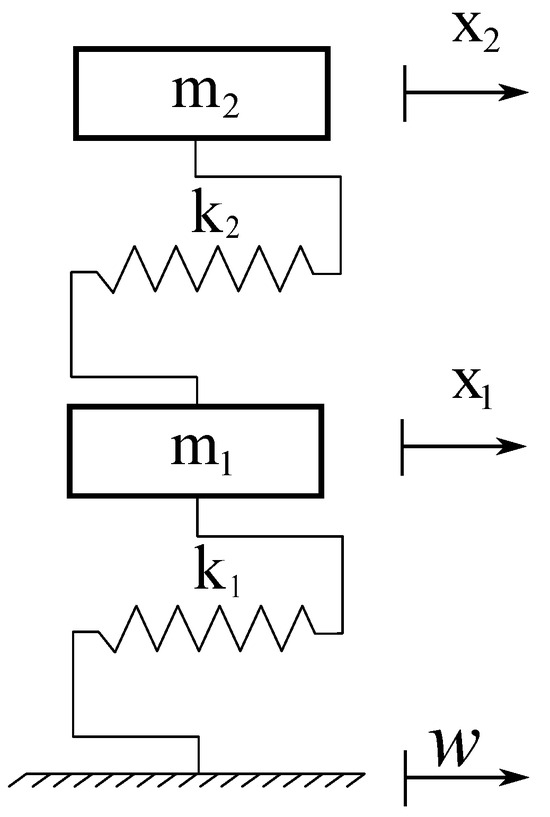
Figure 6.
Vibrating frame in the presence of the dynamic vibration absorber with a displacement imposed at the base and without damping.
In the model scheme illustrated in Figure 6, the system degrees of freedom include the horizontal displacements of the first and second masses, represented by and , respectively, where t identifies the time-independent variable, and w denotes the horizontal displacement of the ground. The configuration vector of the system is denoted as reported in Equation (1), where identifies the number of degrees of freedom of the structural system, indicates a time-dependent vector of dimensions representing the system generalized coordinate vector, while and , respectively, denote the time-dependent displacements of the first and second point masses, as mentioned before.
The dynamic model developed here can therefore be approximated as a simple system of two degrees of freedom with lumped parameters, and its mathematical modeling can be performed using the following equation of motion obtained through Lagrange equations:
where w is a known time-dependent function that plays the role of a forcing function. The two equations of motion allow for the mathematical modeling of the physical model of interest. In Equation (74), the presence of the time-dependent term w indicates the imposition of a displacement at the base described by a sinusoidal function defined as
being
where is the amplitude of the imposed displacement signal, L is the reference length of the vertical steel bars that form the frame structure assumed as the case study of the paper, is the angular frequency of the imposed motion, and is the natural frequency of the primary system considered individually. Once the form of the imposed displacement is defined, it is possible to substitute it into the equations of motion:
where . Considering the available data, the numerical values of the system mechanical parameters are reported in Table 2.
Table 2.
Vibrating system actual mechanical parameters without damping.
For simplicity, the possible presence of dissipative effects due to air resistance and friction forces was considered negligible, and the impact of viscous damping acting on the entire system was initially neglected in this first scenario.
To simulate the dynamic response of the system described mathematically, considering the dynamic model provided in Equation (74), it is possible to use a SIMULINK block program obtained by writing the two linear accelerations deduced from the equations of motion in the following explicit form:
Considering a simulation time of 30 (s) and an external excitation amplitude of , the graphical representations of the displacements, velocities, and accelerations of the system are shown in Figure 7, Figure 8 and Figure 9.
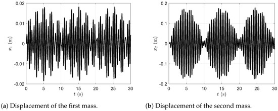
Figure 7.
Displacement of the first and second masses in the presence of the dynamic vibration absorber without viscous damping.
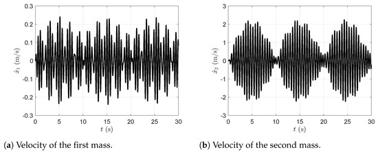
Figure 8.
Velocity of the first and second masses in the presence of the dynamic vibration absorber without viscous damping.
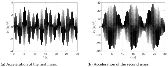
Figure 9.
Acceleration of the first and second masses in the presence of the dynamic vibration absorber without viscous damping.
Figure 7a represents the plot of the time evolution of the first mass displacement and Figure 7b represents the plot of the time evolution of the second mass displacement in the presence of the dynamic vibration absorber without viscous damping. Figure 8a represents the plot of the time evolution of the first mass velocity and Figure 8b represents the plot of the time evolution of the second mass velocity in the presence of the dynamic vibration absorber without viscous damping. Figure 9a represents the plot of the time evolution of the first mass acceleration and Figure 9b represents the plot of the time evolution of the second mass acceleration in the presence of the dynamic vibration absorber without viscous damping. All simulations were carried out with the dynamic vibration absorber and without considering viscous damping.
A state space representation of the equations of motion is considered to conveniently perform the modal analysis of the dynamic system under study. To this end, let be the dimension of the state-space and be a vector of dimensions representing the system state vector defined as
Defining as the number of degrees of freedom of the system and , the equations of motion that mathematically describe the mechanical model of the system at hand were previously defined in Equation (74). Thus, the matrix representation of Equation (74) can be readily expressed in the following form:
being
and
where is the externally applied force vector with dimensions , corresponding to the displacement imposed at the base, is the input collocation matrix with dimensions , where represents the number of inputs, F denotes the non-zero time-dependent input force, indicates the vector of generalized accelerations of the system, is the generalized velocity vector, represents the displacement vector of the two masses, denotes the mass matrix of the system, while represents the system stiffness matrix.
In this mathematical formulation, it is possible to determine the values of the physical terms within the matrices that define the system equations of motion, as reported in Table 2. Using classical methods of analytical dynamics, the mass and stiffness matrices can be defined as follows:
Given the definition of the system state vector and the structural matrices of the benchmark mechanical system, the principal continuous-time state-space matrices for its continuous-time representation can be derived as follows:
being
where is a square matrix of dimensions describing the system state matrix, is the input influence matrix of dimensions , is the input vector of dimensions , while and are proper zero and identity matrices having dimensions of , respectively.
In this study, the eigenvalues and eigenvectors of the matrix are computed using the MATLAB function eig. By doing so, the eigenvalues have the following complex conjugate pairs form:
where i is the imaginary unit, and it is understood that and are, respectively, the real and imaginary parts of the eigenvalue .
Knowing the general analytical form of the mechanical system eigenvalues, one can determine the natural angular frequency , the damping factor , and the natural frequency of each vibration mode j of the system, and the numerical results found are given in Table 3.
Table 3.
Physical parameters of the first and second normal modes without damping relative to the case study considered in the numerical analysis.
Since the eigenvalues occur in complex conjugate pairs, , , and also occur in pairs. Furthermore, from the theory of mechanical vibrations, it is well known that the eigenvector matrix relative to the system state-space mathematical coordinates has the following form:
where is a constant matrix of dimensions , representing the eigenvector matrix associated with the generalized coordinates of the system, and is a diagonal matrix whose diagonal entries are the eigenvalues . The matrix is arranged so that each odd column is the complex conjugate of the subsequent even column, maintaining this pattern for systems with multiple degrees of freedom. From the state-space eigenvector matrix , the state-space eigenvalue matrix , and the state-space block submatrix , one can extract the configuration-space eigenvector matrix of engineering interest by only selecting the odd columns of the matrix , as given below:
The configuration-space eigenvector matrix has dimensions , while and represent the first and second columns of the matrix and, respectively, describe the first and second normal modes of the flexible structure. The amplitude and phase corresponding to the first and second vibration modes can be obtained from the columns of these configuration-space eigenvectors. This is achieved by expressing the terms of the matrix in exponential form as follows:
with
and
In Equations (90) and (91), the terms and , respectively, represent the amplitude and the phase of the component j of the normal mode k, which are generally described by complex quantities. However, it is important to note that, since there are no damping effects in the first scenario considered herein, the phase angles assume, respectively, the values 0 and . In synthesis, the numerical results found from the present analysis to describe the physical parameters of the normal modes of the vibrating systems are reported in Table 3.
To facilitate the understanding of the modes of vibration reported in Table 3, it is common practice to normalize the values of the amplitude of the modes of vibration and consider the phases of the first mode shape as reference.
4.3. Second Scenario: Dynamic Vibration Absorber Design with Damping
This subsection considers the scenario where the vibrating frame structure is equipped with a dynamic vibration absorber having a damper, which was technically designed as shown in the previous sections. Consequently, the dynamic vibration absorber acts as an additional auxiliary mass , capable of dampening the vibrations of the primary system represented by the rectangular plate with mass in virtue of the adequately tuned additional stiffness and damping parameters, denoted by and .
In the model under consideration, only two degrees of freedom are defined by the horizontal displacements of the first and second masses, denoted by and , respectively. In this second scenario, the configuration and state vectors and of the mechanical system are identical to those considered in the first scenario, as given in Equations (1) and (79), respectively. Thus, even in this second scenario, the mechanical model of the structural system under study can be approximated as a lumped parameter system with two degrees of freedom, following the scheme shown in Figure 10.
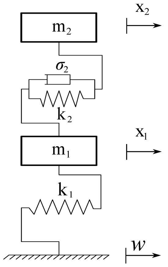
Figure 10.
Vibrating frame in the presence of the dynamic vibration absorber with a displacement imposed at the base and with damping.
The mathematical modeling of the vibrating system shown in Figure 10 can be carried out by considering the following equation of motion obtained from the use of Lagrange equations:
Considering the available data, the numerical values for the system’s mechanical parameters match those reported in Table 3, except for the value of the viscous damping coefficient of the auxiliary system, which is given as .
The system equations of motion given in Equation (92) can be readily rewritten in the following compact matrix form:
being
where , , and , respectively, denote the system mass, damping, and stiffness matrices of dimensions , while , and the forcing function due to the ground external motion is a vector of dimensions identical to the one given in Equation (81). Consequently, the system state matrix assumes the following block form:
Employing a procedure for the modal analysis that follows the same steps described in the previous subsection, one can easily find the system modal parameters in the presence of damping and considering the dynamic vibration absorber, as reported in Table 4.
Table 4.
Physical parameters of the first and second normal modes with damping relative to the case study considered in the numerical analysis.
On the other hand, to simulate the dynamic response of the system described mathematically by the two equations of motion given in Equation (92), it is possible to use a SIMULINK block program obtained by writing the system acceleration functions derived from the equations of motion in the following explicit form:
The two equations of motion allow for the definition of mathematical modeling of the system and to graphically represent, through a SIMULINK model that is numerically solved, the dynamic response describing the time responses of the two masses constituting the system. Considering a simulation time of 30 (s) again, the time evolutions shown in Figure 11, Figure 12 and Figure 13 are obtained, respectively, for the first and second masses.
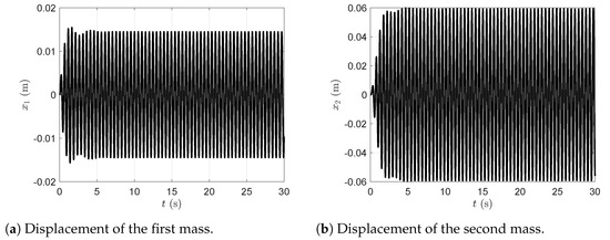
Figure 11.
Displacement of the first and second masses in the presence of the dynamic vibration absorber with viscous damping.
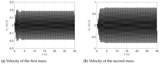
Figure 12.
Velocity of the first and second masses in the presence of the dynamic vibration absorber with viscous damping.
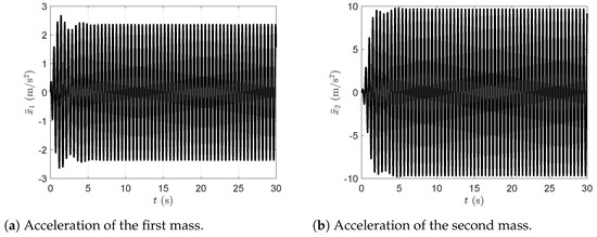
Figure 13.
Acceleration of the first and second masses in the presence of the dynamic vibration absorber with viscous damping.
Figure 11a represents the plot of the time evolution of the first mass displacement and Figure 11b represents the plot of the time evolution of the second mass displacement in the presence of the dynamic vibration absorber with viscous damping. Figure 12a represents the plot of the time evolution of the first mass velocity and Figure 12b represents the plot of the time evolution of the second mass velocity in the presence of the dynamic vibration absorber with viscous damping. Figure 13a represents the plot of the time evolution of the first mass acceleration and Figure 13b represents the plot of the time evolution of the second mass acceleration in the presence of the dynamic vibration absorber with viscous damping. All simulations were carried out with the dynamic vibration absorber and considering the viscous damping.
4.4. Third Scenario: Parametric Identification and Optimal Design
As discussed in this third and last scenario, the correct evaluation of system parameters is critical for the optimal design of the dynamic absorber. The mass of the system is generally easy to estimate, while the calculation of system stiffness is more complicated. Therefore, an identification procedure is proposed and analyzed in this section with the purpose of evaluating the stiffness of the primary system [96,97]. The approach adopted in this section is illustrated with the block diagram shown in Figure 14.
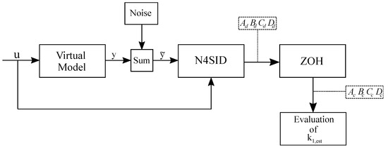
Figure 14.
Schematic diagram of the process employed for identifying the equivalent stiffness coefficient of the primary structure assumed as the case study of the paper.
The virtual model of the primary structure represents a one-degree-of-freedom vibrating system, as analyzed in Section 3. It consists of four pillars connecting a rigid base to the frame. The columns are modeled as flexible bodies, and the base is represented as a rigid body. To account for the energy dissipation, a proportional damping factor, expressed as , is introduced into the structural model so as to ensure a realistic representation of the dynamic behavior. In the simple proportional damping model considered herein for defining the system structural damping , the Rayleigh damping coefficients are denoted with and , where the former coefficient is associated with the primary system mass , while the latter coefficient is associated with the primary system stiffness . The physical parameters adopted for representing the virtual model are given in Table 5 for completeness.
Table 5.
Known and identified mechanical parameters of the vibrating system.
The virtual model receives in input an imposed motion given by the time law , which represents the force excitation signal and generates an output acceleration y corresponding to the input signal. The output acceleration is perturbed with a white noise having a mean parameter and the standard deviation parameter , which was appropriately chosen to simulate the uncertainties and disturbances typical of experimental measurements. Figure 15 shows the output acceleration signal disturbed by noise.
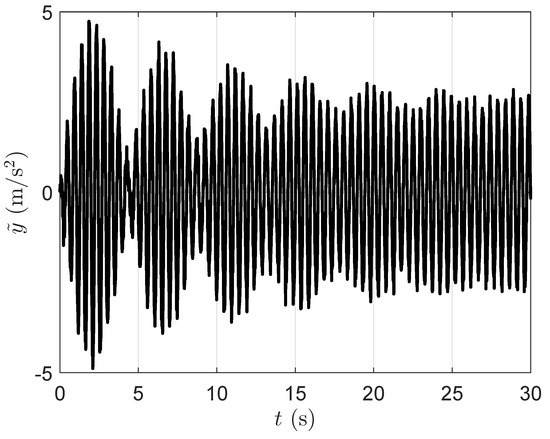
Figure 15.
Output acceleration of the virtual model disturbed by a white noise.
The accuracy of the measured signal can be readily evaluated by calculating the signal-to-noise ratio. This parameter indicates how predominant the relevant signal is over noise. The signal-to-noise ratio is expressed in decibels (dB) and is evaluated as follows:
where represents the mean of the squares of the output values, and denotes the mean of the squares of the noise values. A high index value indicates a clear signal with minimal interference. In the current case study, the observed value is 19.4866 (dB), confirming the consistency of the output evaluated by the virtual model. Therefore, it is possible to proceed to the next step in the workflow illustrated in Figure 14.
The first phase of the identification process involves employing an identification method to estimate the state-space model of the system. To achieve this, the investigation process adopted in this study utilizes a numerical procedure based on the N4SID (numerical algorithms for subspace state-space system identification) method [98]. The use of this algorithm facilitates the derivation of a model in the state space from the experimental input and output data [99]. Consequently, the output of the algorithm serves as a representation of the state space model of the system created from the experimental data. The discrete-time state-space representation of the identified dynamic model is as follows:
where k is the discrete-time index, is the discrete-time state vector, is the discrete-time input vector, is the discrete-time output vector, whereas , , , and represent the discrete-time state-space matrices obtained with the use of the N4SID method. For the sake of clarity, the subscript d indicates that the identified matrices belong to the discrete-time domain so as to not confuse them with their continuous-time counterparts marked with the subscript c.
The numerical results obtained for the identified matrices and are the following:
As previously mentioned, the model obtained using the N4SID method is in the discrete-time form. Therefore, it is necessary to convert it into a continuous model to analyze the dynamic properties of the system under study. This conversion is accomplished using the Zero-Order Hold (ZOH) reconstruction approach [100] and the discrete-continuous functional relationships implemented in the MATLAB function d2c, resulting in the continuous-time state-space formulation with the following analytical form:
where denotes the continuous-time state-space matrix, represents the continuous-time input influence matrix, connects the states to the measured outputs, and indicates the direct influence of inputs on the outputs. This form of the dynamical model provides a complete description of the system in the continuous state-space form. In particular, the numerical results obtained for the identified matrices and are presented in the following equation:
As discussed in Section 4.3, the eigenvalues and eigenvectors of the continuous-time state matrix are computed using the MATLAB function eig. Knowing the complex eigenvalue , one can easily calculate the natural angular frequency of the system as
where and represent the real and imaginary parts of the complex eigenvalue , respectively. Given the natural angular frequency of the system, it is easy to estimate the stiffness of the system as given in the following equation:
The evaluation of the relative error between the estimated stiffness and the actual stiffness of the virtual model is the following:
where denotes the estimated stiffness coefficient. This error in estimating the stiffness coefficient indicates the good accuracy of the identified state-space model, which deviates by % from the virtual stiffness coefficient .
Given the estimation of the system parameters, the criteria analyzed in this paper can be applied to evaluate the parameters of the dynamic absorber, as extensively discussed in Section 3.3. To facilitate the methodology explored in this study, the damping coefficient is neglected as it is quite small. It follows that
Figure 10 shows the lumped parameter model of the structural system obtained with these parameters. Hence, the mathematical modeling of the vibrating system can be carried out by considering the following equation of motion obtained from the use of Lagrange equations:
The dynamic response of the system is evaluated using a special-purpose program developed using SIMULINK (https://it.mathworks.com/products/simulink.html, accessed on 18 May 2025). Considering again a simulation time equal to 30 (s), the time evolution displacements shown in Figure 16, Figure 17 and Figure 18 are obtained, respectively, for the first and second masses.
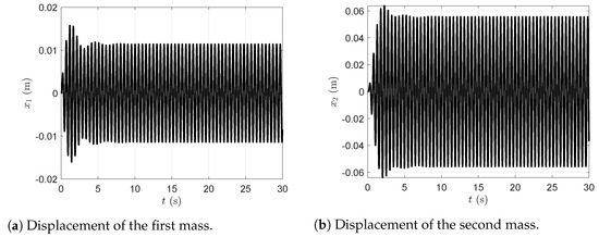
Figure 16.
Displacement of the first and second masses in the presence of the dynamic vibration absorber with viscous damping for the identification case.
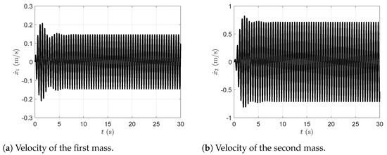
Figure 17.
Velocity of the first and second masses in the presence of the dynamic vibration absorber with viscous damping for the identification case.
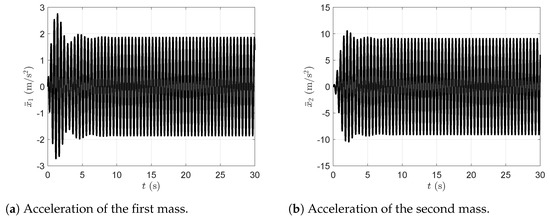
Figure 18.
Acceleration of the first and second masses in the presence of the dynamic vibration absorber with viscous damping for the identification case.
Figure 16a represents the plot of the time evolution of the first mass displacement and Figure 16b represents the plot of the time evolution of the second mass displacement in the presence of the dynamic vibration absorber with viscous damping for the identification case. Figure 17a represents the plot of the time evolution of the first mass velocity and Figure 17b represents the plot of the time evolution of the second mass velocity in the presence of the dynamic vibration absorber with viscous damping for the identification case. Figure 18a represents the plot of the time evolution of the first mass acceleration and Figure 18b represents the plot of the time evolution of the second mass acceleration in the presence of the dynamic vibration absorber with viscous damping for the identification case. All simulations were carried out with the dynamic vibration absorber and considering the viscous damping for the identification case.
4.5. Discussion and Final Remarks
The analysis of the first, second, and third scenarios demonstrates that the magnitudes of the oscillations of both masses decrease due to the damping effect of the piston-cylinder systems connected to the primary mass and the auxiliary system, respectively. More specifically, as shown in the two plots in Figure 11a,b, which illustrate the displacements of the masses comprising the primary mass and the auxiliary mass of the system, it is apparent how the transient related to the damping effects acting on the system diminishes almost instantaneously, allowing for the rapid attainment of the steady-state condition. Furthermore, by comparing the dynamic responses of the primary system and the auxiliary mass formed by the dynamic vibration absorber, it is observed that the auxiliary mass can independently dampen the vibrations of the primary mass, absorbing the vibrational forces acting on the system. This situation enables the supporting structure to operate safely, as it experiences lower vibrational forces than it would without a dynamic vibration absorber.
To quantify the effectiveness of the dynamic vibration absorber developed in this study, Table 6 presents the maximum amplitudes of the displacements, velocities, and accelerations of the first and second masses in all the scenarios analyzed in this investigation. In Table 6, Scenario 0 refers to the primary structure without the dynamic absorber; Scenario 1 refers to the primary structure with the dynamic absorber but without the auxiliary damping analyzed in Section 4.2; Scenario 2 refers to the primary structure with the dynamic absorber and the optimal damping analyzed in Section 4.3; and Scenario 3 refers to the identified dynamical model of the flexible system, comprising the primary structure and the optimally damped vibration absorber, analyzed in Section 4.4.
Table 6.
Maximum displacement, velocity, and acceleration values for the different cases analyzed in this investigation.
The numerical results reported in Table 6 were calculated using the following formulas:
where the subscripts j and k, respectively, identify the degree of freedom and the scenario analyzed, whereas , , and , respectively, denote the maximum displacement, velocity, and acceleration amplitudes in the four scenarios considered in this investigation.
Additionally, Table 7 compares the reductions in maximum displacement, velocity, and acceleration values across the various cases analyzed in this study.
Table 7.
Comparison of the maximum displacement, velocity, and acceleration reductions across the different cases analyzed in this investigation.
The performance parameters analyzed in this study, reported in Table 7 and used to compare scenarios 0, 1, 2, and 3, were assessed using the following equations:
In Table 7, represents the reduction in displacement amplitude of the first mass. Similarly, , also presented in Table 7, denotes the reduction in velocity amplitude of the first mass. Additionally, , referenced in Table 7, specifies the reduction in acceleration amplitude of the first mass. In Table 7, when one has , it indicates that the magnitude of the quantity in the Scenario k is smaller than the reference value.
5. Summary, Conclusions, and Future Work
In this investigation, a preliminary analysis focused on calculating the parameters that characterize the dynamic vibration absorber, to be integrated into a primary vibrating structural system, was carried out. At the same time, the functional validity of the dynamic vibration absorber was determined through a series of numerical simulations performed in the MATLAB environment (https://it.mathworks.com/products/matlab.html, accessed on 18 May 2025). These dynamic simulations enabled a comparison of the oscillations of the system masses with and without the dynamic absorber, emphasizing the advantages that could arise from its potential use. Specifically, the results of the numerical simulations facilitated both qualitative and quantitative comparisons between the dynamic responses of the primary system and the auxiliary mass represented by the dynamic absorber. This process allowed for observing how the auxiliary mass can dampen the vibrations of the primary mass independently, ensuring structural safety by reducing vibrational effects compared to scenarios without a dynamic absorber. Furthermore, the simulation results offered insights into how the dimensions of the structure, particularly the lengths of the harmonic steel vertical bars, relate to the magnitude of motion imposed at the base, thereby influencing the oscillations experienced by the system masses.
Another consideration involves the correlation between the materials used in the dynamic absorber and its dimensions. The choice of material arose from an iterative process that evaluated various options. It was noted that materials with a high Young’s modulus, such as metals, are unsuitable for constructing the vertical bar of the absorber because their excessively long lengths do not align with the dimensions of the structure outlined in the case study of this paper. Instead, plastic materials like high-density polyethylene were chosen for the circular section of the vertical bar to minimize spatial requirements. Furthermore, simplifications were made in the design of the dynamic vibration absorber, as well as in the subsequent computer-aided geometric modeling, omitting details regarding the anchoring and connection methods of the system components. This simplification aimed to create a viable virtual prototype design and validate its functionality through computer simulations. In effect, as a preliminary analysis, it can initially help to avoid precise definitions concerning the anchoring methods for the system components. For instance, the connection of the vertical thin rod to the system could be achieved by fitting it through specific holes made in the spherical mass and the steel plate while threading the upper and lower ends of the cylindrical rod into the seat where the rod is placed.
A crucial aspect examined in this investigation was the accurate estimation of the primary structure stiffness using a set of measured data for both input and output. This was accomplished through computer simulations that predicted the dynamic behavior of the central system in response to external excitation similar to seismic action while considering white noise as a source of disturbance. More specifically, a system identification procedure based on the N4SID method (numerical algorithms for subspace state-space system identification) implemented in MATLAB was employed to estimate the state-space model of the primary structural system. Subsequently, its structural parameters were extracted, allowing for the application of knowledge regarding structural topology and the calculation of the central frame mass through geometric and material considerations. Through this process, the estimated stiffness coefficient for the primary structure facilitated the design and testing of the dynamic vibration absorber under more realistic conditions. Even in this case, the numerical results obtained through computer simulations demonstrated the effectiveness of the dynamic vibration absorber in a more realistic scenario. Future research will focus on the experimental validation of the technical design solution developed in this study.
Author Contributions
This research paper was principally devised and developed by the first author (C.M.P.). Significant support in the development of the paper was provided by the second author (G.I.), the third author (A.D.), and the fourth author (R.L.R.). The detailed review carried out by the fifth author (V.P.B.) and by the sixth author (D.G.) considerably improved the quality of the work. The manuscript was written with substantial contributions from all authors. All authors reviewed the methodology, discussed the results, and approved the final version of the manuscript. All authors have read and agreed to the published version of the manuscript.
Funding
This research received no external funding.
Data Availability Statement
The data presented in this study are available from the corresponding author upon reasonable request.
Conflicts of Interest
The authors declare no conflicts of interest.
References
- Zuo, L. Effective and robust vibration control using series multiple tuned-mass dampers. J. Vib. Acoust. 2009, 131, 0310031. [Google Scholar] [CrossRef]
- Villecco, F. On the evaluation of errors in the virtual design of mechanical systems. Machines 2018, 6, 36. [Google Scholar] [CrossRef]
- Angeletti, F.; Iannelli, P.; Gasbarri, P.; Sabatini, M. End-to-end design of a robust attitude control and vibration suppression system for large space smart structures. Acta Astronaut. 2021, 187, 416–428. [Google Scholar] [CrossRef]
- Wei, L.; Zeng, J.; Huang, C.; Zheng, B.; Li, X. Hunting stability and dynamic stress analysis of a high-speed bogie using elastic-suspended motors as dynamic vibration absorber. Veh. Syst. Dyn. 2024, 62, 2332–2354. [Google Scholar] [CrossRef]
- De Piano, M.; Modano, M.; Benzoni, G.; Berardi, V.P.; Fraternali, F. A numerical approach to the mechanical modeling of masonry vaults under seismic loading. Ing. Sismica 2017, 34, 103–119. [Google Scholar]
- D’Ambrisi, A.; Mezzi, M.; Feo, L.; Berardi, V.P. Analysis of masonry structures strengthened with polymeric net reinforced cementitious matrix materials. Compos. Struct. 2014, 113, 264–271. [Google Scholar] [CrossRef]
- Berardi, V.P. Fracture failure modes in fiber-reinforced polymer systems used for strengthening existing structures. Appl. Sci. 2021, 11, 6344. [Google Scholar] [CrossRef]
- Qin, C.; Xu, A.; He, S.; Han, C.; Xu, Z. Virtual Dynamic Vibration Absorber Trap Fusion Active Vibration Suppression Algorithm Based on Inertial Actuators for Large Flexible Space Trusses. Aerospace 2024, 11, 764. [Google Scholar] [CrossRef]
- Li, F.; Wu, H.; Liu, L.; Ye, Y.; Wang, Y.; Wu, P. Nonlinear optimal frequency control for dynamic vibration absorber and its application. Mech. Syst. Signal Process. 2025, 223, 111932. [Google Scholar] [CrossRef]
- Park, M.H.; Yeo, S.; Choi, J.H.; Lee, W.J. Review of noise and vibration reduction technologies in marine machinery: Operational insights and engineering experience. Appl. Ocean. Res. 2024, 152, 104195. [Google Scholar] [CrossRef]
- Frahm, H. Device for Damping Vibrations of Bodies. US Patent 989,958, 18 April 1911. [Google Scholar]
- Rączka, W. Controlled SMA spring in Frahm’s vibration absorber. Mech./Akad. GóRniczo-Hut. Im. St. Staszica 2003, 22, 389–394. [Google Scholar]
- Bekdaş, G.; Nigdeli, S.M. Estimating optimum parameters of tuned mass dampers using harmony search. Eng. Struct. 2011, 33, 2716–2723. [Google Scholar] [CrossRef]
- Gutierrez Soto, M.; Adeli, H. Tuned mass dampers. Arch. Comput. Methods Eng. 2013, 20, 419–431. [Google Scholar] [CrossRef]
- De Simone, M.C.; Veneziano, S.; Guida, D. Design of a non-back-drivable screw jack mechanism for the hitch lifting arms of electric-powered tractors. Actuators 2022, 11, 358. [Google Scholar] [CrossRef]
- Tsai, H.C. The effect of tuned-mass dampers on the seismic response of base-isolated structures. Int. J. Solids Struct. 1995, 32, 1195–1210. [Google Scholar] [CrossRef]
- De Simone, M.C.; Veneziano, S.; Pace, R.; Guida, D. Multibody Analysis of Sloshing Effect in a Glass Cylinder Container for Visual Inspection Activities. Appl. Sci. 2024, 14, 4522. [Google Scholar] [CrossRef]
- Li, Y.; Zhang, Q.; Xu, Y.; Wen, J.; Wang, Z. Performance Evaluation of Inerter-Based Dynamic Vibration Absorbers for Wind-Induced Vibration Control of a Desulfurization Tower. Buildings 2024, 14, 150. [Google Scholar] [CrossRef]
- Cammarata, A.; Sinatra, R.; Rigano, A.; Lombardo, M.; Maddio, P.D. Design of a large deployable reflector opening system. Machines 2020, 8, 7. [Google Scholar] [CrossRef]
- Chen, X.; Kareem, A. Efficacy of tuned mass dampers for bridge flutter control. J. Struct. Eng. 2003, 129, 1291–1300. [Google Scholar] [CrossRef]
- Bertero, V.V. Performance-based seismic engineering: Conventional vs. innovative approaches. In Proceedings of the 12th World Conference on Earthquake Engineering, Auckland, New Zealand, 30 January–4 February 2000; Volume 30. [Google Scholar]
- Yao, J.T. Concept of structural control. J. Struct. Div. 1972, 98, 1567–1574. [Google Scholar] [CrossRef]
- Housner, G.; Bergman, L.A.; Caughey, T.K.; Chassiakos, A.G.; Claus, R.O.; Masri, S.F.; Skelton, R.E.; Soong, T.; Spencer, B.; Yao, J.T. Structural control: Past, present, and future. J. Eng. Mech. 1997, 123, 897–971. [Google Scholar] [CrossRef]
- Housner, G.; Soong, T.; Masri, S. Second generation of active structural control in civil engineering. Comput.-Aided Civ. Infrastruct. Eng. 1996, 11, 289–296. [Google Scholar] [CrossRef]
- Ikeda, Y.; Sasaki, K.; Sakamoto, M.; Kobori, T. Active Mass Driver System as the First Application of Active Structural Control; Wiley Online Library: Hoboken, NJ, USA, 2001; Volume 30, pp. 1575–1595. [Google Scholar]
- Anderson, T. Theme issue: Seismic isolation. Earthq. Spectra EERI 1990, 6, 438. [Google Scholar]
- Hanson, R. Theme issue: Passive energy dissipation. Earthq. Spectra 1993, 9, 319–636. [Google Scholar] [CrossRef]
- Soong, T.T.; Dargush, G.F. Passive Energy Dissipation Systems in Structural Engineering; Wiley: Hoboken, NJ, USA, 1997. [Google Scholar]
- Beltran-Carbajal, F.; Abundis-Fong, H.F.; Trujillo-Franco, L.G.; Yañez-Badillo, H.; Favela-Contreras, A.; Campos-Mercado, E. Online frequency estimation on a building-like structure using a nonlinear flexible dynamic vibration absorber. Mathematics 2022, 10, 708. [Google Scholar] [CrossRef]
- Constantinou, M.C.; Soong, T.T.; Dargush, G.F. Passive Energy Dissipation Systems for Structural Design and Retrofit; MCEER: Buffalo, NY, USA, 1998. [Google Scholar]
- Kassem, M.; Yang, Z.; Gu, Y.; Wang, W. Modeling and control design for flutter suppression using active dynamic vibration absorber. J. Vib. Eng. Technol. 2021, 9, 845–860. [Google Scholar] [CrossRef]
- Chang, C.; Yang, H.T. Control of buildings using active tuned mass dampers. J. Eng. Mech. 1995, 121, 355–366. [Google Scholar] [CrossRef]
- Yang, F.; Sedaghati, R.; Esmailzadeh, E. Vibration suppression of structures using tuned mass damper technology: A state-of-the-art review. J. Vib. Control. 2022, 28, 812–836. [Google Scholar] [CrossRef]
- Marano, G.C.; Greco, R.; Chiaia, B. A comparison between different optimization criteria for tuned mass dampers design. J. Sound Vib. 2010, 329, 4880–4890. [Google Scholar] [CrossRef]
- Rahimi, F.; Aghayari, R.; Samali, B. Application of tuned mass dampers for structural vibration control: A state-of-the-art review. Civ. Eng. J. 2020, 1622–1651. [Google Scholar] [CrossRef]
- Soong, T.T.; Spencer Reviewer, B., Jr. Active structural control: Theory and practice. J. Eng. Mech. 1992, 118, 1282–1285. [Google Scholar] [CrossRef]
- Chang, J.C.; Soong, T.T. Structural control using active tuned mass dampers. J. Eng. Mech. Div. 1980, 106, 1091–1098. [Google Scholar] [CrossRef]
- Nishimura, I.; Kobori, T.; Sakamoto, M.; Koshika, N.; Sasaki, K.; Ohrui, S. Active tuned mass damper. Smart Mater. Struct. 1992, 1, 306. [Google Scholar] [CrossRef]
- Preumont, A. Vibration Control of Active Structures; Springer: Berlin/Heidelberg, Germany, 1997; Volume 2. [Google Scholar]
- Yang, J.N.; Soong, T.T. Recent advances in active control of civil engineering structures. Probabilistic Eng. Mech. 1988, 3, 179–188. [Google Scholar] [CrossRef]
- Pourzeynali, S.; Lavasani, H.H.; Modarayi, A. Active control of high rise building structures using fuzzy logic and genetic algorithms. Eng. Struct. 2007, 29, 346–357. [Google Scholar] [CrossRef]
- Gransden, D.I.; Alderliesten, R. Development of a finite element model for comparing metal and composite fuselage section drop testing. Int. J. Crashworthiness 2017, 22, 401–414. [Google Scholar] [CrossRef]
- Leung, A.Y.T.; Zhang, H. Particle swarm optimization of tuned mass dampers. Eng. Struct. 2009, 31, 715–728. [Google Scholar] [CrossRef]
- Bakre, S.; Jangid, R. Optimum parameters of tuned mass damper for damped main system. Struct. Control. Health Monit. Off. J. Int. Assoc. Struct. Control. Monit. Eur. Assoc. Control. Struct. 2007, 14, 448–470. [Google Scholar] [CrossRef]
- Garrido, H.; Curadelli, O.; Ambrosini, D. Improvement of tuned mass damper by using rotational inertia through tuned viscous mass damper. Eng. Struct. 2013, 56, 2149–2153. [Google Scholar] [CrossRef]
- Aldemir, U. Optimal control of structures with semiactive-tuned mass dampers. J. Sound Vib. 2003, 266, 847–874. [Google Scholar] [CrossRef]
- Abé, M.; Fujino, Y. Dynamic characterization of multiple tuned mass dampers and some design formulas. Earthq. Eng. Struct. Dyn. 1994, 23, 813–835. [Google Scholar] [CrossRef]
- Igusa, T.; Xu, K. Vibration control using multiple tuned mass dampers. J. Sound Vib. 1994, 175, 491–503. [Google Scholar] [CrossRef]
- Luft, R.W. Optimal tuned mass dampers for buildings. J. Struct. Div. 1979, 105, 2766–2772. [Google Scholar] [CrossRef]
- Fujino, Y.; Abé, M. Design formulas for tuned mass dampers based on a perturbation technique. Earthq. Eng. Struct. Dyn. 1993, 22, 833–854. [Google Scholar] [CrossRef]
- Zuo, L.; Nayfeh, S.A. Optimization of the individual stiffness and damping parameters in multiple-tuned-mass-damper systems. J. Vib. Acoust. 2005, 127, 77–83. [Google Scholar] [CrossRef]
- Zou, D.; Haack, C.; Bishop, P.; Bezabeh, A. Damage criticality and inspection concerns of composite-metallic aircraft structures under blunt impact. In Proceedings of the Structural Health Monitoring and Inspection of Advanced Materials, Aerospace, and Civil Infrastructure 2015, SPIE, San Diego, CA, USA, 9–12 March 2015; Volume 9437, pp. 64–80. [Google Scholar]
- Shen, W.; Long, Z.; Cai, L.; Niyitangamahoro, A.; Zhu, H.; Li, Y.; Qiu, C. An inerter-based electromagnetic damper for civil structures: Modeling, testing, and seismic performance. Mech. Syst. Signal Process. 2022, 173, 109070. [Google Scholar] [CrossRef]
- Kang, B.H.; Hwang, J.H.; Choi, S.B. A new design model of an MR shock absorber for aircraft landing gear systems considering major and minor pressure losses: Experimental validation. Appl. Sci. 2021, 11, 7895. [Google Scholar] [CrossRef]
- Soong, T.; Reinhorn, A.; Aizawa, S.; Higashino, M. Recent structural applications of active control technology. J. Struct. Control. 1994, 1, 1–21. [Google Scholar] [CrossRef]
- Nishitani, A.; Inoue, Y. Overview of the application of active/semiactive control to building structures in Japan. Earthq. Eng. Struct. Dyn. 2001, 30, 1565–1574. [Google Scholar] [CrossRef]
- De Simone, M.C.; Rivera, Z.; Guida, D. A New Semi-Active Suspension System for Racing Vehicles. FME Trans. 2017, 45, 578–584. [Google Scholar]
- Ha, S.I.; Yoon, G.H. Numerical and experimental studies of pendulum dynamic vibration absorber for structural vibration. J. Vib. Acoust. 2021, 143, 011013. [Google Scholar] [CrossRef]
- Nagase, T.; Hisatoku, T. Tuned-pendulum mass damper installed in crystal tower. Struct. Des. Tall Build. 1992, 1, 35–56. [Google Scholar] [CrossRef]
- Gerges, R.R.; Vickery, B.J. Optimum design of pendulum-type tuned mass dampers. Struct. Des. Tall Spec. Build. 2005, 14, 353–368. [Google Scholar] [CrossRef]
- Matta, E.; De Stefano, A. Robust design of mass-uncertain rolling-pendulum TMDs for the seismic protection of buildings. Mech. Syst. Signal Process. 2009, 23, 127–147. [Google Scholar] [CrossRef]
- Almazán, J.L.; Juan, C.; Inaudi, J.A.; López-García, D.; Izquierdo, L.E. A bidirectional and homogeneous tuned mass damper: A new device for passive control of vibrations. Eng. Struct. 2007, 29, 1548–1560. [Google Scholar] [CrossRef]
- Kim, H.; Adeli, H. Hybrid control of irregular steel highrise building structures under seismic excitations. Int. J. Numer. Methods Eng. 2005, 63, 1757–1774. [Google Scholar] [CrossRef]
- Elias, S.; Matsagar, V. Wind response control of tall buildings with a tuned mass damper. J. Build. Eng. 2018, 15, 51–60. [Google Scholar] [CrossRef]
- Al-Saif, K.; Aldakkan, K.; Foda, M. Modified liquid column damper for vibration control of structures. Int. J. Mech. Sci. 2011, 53, 505–512. [Google Scholar] [CrossRef]
- Sakai, F. Tuned liquid column damper-new type device for suppression of building vibration. In Proceedings of the First International Conference on High-Rise Buildings, Nanjing, China, 25–27 March 1989; pp. 926–931. [Google Scholar]
- Ghaemmaghami, A.; Kianoush, R.; Yuan, X.X. Numerical modeling of dynamic behavior of annular tuned liquid dampers for applications in wind towers. Comput.-Aided Civ. Infrastruct. Eng. 2013, 28, 38–51. [Google Scholar] [CrossRef]
- Sarkar, A.; Gudmestad, O.T. Pendulum type liquid column damper (PLCD) for controlling vibrations of a structure–Theoretical and experimental study. Eng. Struct. 2013, 49, 221–233. [Google Scholar] [CrossRef]
- Longarini, N.; Zucca, M.; Silvestro, G. The constructions vibration control by tuned mass dumper. In Proceedings of the IABSE Symposium Report, International Association for Bridge and Structural Engineering, Geneva, Switzerland, 23–25 September 2015; Volume 105, pp. 1–8. [Google Scholar]
- Braun, S.; Ewins, D.; Rao, S.S.; Leissa, A. Encyclopedia of Vibration; SSP Group: London, UK, 2002; Volumes 1–3. [Google Scholar]
- Heimbs, S.; Hoffmann, M.; Waimer, M.; Schmeer, S.; Blaurock, J. Dynamic testing and modelling of composite fuselage frames and fasteners for aircraft crash simulations. Int. J. Crashworthiness 2013, 18, 406–422. [Google Scholar] [CrossRef]
- Hiken, A. The evolution of the composite fuselage: A manufacturing perspective. Aerosp. Eng. 2017, 10, 77–91. [Google Scholar] [CrossRef]
- Johns, D. Simulating Em Shielding for Aeronautical Applications. Available online: https://interferencetechnology.com/simulating-em-shielding-aeronautical-applications/ (accessed on 17 August 2017).
- Zou, T.; Mou, H.; Feng, Z. Research on effects of oblique struts on crashworthiness of composite fuselage sections. J. Aircr. 2012, 49, 2059–2063. [Google Scholar] [CrossRef]
- Kareem, A.; Kline, S. Performance of multiple mass dampers under random loading. J. Struct. Eng. 1995, 121, 348–361. [Google Scholar] [CrossRef]
- Sextro, W. Friction Damping of Elastic Structures. In Dynamical Contact Problems with Friction. Lecture Notes in Applied Mechanics; Springer: Berlin/Heidelberg, Germany, 2002; pp. 85–108. [Google Scholar]
- Wang, J.; Shieh, W. The influence of a variable friction coefficient on the dynamic behavior of a blade with a friction damper. J. Sound Vib. 1991, 149, 137–145. [Google Scholar] [CrossRef]
- Pappalardo, C.M.; Vece, A.; Galdi, D.; Guida, D. Developing a reciprocating mechanism for the emergency implementation of a mechanical pulmonary ventilator using an integrated CAD-MBD procedure. FME Trans. 2022, 50, 238–247. [Google Scholar] [CrossRef]
- Calabrese, A.; Quaglini, V.; Strano, S.; Terzo, M. Online estimation of the friction coefficient in sliding isolators. Struct. Control. Health Monit. 2020, 27, e2459. [Google Scholar] [CrossRef]
- Calabrese, A.; Losanno, D.; Barjani, A.; Spizzuoco, M.; Strano, S. Effects of the long-term aging of glass-fiber reinforced bearings (FRBs) on the seismic response of a base-isolated residential building. Eng. Struct. 2020, 221, 110735. [Google Scholar] [CrossRef]
- Calabrese, A.; Gandelli, E.; Quaglini, V.; Strano, S.; Terzo, M.; Tordela, C. Monitoring of hysteretic friction degradation of curved surface sliders through a nonlinear constrained estimator. Eng. Struct. 2021, 226, 111371. [Google Scholar] [CrossRef]
- Gandelli, E.; Lomiento, G.; Quaglini, V.; Strano, S.; Terzo, M.; Tordela, C. Estimation of the instantaneous friction coefficients of sliding isolators subjected to bi-directional orbits through a nonlinear state observer. Eng. Struct. 2021, 249, 113374. [Google Scholar] [CrossRef]
- Palli, G.; Strano, S.; Terzo, M. A novel adaptive-gain technique for high-order sliding-mode observers with application to electro-hydraulic systems. Mech. Syst. Signal Process. 2020, 144, 106875. [Google Scholar] [CrossRef]
- Pappalardo, C.M.; Lök, Ş.İ.; Malgaca, L.; Guida, D. Experimental modal analysis of a single-link flexible robotic manipulator with curved geometry using applied system identification methods. Mech. Syst. Signal Process. 2023, 200, 110629. [Google Scholar] [CrossRef]
- Cammarata, A.; Sinatra, R.; Rigato, R.; Maddio, P.D. Tie-system calibration for the experimental setup of large deployable reflectors. Machines 2019, 7, 23. [Google Scholar] [CrossRef]
- Pappalardo, C.M.; Califano, F.; Lok, S.I.; Guida, D. A Systematic Computational and Experimental Study of the Principal Data-Driven Identification Procedures. Part I: Analytical Methods and Computational Algorithms. J. Appl. Comput. Mech. 2023, 9, 529–549. [Google Scholar]
- Pappalardo, C.M.; Califano, F.; Lok, S.I.; Guida, D. A Systematic Computational and Experimental Study of the Principal Data-Driven Identification Procedures. Part II: Numerical Analysis and Experimental Testing. J. Appl. Comput. Mech. 2023, 9, 550–589. [Google Scholar]
- Pappalardo, C.M.; La Regina, R.; Guida, D. Multibody modeling and nonlinear control of a pantograph scissor lift mechanism. J. Appl. Comput. Mech. 2023, 9, 129–167. [Google Scholar]
- Pinkaew, T.; Lukkunaprasit, P.; Chatupote, P. Seismic effectiveness of tuned mass dampers for damage reduction of structures. Eng. Struct. 2003, 25, 39–46. [Google Scholar] [CrossRef]
- Bekdaş, G.; Nigdeli, S.M. Mass ratio factor for optimum tuned mass damper strategies. Int. J. Mech. Sci. 2013, 71, 68–84. [Google Scholar] [CrossRef]
- McNamara, R.J. Tuned mass dampers for buildings. J. Struct. Div. 1977, 103, 1785–1798. [Google Scholar] [CrossRef]
- Elias, S.; Matsagar, V. Research developments in vibration control of structures using passive tuned mass dampers. Annu. Rev. Control. 2017, 44, 129–156. [Google Scholar] [CrossRef]
- Lee, C.L.; Chen, Y.T.; Chung, L.L.; Wang, Y.P. Optimal design theories and applications of tuned mass dampers. Eng. Struct. 2006, 28, 43–53. [Google Scholar] [CrossRef]
- Wu, S.; Li, H. A data-driven design method of distributed dynamic vibration absorber for broadband vibration suppression of thin-walled structures. Thin-Walled Struct. 2023, 182, 110264. [Google Scholar] [CrossRef]
- Strano, S.; Terzo, M. A multi-purpose seismic test rig control via a sliding mode approach. Struct. Control. Health Monit. 2014, 21, 1193–1207. [Google Scholar] [CrossRef]
- Keesman, K.J. System Identification: An Introduction; Springer Science & Business Media: London, UK, 2011. [Google Scholar]
- Simpkins, A. System identification: Theory for the user, (ljung, l.; 1999) [on the shelf]. IEEE Robot. Autom. Mag. 2012, 19, 95–96. [Google Scholar] [CrossRef]
- Van Overschee, P.; De Moor, B. Subspace Identification for Linear Systems: Theory—Implementation—Applications; Springer Science & Business Media: Berlin/Heidelberg, Germany, 2012. [Google Scholar]
- Juang, J.N. Applied System Identification; Prentice-Hall, Inc.: Englewood Cliffs, NJ, USA, 1994. [Google Scholar]
- Bernal, D. The zero-order hold in time domain identification: An unnecessary operating premise. Struct. Control. Health Monit. 2011, 18, 510–518. [Google Scholar] [CrossRef]
Disclaimer/Publisher’s Note: The statements, opinions and data contained in all publications are solely those of the individual author(s) and contributor(s) and not of MDPI and/or the editor(s). MDPI and/or the editor(s) disclaim responsibility for any injury to people or property resulting from any ideas, methods, instructions or products referred to in the content. |
© 2025 by the authors. Licensee MDPI, Basel, Switzerland. This article is an open access article distributed under the terms and conditions of the Creative Commons Attribution (CC BY) license (https://creativecommons.org/licenses/by/4.0/).