From Binary to Multi-Class: Neural Networks for Structural Damage Classification in Bridge Monitoring Under Static and Dynamic Loading

Abstract

Structural Health Monitoring (SHM) plays a vital role in ensuring the health status of a wide range of structures, such as bridges, buildings, and large infrastructure in general. The advantages of this process can be further enhanced by incorporating more numerical and statistical approaches into traditional methods, such as finite element analysis and Machine Learning. In this study, a truss bridge structure is examined, and neural networks are trained with data derived from finite element analyses under static loads and dynamic excitations. The contributions of this work are based on comparing neural networks trained with static and dynamic analyses, as well as deriving important insights into the key parameters that impact their performance in SHM. Initially, a binary classification problem is addressed, where numerically trained classifiers are tasked with identifying whether the structure is in a healthy state or not. This category is further divided into two subcategories, depending on the extent of the damage present in the structure. Subsequently, a multi-class classification problem is defined, where three different damage classes of the same extent are considered, and the trained network is required to distinguish between them. Although the training of all neural networks was highly satisfactory, the prediction results varied, with success rates ranging from 55% to 90%. Finally, conclusions are drawn from the results of the study regarding the model error influence, the impact of the damage size, and the types of neural networks and training data used.

1. Introduction

In the modern world we live in, as it has evolved, we observe all around us a wide range of engineering structures, from simple to extremely complex and intricate, serving various purposes. When it comes to large-scale structures such as bridges, buildings, and infrastructure, a critical field of engineering closely tied to these is Structural Health Monitoring (SHM) [1,2]. For mechanical systems with rotating components, this field is referred to as Condition Monitoring (CM). Both SHM and CM utilize engineering analysis methodologies that enable the assessment of the health status of the aforementioned structures and mechanical systems. Essentially, these methodologies are divided into two major stages. In the first stage, the necessary data regarding the structure’s response over a given period of time must be acquired, and in the second stage, the data are analyzed to draw conclusions about the presence and severity of potential damage in the structure.

The most important part of the SHM process is the acquisition or generation of the required data, as the subsequent steps depend on them [3]. Data acquisition can be carried out in two ways. The first way is the traditional method, where data are obtained through experimental measurements conducted on the physical structure or on a test model. The second method involves the use of computational and numerical techniques, such as the finite element method (FEM). Finite element models can be optimized through a process called model updating [4], which uses experimental data from the actual structure to ensure that the model behaves as closely as possible to reality. This allows for a wide range of analyses to be conducted, simulating various loading conditions and uncertainties in a cost-effective and time-efficient manner. Once the necessary data have been collected, the second stage in the damage detection process involves the appropriate processing and analysis of these data to detect any patterns that deviate from the healthy state and any anomalies. Various techniques are used for this purpose, such as signal analysis, statistical analysis, and Machine Learning (ML) models [5,6]. Through the use of Artificial Neural Network (ANN) models, numerical classifiers are implemented, which are ideal for detecting damage and, therefore, for addressing the problem of SHM [7,8].

It must be noted, however, that when an ANN is trained by FE data, it might not generalize properly on the corresponding experiment. This fact needs to be considered whenever synthetic data are used to train classifiers. However, limited cases in the literature exist that refer to it [9,10]. Therefore, based on the above review, a main problem of the SHM field that needs further investigation is the study of the modeling error effect when FE data are used. This can be especially interesting in applications such as bridge monitoring [11,12,13,14,15], where the structures are large and expensive and destructive testing for training data acquisition is not permitted, except in very special cases prior to decommissioning [14].

Outline of This Paper

This paper begins with the presentation of the bridge-like structure and the description of the process followed. The simple model and the actual model are defined, both referring to finite element models used to generate the training and validation data for the neural networks, respectively. Next, the training of the neural networks is conducted, first addressing the binary classification problem, followed by the multi-class classification problem. Finally, the results of the neural network predictions are presented, and conclusions are drawn regarding critical parameters that play a decisive role in their final performance.

The contributions of the present work in the literature can be summarized as the focus on the use of both static and dynamic response data, with a combination of robustness testing to modeling errors for FE-trained classifiers.

2. Methodology

2.1. Geometry and Materials

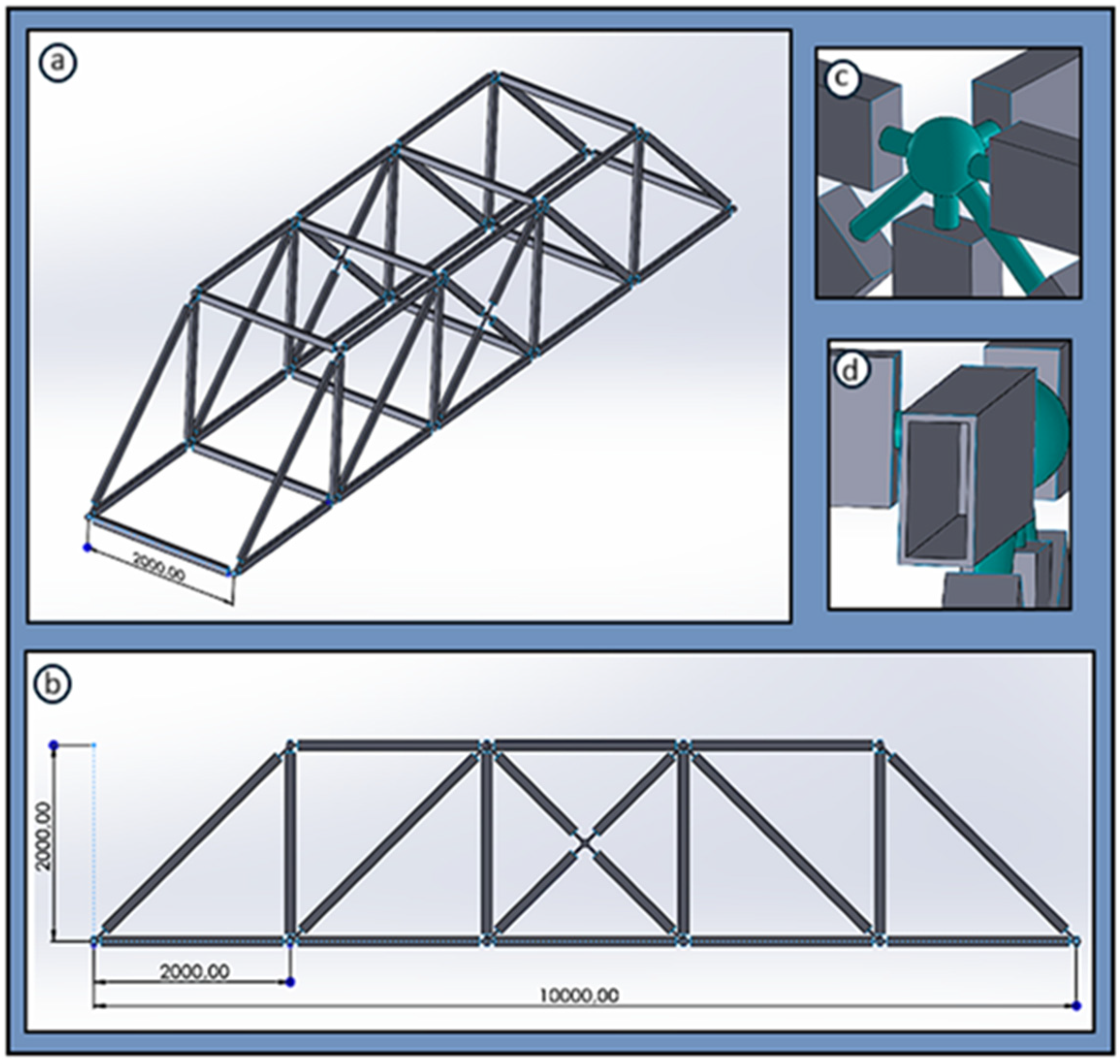
In the present work, the mechanical structure under examination is a footbridge, whose basic views, main dimensions, and certain design details are presented in Figure 1. This bridge is a space truss whose members have a hollow geometry and are connected at their ends using spherical joint connections. Its total length is 10 m, with a width and height of 2 m. The material chosen for the structure is a common steel with an elastic modulus of E = 210 GPa and a density of ρ = 7850 kg/m³.

Regarding the boundary conditions, the structure is supported by four edge nodes at its lower part, using fixed supports. The structural members of the bridge are primarily subjected to axial loads, but also to bending and torsional loads. Finally, uncertainties related to the structural characteristics of the structure are not considered in the present work.

2.2. Description of the Process

Initially, for the geometry of the bridge presented earlier, a suitable finite element (FE) algorithm is created in MATLAB, where the structure is simulated using one-dimensional rod elements (1D rod elements). Based on this modeling, the training data for the neural networks will be generated. Since we do not have an experimental setup available to evaluate the effectiveness of the trained neural networks, the experimental setup is substituted with simulations, which are conducted using commercial FE software, and more specifically ANSA v24 (BETA CAE Systems SA—Thessaloniki, Greece). Two-dimensional shell elements (2D shell elements) are chosen to model the experimental setup, rather than the one-dimensional elements used in the MATLAB model. This choice will affect the prediction accuracy results of the trained neural networks (model error influence). From this point forward, when referring to the “simple” model, the bridge model simulated in MATLAB with the one-dimensional rod elements is considered, whereas the “actual” model refers to the modeling implemented in the commercial software, which serves as the experimental setup.

In the Machine Learning part, two types of problems are addressed. The first is the binary classification problem, where two health states of the structure are defined (healthy or damaged), and the trained networks are tasked with determining the necessary “decision boundary” between them. Similarly, the multi-class classification problem is addressed, where three different damage classes of the same extent are defined, and the trained networks are required to identify and classify these distinct damage states. For both types of problems, neural networks are trained using data from static analyses, as well as Neural networks trained with data from dynamic analyses. In the case of the “statically” trained neural networks, their architecture follows the structure of deep neural networks (DNNs), utilizing fully connected layers. On the other hand, “dynamically” trained networks employ the structure of convolutional neural networks (CNNs), leveraging convolutional layers to extract information from the time-dependent data. This distinction allows the networks to process the different types of input data more effectively, enhancing their ability to classify the structural health conditions in both static and dynamic contexts. In all cases of the neural network architectures implemented, both in DNNs and CNNs, ReLU (Rectified Linear Unit) was used as the activation function for the neurons of the intermediate layers. Similarly, SoftMax was defined as the activation function for the output layers, given that the output in a classification problem must be a probability distribution. The number of training iterations, or epochs, was set as a hyperparameter for all networks. In the case of CNNs, the number of filters as well as their dimensions were also hyperparameters. Finally, the weight optimization algorithm chosen for the networks was Adam (Adaptive Moment Estimation).

3. “Simple” and “Actual” Models

3.1. “Simple” Model Implementation

The “simple” model refers to the simplified modeling using FE codes implemented in MATLAB, based on which the necessary static and dynamic analyses will be conducted and the training data for the neural networks will be derived. The bridge we are tasked with modeling forms a space truss. A truss is created by joining straight members at nodes, which are located at the ends of each member. The individual members of the space truss are two-force members, meaning that they are subjected to two equal and opposite forces directed along their axis. Therefore, each member is subjected only to axial loading. As a result, for this simplified modeling of the structure, 1Daxial rod elements were chosen for use.

The modeling of the structure begins with the appropriate numbering and naming of the members and nodes, respectively, as shown in Figure 2. This information must be arranged in a suitable format to be easily manageable by the FE codes that will be performed. Thus, two text files are created, containing information concerning the numbering and spatial arrangement of the nodes, as well as the connectivity between the members and nodes.

Regarding the boundary conditions, the bridge is supported at nodes A, F, L, and Q, where their degrees of freedom along the X, Y, and Z axes are constrained. Restricting rotation around the three axes is unnecessary, as the structure is a space truss modeled with axial rod elements, meaning that its members cannot resist bending and torsional moments. It is important to emphasize that the displacements of all nodes in the Y direction are restricted. This is necessary because, without these constraints, the model would be statically indeterminate.

3.1.1. Algorithm for Training Data Generation Using Static Analyses

The algorithm presented in Algorithm 1 below forms the basis for generating the training data from static analyses, which are used in the respective neural networks for their training and will be presented in the following sections. This algorithm defines a general code structure to be followed, where in each case the health state of the structure must be appropriately defined, as well as the labels that describe it.

Algorithm 1: Training Data Generation Using STATIC Analyses.

%Input: Number of analyses (n) and definition of the static loading matrix

%Output: Normalized results of ‘n’ analyses in a matrix form with the corresponding labels

1.   for i = 1 : n

2.   Define the properties $E$ (Young’s Modulus), $\rho$ (density), $A$ (cross section area)

3.   Define the geometry $g$.

4.   Define the health status with the corresponding labels

5.   Create the Stiffness matrix: $K=K(E,g)$

6.   Define the static loading vector: $\underset{˜}{F}$

7.   Apply the boundary conditions

8.   Solve the equation: $\underset{˜}{U}=K\backslash \underset{˜}{F}$

9.   Compute the stress of each element

10.  Normalize the results of displacements and stresses

11.  End

12.  Save the normalized results in a .csv file.

In each analysis, two nodes are randomly selected to which the static loads are applied. The random selection is made from all the nodes of the structure, excluding the fixed supports A, F, L, and Q. Furthermore, for a given analysis, it is not possible for the two randomly selected nodes to coincide. The forces applied have random magnitudes and directions (random components in the X and Z directions).

The normalization of the displacement results is achieved by dividing, in each individual analysis, the displacement values of all nodes (in the X and Z directions) by the maximum absolute displacement value observed at one of them. Similarly, the stresses of all members are normalized relative to the maximum absolute stress observed in one of them. This ensures that all stress and displacement values fall within a range of −1 to 1.

After the above algorithm is executed, the normalized results of the analyses are obtained in the form shown in Figure 3 and are saved in a .csv file.

3.1.2. Algorithm for Training Data Generation Using Dynamic Analyses

In Algorithm 2 below, the structure of the algorithm used to extract all the training data for neural networks trained with data from dynamic analyses is presented.

Algorithm 2: Training Data Generation Using DYNAMIC Analyses.

%Input: Number of analyses (n) and definition of the dynamic excitation matrix

%Output: Normalized displacement time series of the “sensors”, for ‘n’ analyses

1. for i = 1 : n

2.   Define the properties E (Young’s Modulus), ρ (density), A (cross section area), ζ (damping factor)

3.   Define the geometry g.

4.   Define the health status with the corresponding labels

5.   Create the Stiffness matrix: $K=K(E,g)$

6.   Create the Mass matrix: M

7.   Apply the boundary conditions

8.   Find the eigenfrequencies and eigenmodes by solving the eigenproblem: $(K-{\omega }^2{\rm M})\cdot \underset{˜}{\widehat{x}}=\underset{˜}{0}$

9.   Define the Damping matrix: C

10.  Define the simulation time and time steps

11.  Define the excitation vector: $\underset{˜}{f}(t)$

12.  Solve the set of equations: $M\cdot \underset{˜}{\ddot{x}}+C\cdot \underset{˜}{\dot{x}}+K\cdot \underset{˜}{x}=\underset{˜}{f}(t)$

13.  End

14.  Normalize the “sensors” response results and save them in .csv files.

In contrast to the static problem presented earlier (where loads were applied to randomly selected nodes in each analysis), in the case of the dynamic problem, two nodes are consistently selected to apply the excitations. Specifically, these nodes are Node C and Node O. Excitations are applied in both directions (X and Z) for both nodes. Figure 4a below schematically illustrates the excitations.

These excitations are defined as the sum of harmonic excitations and are given by the following expressions:

$$F_{cx}(t)=A_1\cdot \cos ({\omega }_1\cdot t)+\dots +A_{10}\cdot \cos ({\omega }_{10}\cdot t)$$

(1)

$$F_{cz}(t)=-(A_1\cdot \cos ({\omega }_1\cdot t)+\dots +A_{10}\cdot \cos ({\omega }_{10}\cdot t))$$

(2)

$$F_{ox}(t)=-(A_1\cdot \cos ({\omega }_1\cdot t)+\dots +A_{10}\cdot \cos ({\omega }_{10}\cdot t))$$

(3)

$$F_{oz}(t)=A_1\cdot \cos ({\omega }_1\cdot t)+\dots +A_{10}\cdot \cos ({\omega }_{10}\cdot t)$$

(4)

where $A_1$ to $A_{10}$ are random excitation amplitudes, and ${\omega }_1$ to ${\omega }_{10}$ the first ten natural frequencies of the structure derived from the FE software.

As “sensors”, the degrees of freedom of the nodes for which the displacement time histories will be recorded in each analysis are defined. Six nodes of the structure are selected: B, D, G, N, R, and U. This results in a total of 12 channels (two sensors for each node, corresponding to the X and Z directions), from which the response of the structure will be measured. For each channel, a matrix is created with n rows and t columns (3500 timesteps; 3.5 s total simulation time), where each row stores the response from a particular analysis. Once all analyses are completed, the response values in each matrix are normalized by the maximum absolute value recorded in each channel. This results in 12 normalized matrices containing the sensor responses from the n analyses. This separation of results into individual channels (Figure 5) is essential because the data are intended for training one-dimensional convolutional neural networks (1D CNNs), which require this format for input data.

3.2. “Actual” Model Implementation

After the necessary training of the neural networks, we are required to validate their effectiveness using data ideally derived from the actual structure or from an experimental setup. Since we do not have access to either of these setups, the structure is simulated using ANSA, utilizing 2D shell elements (Figure 6). This approach provides the model with greater realism compared to the “simple” model, as shell elements can handle not only axial loads but also transverse, bending, and torsional ones. Additionally, the bridge members have a hollow beam geometry with a relatively small thickness compared to the other two dimensions, making shell elements suitable for their description.

The modeling of the structure under examination is carried out using two-dimensional shell elements, specifically CQUAD4 elements. After the discretization of the geometry, the model consists of a total of 275,100 elements. Regarding their size, the shell element length is set to 10 mm.

To describe the connections between the structural members of the bridge (modeling of the spherical joint connections), Rigid Body Elements (RBE2) were used. These elements are connected to the members in the manner depicted in Figure 7a below. Subsequently, the appropriate boundary conditions are applied (Figure 7b). As explained earlier in the “simple” model, nodes A, F, L, and Q are fixed (all six degrees of freedom are constrained here), and the displacements of all nodes in the Y direction are restricted (to maintain consistency with the “simple” model).

Once the necessary procedure for creating the “actual” FE model of the structure is completed, the required static and dynamic analyses can be conducted. The results of these analyses will be used to evaluate the effectiveness of the trained neural networks. The outcomes from both the static and dynamic analyses are normalized and appropriately arranged with their respective labels to ensure full consistency with the corresponding data obtained from the analyses of the “simple” model.

4. Binary Classification Problem

The term “binary classification problem” refers to training a neural network to recognize patterns and trends in data, with the aim of categorizing the input into two classes (the structure is either healthy or damaged). In this section, neural networks will be trained using both static and dynamic data, enabling them to identify whether the bridge exhibits damage or remains in a healthy state.

This section is divided into two main subsections, with the key distinction being the severity of the damage in the structure. Section 4.1 focuses on neural networks trained with data where the structure is either healthy or has a “minor” damage, while in Section 4.2, the networks are trained similarly, but the damage is considered “extensive” in the damaged case.

4.1. Training of ANNs for Minor Damage Detection

As a “minor” damage scenario, we define a 90% reduction in the material’s modulus of elasticity for a randomly selected member. In each analysis of the bridge in a non-healthy state, one member is randomly chosen, and its modulus of elasticity is reduced by 90%.

In

Table 1. Information about the training of “minor” damage detection neural networks.

ANN Name	Type of FE Analysis	Neural Network Type	Number of Healthy State Analyses	Number of Damaged State Analyses	Training Dataset	Validation Dataset
Static_minor_damage_DNN	Static	Deep Neural Network (DNN)	2000	2000	3200 (80%)	800 (20%)
Dynamic_minor_damage_CNN	Dynamic	Convolutional Neural Network (CNN)	100	100	180 (90%)	20 (10%)

below, key information is provided regarding the training of two neural networks using data from static and dynamic analyses, respectively, for the detection of “minor” damage in the structure.

Below, in Figure 8, the architectures of the neural networks are presented. Additionally, in Figure 9, the training curves of these networks are displayed. The training curves provide valuable information regarding the learning performance of the networks.

4.2. Training of ANNs for Extensive Damage Detection

In the case of “extensive” damage, we assume that in the non-healthy state of the bridge, there are four beams with a reduced modulus of elasticity by 90%. Therefore, in each analysis concerning a damaged state of the bridge, four beams are randomly selected and are assigned a modulus of elasticity equal to 21 GPa.

Table 2. Information about the training of “extensive” damage detection neural networks.

ANN Name	Type of FE Analysis	Neural Network Type	Number of Healthy State Analyses	Number of Damaged State Analyses	Training Dataset	Validation Dataset
Static_extensive_damage_DNN	Static	Deep Neural Network (DNN)	2000	2000	3600 (90%)	400 (10%)
Dynamic_extensive_damage_CNN	Dynamic	Convolutional Neural Network (CNN)	100	100	160 (80%)	40 (20%)

provides information regarding the training of two neural networks, with data derived from static and dynamic analyses, concerning the diagnosis of significant damage in the structure.

Figure 10 and Figure 11 demonstrate the architecture and the training curves of the neural networks, respectively.

5. Multi-Class Classification Problem

The “multi-class classification problem” involves the training of two neural networks utilizing response data from static and dynamic analyses, respectively, which will be capable of recognizing and carrying out predictions for three different damage class scenarios in the bridge.

The three damage classes (Figure 12) that can occur in the bridge are defined as follows:

• Class 1: Members 11 and 43 (numbered according to Figure 2) have a 90% reduction in their modulus of elasticity.
• Class 2: Members 40 and 41 have a 90% reduction in their modulus of elasticity.
• Class 3: Members 17 and 18 have a 90% reduction in their modulus of elasticity.

Table 3. Information regarding the training of the multi-class neural networks.

ANN Name	Type of FE Analysis	Neural Network Type	Number of Class 1 Damage Analyses	Number of Class 2 Damage Analyses	Number of Class 3 Damage Analyses	Training Dataset	Validation Dataset
Multiclass_static_DNN	Static	Deep Neural Network (DNN)	2000	2000	2000	5400 (90%)	600 (10%)
Multiclass_dynamic_CNN	Dynamic	Convolutional Neural Network (CNN)	100	100	100	240 (80%)	60 (20%)

below provides the necessary information regarding the training of the two neural networks.

Figure 13 and Figure 14 below display the architecture of the networks and their training curves, respectively.

6. Results—Testing of the Trained Neural Networks

In this section, the effectiveness of the trained neural networks will be evaluated based on the corresponding data derived from static and dynamic analyses of the “actual” FE model of the structure. Subsequently, the results obtained are discussed.

6.1. “Binary Classification Problem”—Neural Network Testing

For the evaluation of each neural network model trained for the binary classification task, 10 analyses are conducted where the structure is in a healthy state and 10 where the structure is damaged (static or dynamic analyses, depending on the network for which they are intended). The results of these 20 analyses are fed into the neural networks, and the success of their predictions is assessed. Figure 15 presents the confusion matrices that demonstrate the prediction results.

Below, in

Table 4. Aggregate prediction results.

ANN Name	Damage Extent	Prediction Success Rate
Static_minor_damage_DNN	Minor	55%
Dynamic_minor_damage_CNN	Minor	80%
Static_extensive_damage_DNN	Extensive	75%
Dynamic_extensive_damage_CNN	Extensive	90%

, the prediction results of the neural networks are compiled.

From the above results, it can be observed that when comparing the neural networks trained with data from static analyses (DNNs), the network tasked with recognizing larger damages achieves a better prediction rate compared to the one for smaller damages, i.e., 75% versus 55%. The same trend is evident among the networks trained with dynamic analysis data (CNNs), where the success rates are 90% for large damages and 80% for smaller damages.

Therefore, in all cases, regardless of the type of network or the data used for its training, it is easier for a network to recognize a larger damage compared to a smaller one. This is easily explained and understood, as each neural network attempts to adjust its weights appropriately to find the suitable correlations that will lead to the correct separation between the two classes (healthy or damaged). Consequently, if the differences in the input data between classes 1 and 2 are very small (e.g., in the case of minor damage), the network will struggle to find the appropriate “borderline” between them. In contrast, with larger damage, the data become more distinct and clearer (showing more pronounced differences between the data of the two classes), making it easier to identify the features that distinguish it from the healthy state.

6.2. “Multi-Class Classification Problem”—Neural Network Testing

Similarly to the binary classification problem, for each of the three damage classes, 10 analyses are conducted based on the “actual” FE model of the structure. Therefore, a total of 30 analyses are generated (either static or dynamic, depending on the network for which they are intended), upon which the performance of the neural networks’ predictions is evaluated.

Below, in Figure 16 and Figure 17, the confusion matrices and the histograms of the prediction results are presented, respectively.

The trained network, Multiclass_static_DNN, achieves an overall prediction accuracy of 66.7%. This percentage does not represent a good predictive performance, especially considering that during the validation phase, the network achieved an accuracy of 98.33%. This indicates a poor correlation between the training data and the test data (high model error), meaning that the network does not generalize well.

We also observe, from both the bar charts and the confusion matrix data, that the network tends to predict two of the three classes with greater accuracy. Specifically, 90% of the data from class 3 and 80% from class 2 were predicted correctly. On the other hand, only 30% of the data from class 1 were accurately predicted. This reveals a clear “preference” of the network for distinguishing and recognizing classes 2 and 3 to a greater extent.

Similarly, the overall prediction accuracy of the trained network Multiclass_dynamic_CNN reaches 70%. Compared to the previous network, this one achieves relatively better performance. We observe that class 2 is predicted with 100% accuracy, while class 3 is predicted with 70% and class 1 with 40%. Thus, in this case too, the neural network shows a tendency to confuse class 1.

7. Discussion

The training and the effectiveness of a neural network in recognizing or detecting damage in structures, or more generally in mechanical engineering applications, is a problem influenced by many factors that clearly affect the performance and accuracy of the final predictions. Based on the analyses from the previous sections, certain conclusions were drawn regarding critical parameters that play a decisive role in the final performance of a network, which are outlined below.

• Model Error Influence

In general, the prediction performance of the trained neural networks was not as desired. This is primarily due to the model error that exists between the “simple” and the “actual” models. (From Figure 18, the discrepancy in the responses of the models for a given dynamic load becomes apparent, thus revealing the extent of the model error that exists.) It was observed that, while the accuracy of the networks’ predictions during training (on the validation dataset, consisting of data the network had not “seen” before, but coming from the same set as the training data) was above 96%, when they were fed with data from the real model’s analyses, the prediction rates were significantly lower. This indicates that the correlation between the training and test data is not satisfactory, despite the normalization of the data, which was an attempt to reduce, to some extent, the differences in the absolute values of the responses between the two models.

Thus, for the proper training and testing of neural networks, there needs to be as little model error as possible between the model used for generating training data and the real structure (this can be achieved by implementing model updating FE methods). This would maximize prediction performance and ensure greater reliability in the evaluation process. Additionally, it should be emphasized that potential discrepancies may arise between the simulated and real-world scenarios, such as various environmental factors (temperature, humidity, etc.), as well as the presence of noise that may distort the signals received by the sensors, making the inspection process even more demanding.

• Extent of the Damage

Regarding the size of the damage in the structure, the results of the neural networks evaluated in Section 6 revealed a clear trend. Specifically, in all cases, regardless of the type of network or the data used for training, it is easier for a network to recognize a larger damage compared to a smaller one. This can be explained and understood as the neural network adjusts its weights to find the correct correlations that allow for the proper separation between the two classes (healthy or damaged). When the differences in the input data between classes 1 and 2 are very small (as in the case of minor damage), the network struggles to find the appropriate “boundary” between them. On the other hand, in the case of more significant damage, the data become more distinct and clearer, making it easier to separate the features that differentiate it from the healthy state.

• Type of the Neural Network and Training Data

Among the neural networks trained in all cases, the convolutional neural networks (CNNs) used for dynamic analyses achieved higher prediction performance compared to the corresponding deep neural networks (DNNs) used for static analyses. This could be attributed to two main factors: the type of data used for training and the structure of the neural network itself.

Regarding the type of data, it is evident that dynamic analysis responses contain more information compared to static responses. Dynamic analyses provide insights into the inherent characteristics of the structure, such as natural frequencies, mode shapes, and damping properties. In contrast, static analyses yield constant and absolute values for displacements, stresses, and strains, which offer less additional information. However, a drawback of dynamic analyses is the increased time required to perform them, compared to static analyses. This is one of the primary reasons why training neural networks with static analysis data is also considered in this work.

Concerning the structure of the neural network, CNNs appear to outperform standard DNNs. CNNs incorporate convolutional layers in their architecture, which are capable of “scanning” the information and extracting useful features before proceeding to the fully connected layers. This gives CNNs the advantage of filtering the data and retaining only the useful information that aids in categorizing the different classes.

The contributions of the present work are based on the comparison of neural networks trained with static and dynamic analyses, as well as on drawing useful conclusions regarding critical parameters that determine their performance in SHM. As a foundation for future research, particular emphasis could be placed on the impact of various environmental factors and the minimization of modeling error between the simulation and the actual structure, as well as on modeling potential uncertainties related to the material properties of the structure itself, in order to create an SHM tool that will function seamlessly under real-world conditions.