Abstract
Marine propeller design requirements have risen in quantity and quality in recent decades. Reduced propeller cavitation is targeted to ensure that comfort requirements and environmental regulations are met. This paper presents the development of a mesh refinement process for the numerical prediction of tip vortex cavitation (TVC) using the commercial CFD package STAR-CCM+. Given the strong dependence on the mesh resolution within the areas of interest, mesh refinement and the use of field functions for adaptive meshing were demonstrated. The developed numerical model was substantiated against relevant published test data. Subsequently, the validated mesh refinement process was extended to scaled-up models representing medium- and full-scale propellers. The results showed that this process can be applied to CFD simulations to capture the minimum pressure within a tip vortex core. This process is also applicable to different types of hydrodynamic propulsors at both model scale and full scale. Additionally, the cavitation inception scaling law was evaluated for all small-scale and full-scale models, and it was found that the scaling parameter obtained using the developed refinement process was somewhat close to that obtained using existing methods. It is expected that the mesh refinement process developed in this study can be used to investigate the effect of scaling on tip vortex cavitation inception.
1. Introduction
Cavitation occurs when the fluid pressure drops below the local vapor pressure and is often an inevitable phenomenon for hydro machinery. It can have detrimental impacts on power and performance and is, therefore, a major limiting factor in the design of marine propulsion systems. The low-pressure core of a strong propeller tip vortex can initiate tip vortex cavitation, which can lead to excessive noise and vibration and cause erosion to the propulsor and the surrounding structures. The noise signature associated with the inception of a tip vortex cavity is of particular importance, as it can pose a significant threat to ocean wildlife, particularly marine mammals that rely on sound for communication [1,2]. The development of accurate and reliable techniques for the numerical prediction of tip vortex cavitation has, therefore, become an area of growing interest in recent years, as has assessment of the application of commercial CFD codes to cavitating propeller flows. Thanks to its advantages, CFD has also been widely used for other marine research, for example, Refs. [3,4,5].
Several studies on tip vortex cavitation (TVC) have been reported in the open literature [6,7,8]. From the relevant literature, it can be seen that prediction of a tip vortex cavity depends strongly on the mesh resolution within the vortex region [9,10]. Mesh refinement approaches have thus far focused on fixed volumetric refinements behind the propeller tip, requiring a priori knowledge of the flow field, and a mesh refinement cell size of D/1000 has been employed to resolve part of the tip vortex cavity [10]. Given the computationally demanding requirements of the mesh and the current limitations of the cavitation models, it is noted that there are still difficulties in numerically predicting the full extent of a downstream tip vortex cavity when using commercial CFD codes [11]. In order to predict the conditions for the onset of cavitation for full-scale vessels, a reliable scaling law for cavitation inception is required to scale from model tests to full-scale propellers. Deriving a suitable scaling law for cavitation inception using CFD has also been an area of interest within cavitation research [6,7].
From the preceding experimental studies, it is evident that TVC persists and travels a considerable distance in the propeller wake. While numerous studies have explored numerical simulations of TVC, the majority of these simulations have yielded unsatisfactory results, diverging significantly from observed experimental phenomena. Specifically, TVC tends to dissipate rapidly in the simulations, contrary to experimental findings [12,13,14]. A primary factor contributing to this discrepancy is the insufficient resolution of the computational mesh. To accurately simulate the roll-up and prolonged slip of TVC in a propeller wake, it is crucial to enhance the mesh resolution in the tip vortex wake region. Asnaghi et al. [15] conducted a combined numerical and experimental investigation into the inception behavior of TVC, demonstrating that TVC inception is closely linked to the size of the initial nuclei. Their findings indicated that a finer mesh resolution produces a stronger tip vortex, resulting in earlier TVC inception. In subsequent studies, different mesh resolutions were compared to analyze the vortex trajectory, streamwise velocity, and cavitation number, and this revealed that at least 16 mesh points are required per vortex radius to accurately predict the tip vortex and enable the axial acceleration velocity at the vortex core to be fully captured [16]. In efforts to improve TVC simulations, some researchers employed cylindrical geometry to refine the tip vortex mesh [17,18]. Despite these advances, while TVC behavior can be simulated, the detailed roll-up tip vortex phenomenon remains inadequately represented. Gaggero et al. [12] considered the impacts of transition models on cavitation inception and development, and found that modified models enhanced numerical predictions. However, discrepancies between simulated and experimental results persist for TVC extension.
Balze [19] analyzed the distinctions in simulation among the following three turbulence models: Direct Numerical Simulation (DNS) [20], Large-Eddy Simulation (LES) [21], and Reynolds-Averaged Navier–Stokes (RANS) equations. The RANS approach, introduced by Reynolds in 1895, involves decomposing flow variables into mean and fluctuating components, followed by time or ensemble averaging. This method allows for the use of considerably coarser grids compared with LES, and it assumes a stationary mean solution for attached or moderately separated flows. These characteristics significantly reduce the computational effort relative to LES or DNS, making the RANS approach highly popular in engineering applications. Sipilä and Siikonen [22] utilized RANS equations to investigate cavitating tip vortex flows in the Potsdam Propeller Test Case (PPTC). Their findings indicated that cavitating tip vortex simulations exhibit low sensitivity to the mass transfer rate. Further research by Sipilä et al. [23] revealed that different turbulence models significantly affect the solutions for tip vortex cores under both wet and cavitating conditions. Additionally, substantial discrepancies in pressure predictions within the wake region were observed among various RANS models. Specifically, the Explicit Algebraic Reynolds Stress Model (EARSM) predicted slightly lower pressures at the vortex core compared with the two-equation RANS models. Viitanen and Siikonen [24] conducted a comparative study of various turbulence models used to predict cavitating flows around the Potsdam Propeller Test Case (PPTC). The evaluated models included the low Reynolds number k − ϵ model, the SST k − ω model, the SST model with an Explicit Algebraic Reynolds Stress Model, and a Delayed Detached-Eddy Simulation (DDES) approach based on the SST k − ω model. The differences between the tested turbulence models in predicting global propeller performance were not substantial, although the k − ϵ model showed the best agreement with the experimental data. However, the tip vortex was generally underpredicted by all models.
This study aimed to employ a mesh refinement technique for the numerical prediction of tip vortex cavitation using the commercial CFD package Star-CCM+. Given the strong dependence on the mesh resolution within the areas of interest, this study focused on mesh refinement, and the effect of using field functions for adaptive meshing was investigated. Validation of the developed process was then performed by comparing it with relevant existing experimental data. The validated process was extended to scaled-up model propellers and discussed. The cavitation inception scaling law was also examined for all the small-scale and full-scale models. The capability of the developed refinement process in capturing the minimum pressure within the tip vortex core and its suitability for different types of hydrodynamic propulsors, at both model scale and full scale, are presented.
2. Development of the Mesh Refinement Process
2.1. Reference Experimental Propeller Model
In this study, a 5-bladed model-scale propeller tested by the Potsdam Propeller Test Case (PPTC) [25] was employed to develop a numerical model. The model-scale propeller was tested in both cavitating and non-cavitating conditions in the SVA Potsdam Model Basin. The results were presented at the 2011 Symposium on Marine Propulsors (smp’11) as validation data to aid the development of numerical methods for calculating the performance of marine propulsors [25]. Here, case 2.3.2 from the cavitating experiments was chosen as a basic case for the development of the refinement process, since, in this case, tip vortex cavitation visibly occurred, as revealed in Figure 1 [25]. The flow test conditions are given in Table 1.
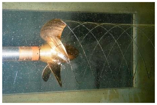
Figure 1.
A photo of downstream propeller wakes for case 2.3.2.

Table 1.
Test conditions for case 2.3.2.
2.2. Numerical Simulation
Numerical computations were performed using the flow solver STAR-CCM+ 13.04.011. The simulations were run for steady-state conditions with a single water phase. The rotation of the propeller was modeled using a rotating reference frame. The RANS (Reynolds-Averaged Navier–Stokes) K-Omega SST turbulence model was used with an all y+ wall treatment. A single-blade passage was modeled using periodic boundaries, as the blades were assumed to be identical. A polyhedral mesh was used for the propeller blade passage. The computational domain is shown in Figure 2, with the size defined according to the International Towing Tank Conference [26]. The single-blade passage boundaries are illustrated in Figure 3.
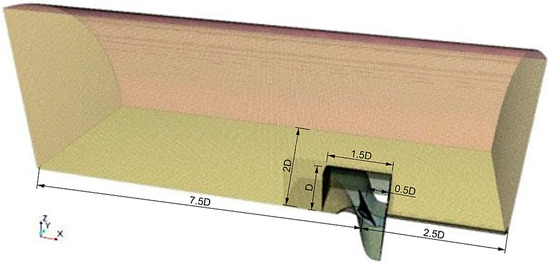
Figure 2.
Full computational domain. D denotes the propeller diameter.
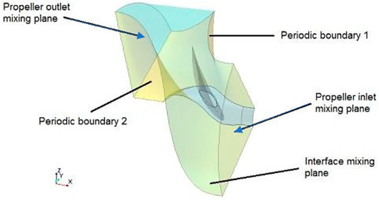
Figure 3.
Boundary conditions of a single-blade passage.
After the coarse mesh was created and the boundary conditions, numerical solution, and initial conditions were set up, the computational technique used to predict tip vortex patterns proceeded as follows:
Step 1: The solution was iterated until the convergence criteria were reached to obtain the solution for the coarse mesh (1000 iterations were used).
Step 2: The results of the initial simulation were analyzed to identify regions with significant flow features, such as regions with high velocity or pressure gradients (e.g., regions where tip vortex cavitation might occur).
Step 3: An adaptive mesh refinement technique [27] based on the local flow field was used. A table using field function criteria specified the cell size and the xyz coordinate position where the mesh region needed refinement. Subsequently, this table was used by the mesh generation tool in Star-CCM+. This tool used the table to adjust the mesh, making cells smaller in critical regions to capture more detail. After several iterations, the solution led to issues such as poor parallel processing efficiency and the creation of poor-quality cells due to large cell volume gradients.
An alternative technique also based on adaptive mesh refinement was explored to refine the mesh and capture the tip vortex core as follows:
Step 4: From an initial converged solution obtained on a coarse mesh in Step 1, volumetric threshold parts based on field functions of interest were determined. Next, the threshold parts were exported as STL files from the coarse converged solution.
Step 5: The STL files were imported into the initial solution from Step 1, and surface wrapping was used to ensure a closed volume.
Step 6: The simulation was run until convergence was achieved, and refinements were repeated iteratively, reducing the refinement cell sizes in each iteration until convergence of the minimum vortex pressure was achieved.
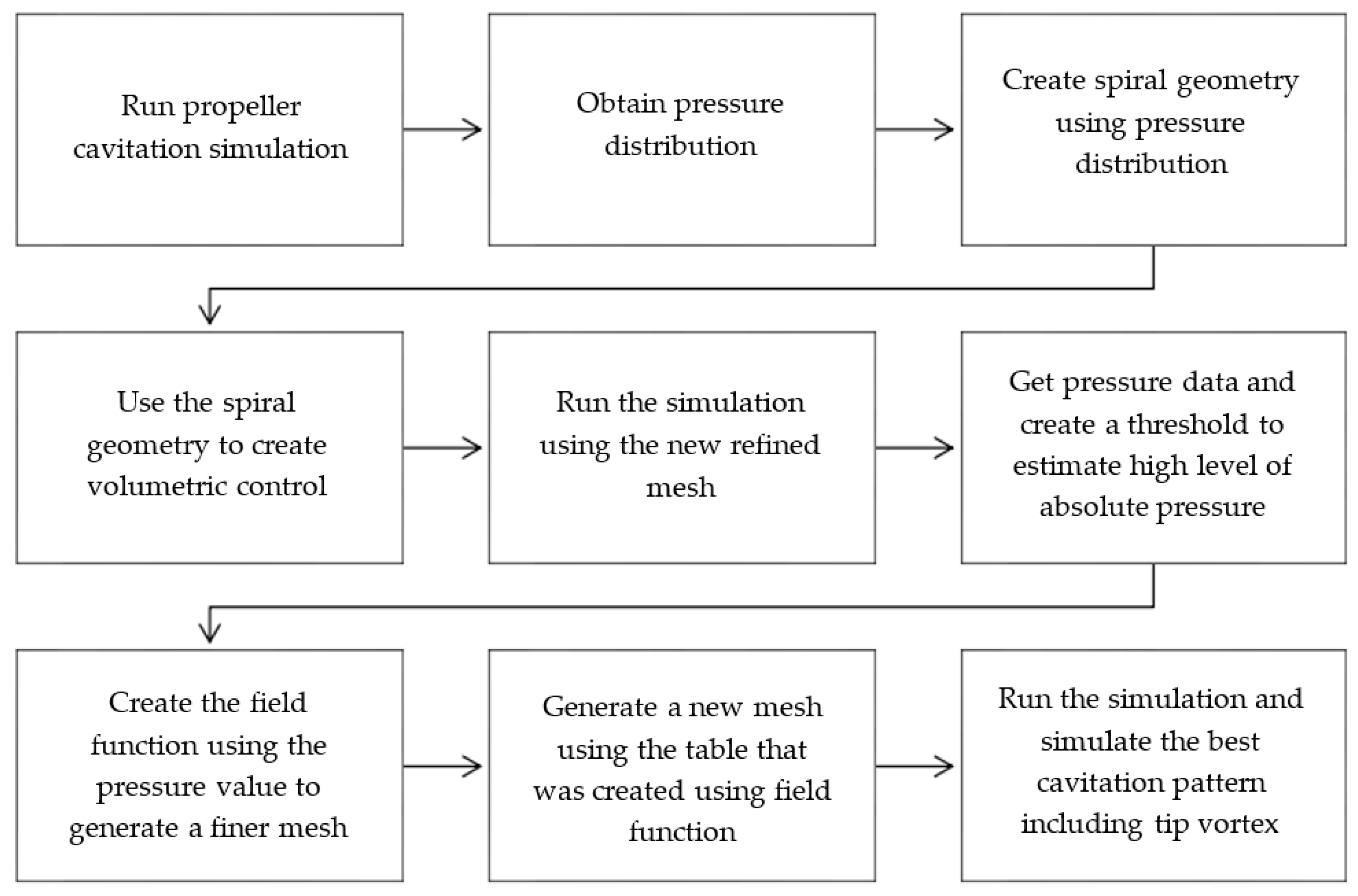
The mesh refinement technique from Step 4 to Step 6 has numerous advantages because the thresholds of scalars are easy to construct and export. Consequently, volumetric refinements mesh efficiently in parallel, and the resulting mesh is of good quality, since volumetric growth rates can be utilized. The computational procedures can be illustrated with a flowchart, as shown in Figure 4.

Figure 4.
The computational procedures adopted in the current study.
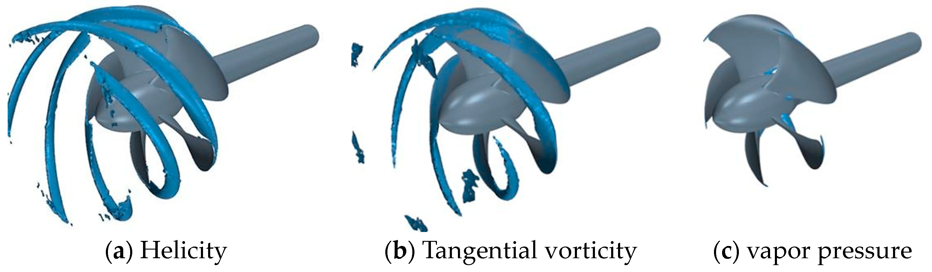
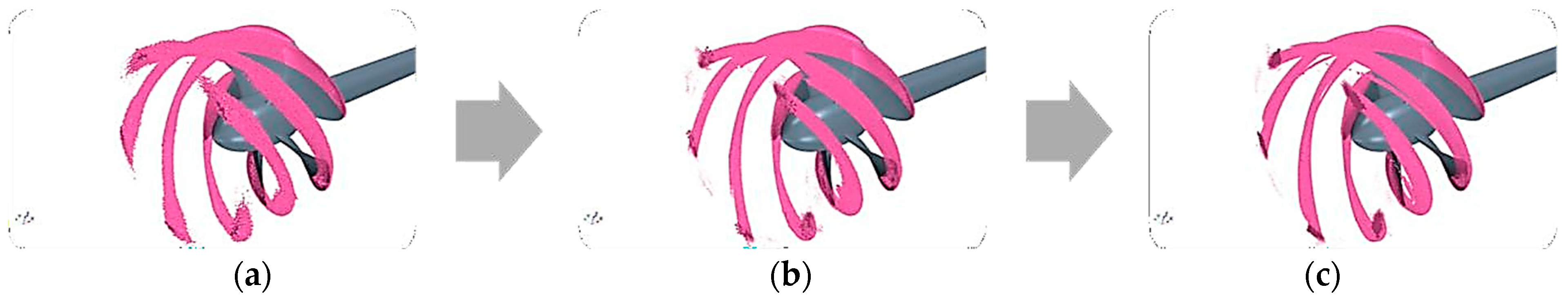
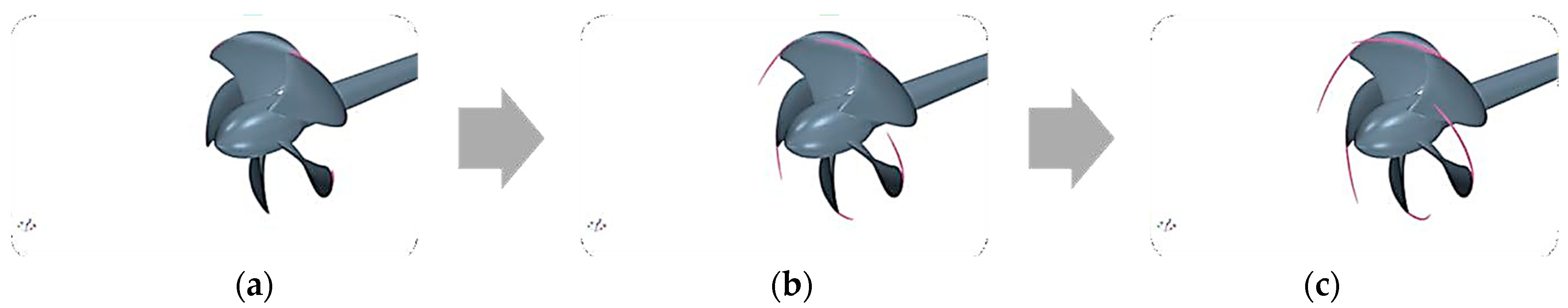
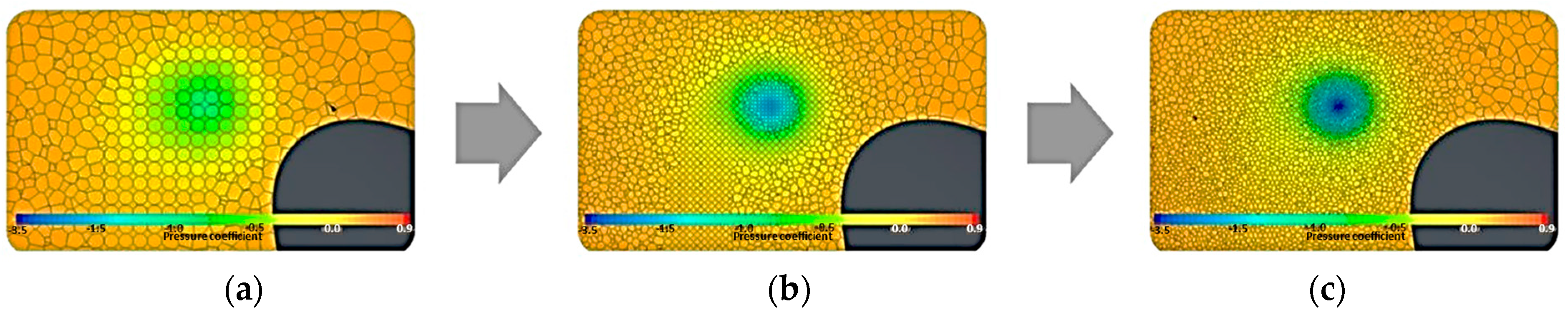
Once the initial solution had been run on the initial coarse mesh, multiple field functions were assessed to determine which could effectively delineate the tip vortex region and which threshold values should be used. To ensure that the refinements would only be applied to the blade tip, the field functions were filtered so they were only defined within the region satisfying 0.8 1.1. The field functions assessed were the helicity, tangential vorticity, and absolute pressure, which are shown in Figure 5. From the assessment, it was decided that a two-tier refinement strategy would be employed, with refinements applied to the region with a tangential vorticity > 300 s−1 and a finer refinement applied to the region with a vapor pressure (P) < 2771 Pa. The sizes of the volumetric refinement cells were reduced by 25% in each iteration (i.e., D/320, D/640, and D/960 for two, four, and six iterations, respectively). The volumetric refinements for iterations two, four, and six are shown in Figure 6 and Figure 7. As the mesh was refined, the absolute pressure in the region of volumetric refinement grew, indicating that the tip vortex was being resolved further downstream. Figure 8 shows the pressure coefficient and the mesh within the tip vortex, just downstream of the blade. It was observed that the vortex core pressure decreased as the mesh was refined; i.e., the tip vortex was better resolved.
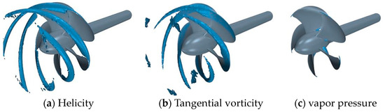
Figure 5.
Thresholds of the assessed field functions: (a) 1000 m/s2, (b) 300 s−1, (c) vapor pressure.

Figure 6.
Volumetric threshold refinements of tangential vorticity for iterations (a) two, (b) four, and (c) six.

Figure 7.
Volumetric threshold refinements of absolute pressure for iterations (a) two, (b) four, and (c) six.
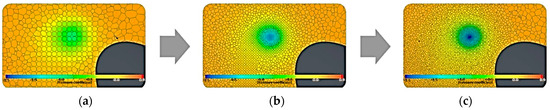
Figure 8.
The refined mesh and pressure coefficient within the tip vortex for iterations (a) two, (b) four, and (c) six.
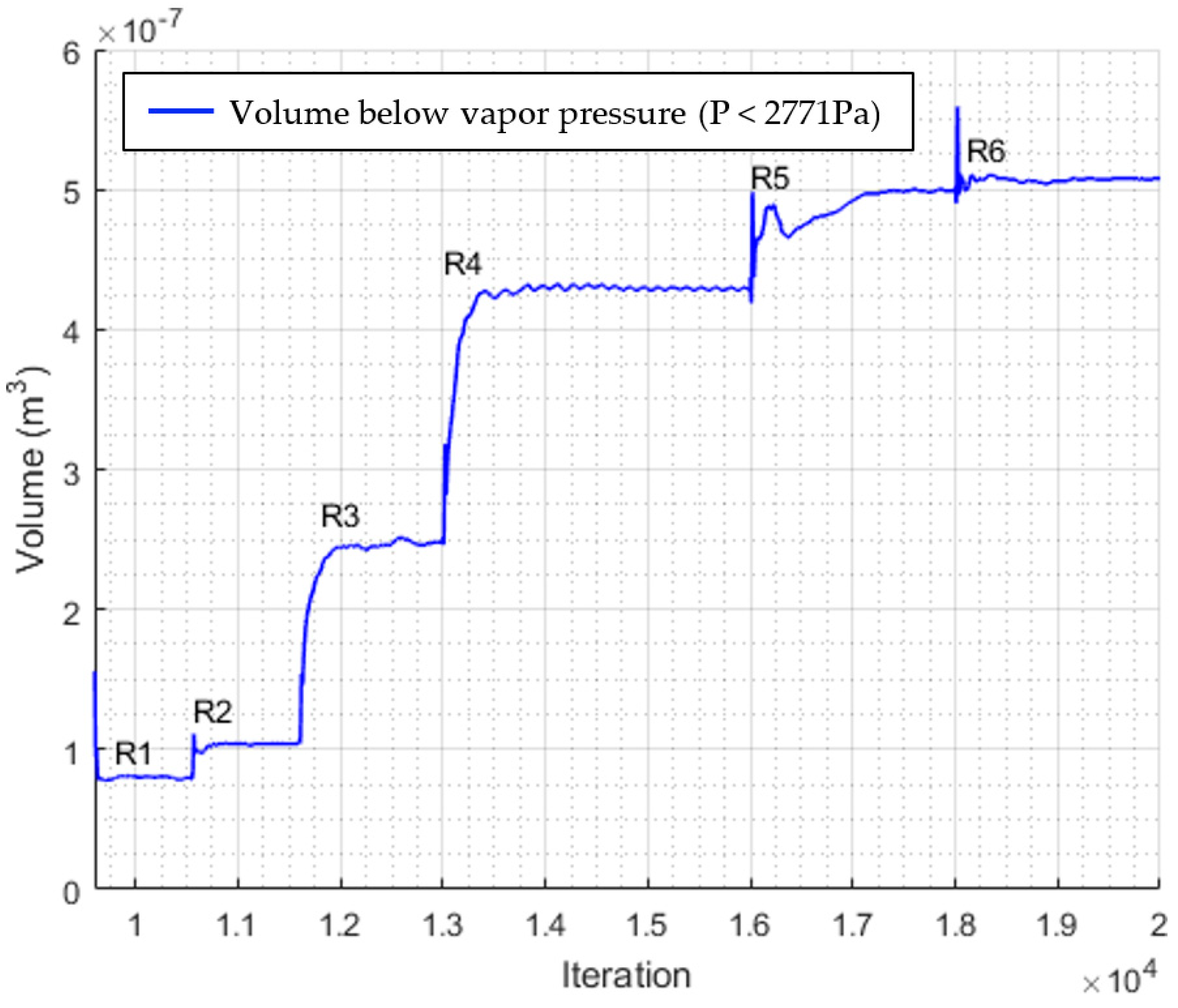
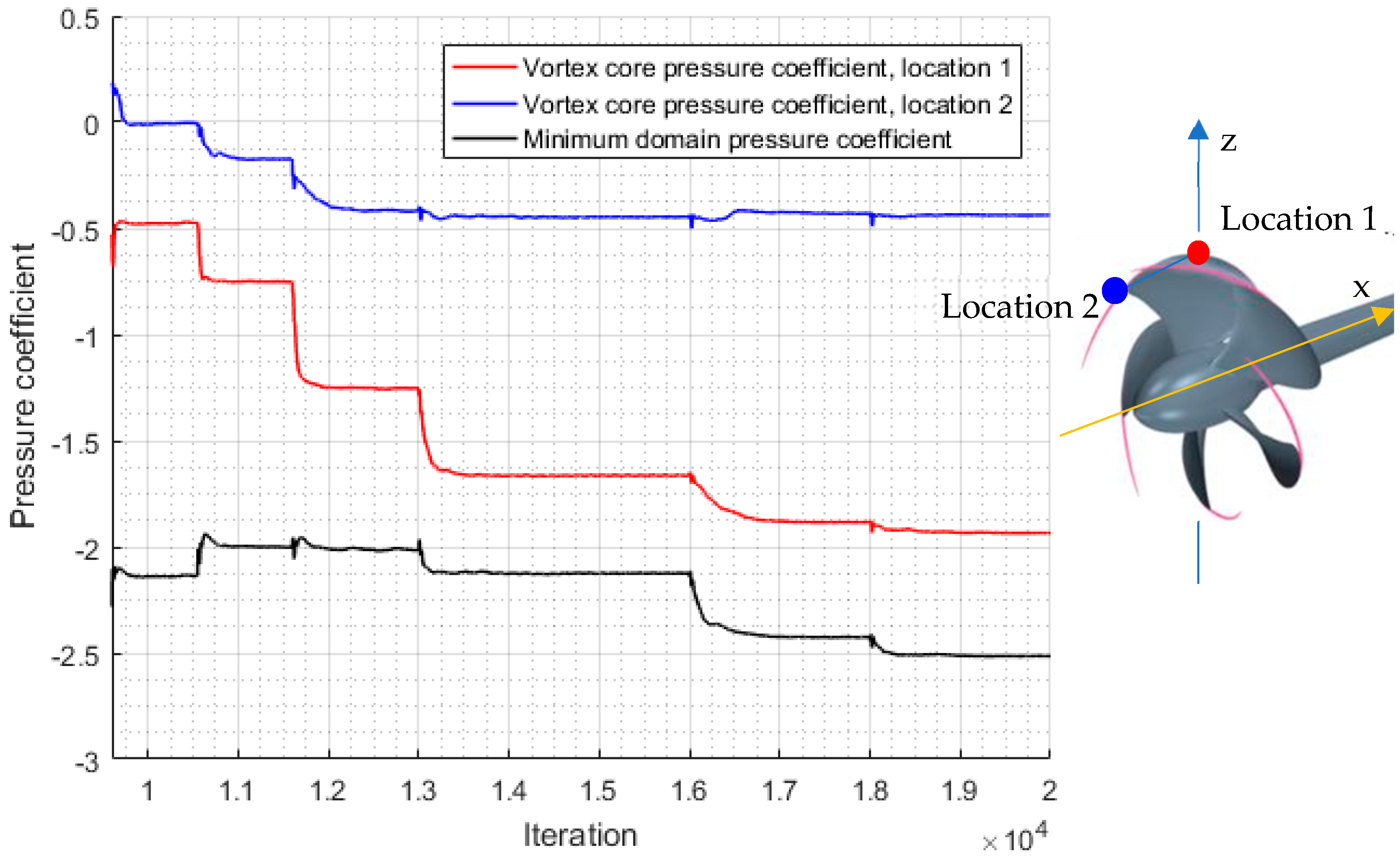
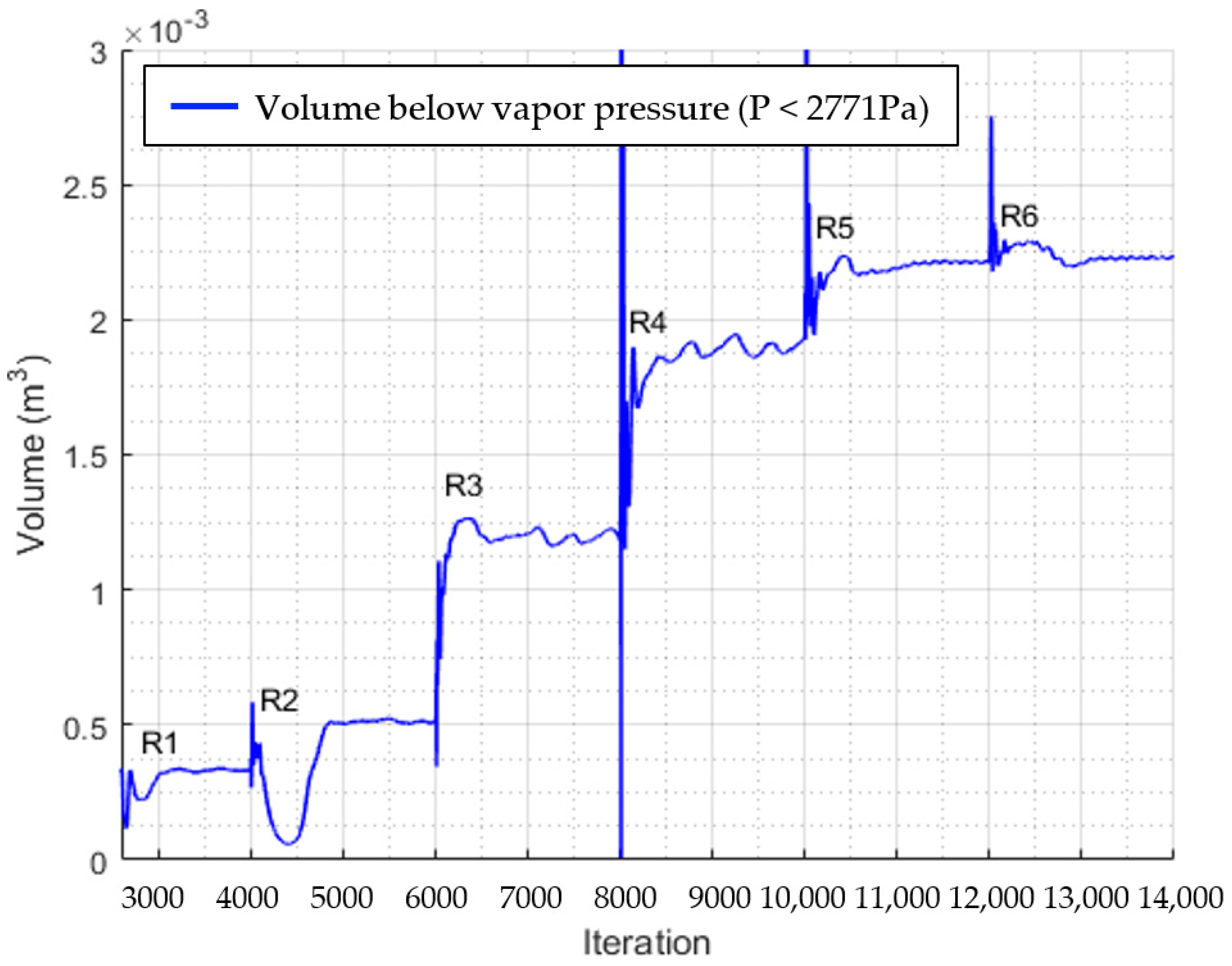
Figure 9 shows the convergence of the total volume of cells below the vapor pressure threshold throughout the refinement process. Annotations R1 to R6 denote the mesh refinement iterations. Figure 10 shows the vortex core pressure coefficient at two locations downstream of the propeller and the minimum pressure coefficient within the vortex (Cpmin). Vortex monitoring locations 1 and 2 were on the plane that intersected the propeller center line and were parallel to the x- and z-axes, with vortex location 2 occurring one full propeller tip vortex rotation downstream. As seen in Figure 9, convergence of the volume below the vapor pressure threshold was achieved by the fifth tip vortex mesh refinement (R5). Figure 10 shows that convergence was achieved for the vortex core pressure coefficients at locations 1 and 2.
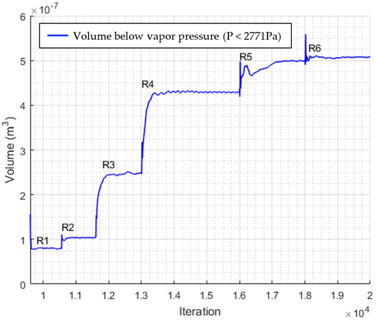
Figure 9.
Volume below the vapor pressure threshold for the small-scale propeller.
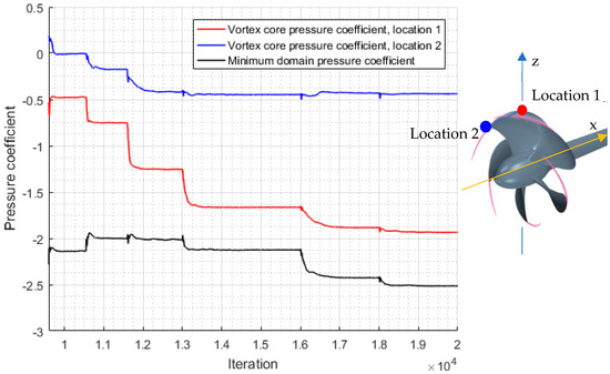
Figure 10.
The vortex core pressure coefficients at two locations downstream of the blade and the minimum domain (Cp) using the coarse process.
2.3. Validation
Numerical models need to be validated by comparing them with experimental data. Then, these numerical models can be used for further study. The open-water characteristics and cavitation phenomena of controllable pitch propeller VP1304 were measured in cavitation tunnel K15A of the Potsdam Model Basin [25]. A thrust coefficient (KT) of 0.2450 was obtained for the non-cavitating open-water case, while the computational KT value was 0.2458 for the finer mesh. The relative difference between the experimental test and the computation was 0.33%. These values met the requirements of numerical simulation. The computational wake pattern, including the complex roll-up phenomenon, was within acceptable limits. The numerical results show that the mesh refinement technique proposed in this paper could successfully simulate the extension of TVC and the roll-up phenomenon of TVC in the propeller wake. While monitoring KT throughout the refinements, it was observed that the tip vortex refinements did not have a significant impact.
3. Application of Mesh Refinement Process to Scaled-Up Propellers
The refinement process was applied to two scaled-up PPTC cases comprising medium- and full-scale propellers. The propeller diameter was scaled up by factors of six and fifteen to yield the medium- and full-scale propeller diameters, respectively. The simulation conditions were obtained by ensuring the similarity of the Reynolds number and advance ratio, as shown in Table 2. The fluid properties of the two larger propellers were representative of seawater at 15 degrees.
Table 2.
Scaled-up propeller dimensions and flow conditions.
It was found that the tangential vorticity threshold value could be non-dimensionalized using the propeller diameter and inlet velocity while maintaining the same relative refinement volume at all scales. A normalized tangential vorticity threshold value of 9.5 was employed in all cases. The absolute pressure threshold remained the same for all cases, as the fluid vapor pressure was assumed to be unchanged. Figure 11 and Figure 12 show the monitored values throughout the refinement process for the full-scale propeller.
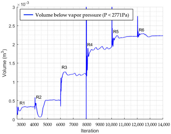
Figure 11.
Volume below the vapor pressure threshold for the full-scale propeller.
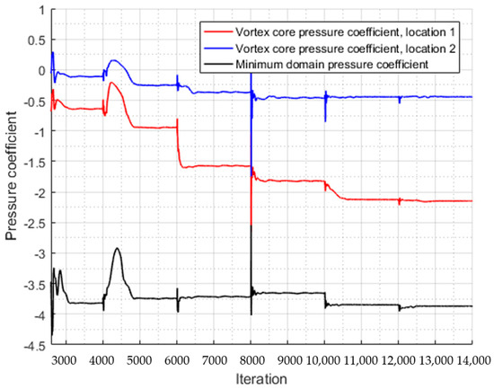
Figure 12.
The vortex core pressure coefficients at two locations downstream of the blade and the minimum domain (Cp) determined using the refinement process.
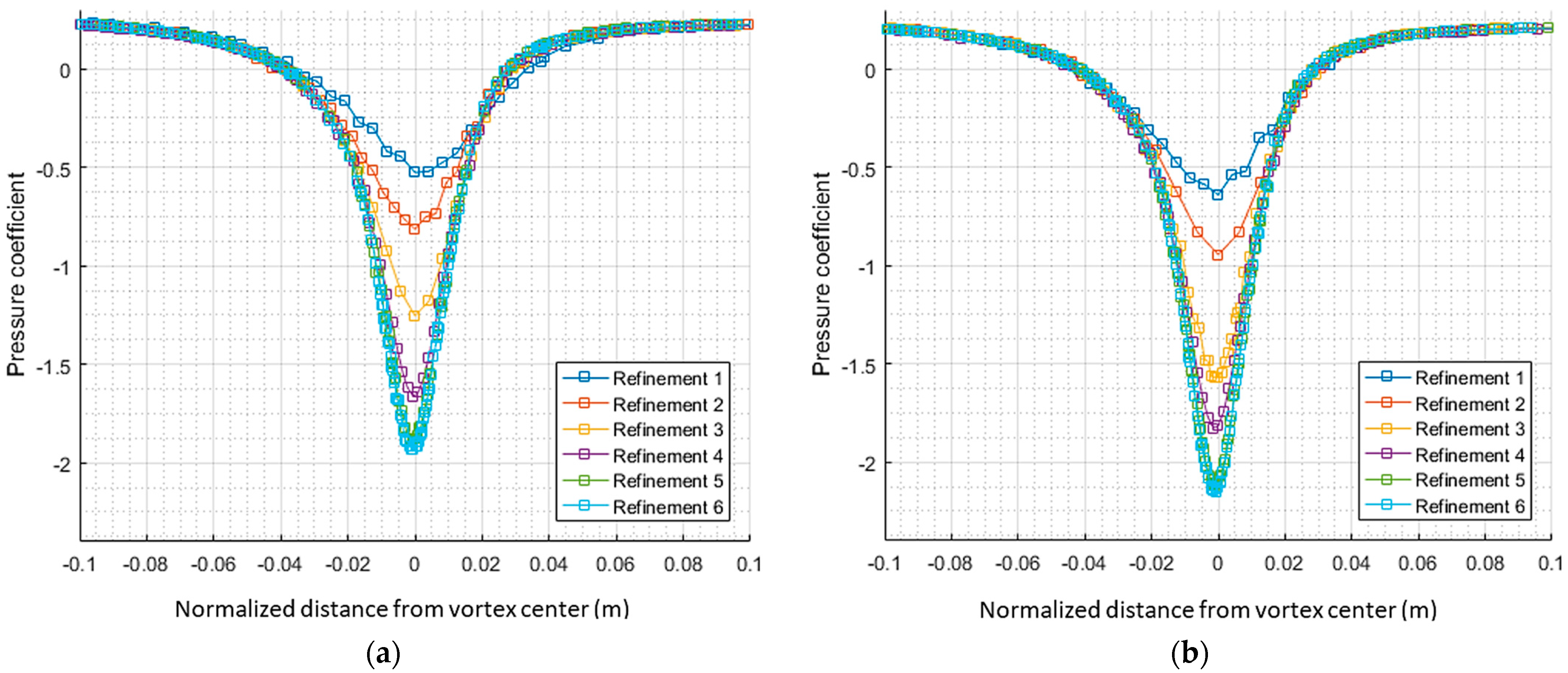
The convergence behavior remained more or less unchanged compared with the model-scale convergence, as shown in Figure 9 and Figure 10; however, it can be seen that the converged pressure coefficient values were lower for the full-scale propeller. To further investigate these differences, the pressure coefficient was plotted through the tip vortex at location 1 for both the scaled model and the full-scale propellers, as revealed in Figure 13. The distance from the center of the vortex was normalized using the propeller diameter in each case.
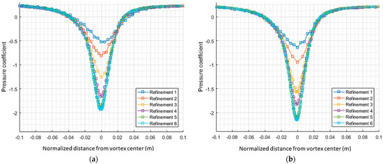
Figure 13.
A plot of Cp across the vortex core for (a) the scaled model and (b) the full-scale model.
These figures show that the vortex core pressures converged by R6, as there was very little change between the R5 and R6 mesh plots. It was observed that the free-stream pressure coefficient was the same in both cases, which was expected, as both were run with the same cavitation number and the relative size of the vortex core remained the same. It can be seen in Figure 12 that the minimum pressure coefficient was lower for the full-scale propeller.
4. Cavitation Inception Scaling
As the refinement process was applied to different propeller scales, a cavitation inception scaling law could be investigated. Assuming the cavitation inception number (σi) is −Cpmin, a scaling law can be defined according to Equation (1) [7].
where σi,1, Re1, and Cpmin,1 and σi,2, Re2, and Cpmin,2 are the cavitation numbers, Reynolds numbers, and minimum pressure coefficients of the model-scale and full-scale propellers, respectively, while γ is a scaling parameter. The cavitation number (σi) and the Reynolds number are defined in Equation (2) and Equation (3), respectively, where ρ is the water density; p is the reference pressure; pv is the vapor pressure; n is the revolution rate of the propeller; D is the diameter of the propeller; U∞ is the velocity of upstream; ν is the kinematic viscosity of water; and c0.7 is the chord length at r/R = 0.7. Note that the pressure coefficient is defined in Equation (4).
Many studies investigating the use of the appropriate scaling parameter (γ) have been reported, and they can be compared with the results obtained using the refinement process. The classic constant for γ was calculated by McCormick for a hydrofoil tip vortex and was found to be 0.4 [28]. However, recent studies have shown that this value is only applicable to the laminar flow regime and that γ should increase with the Reynolds number [7]. The equation for γ based on the turbulent boundary layer theory is shown in Equation (5), which is dependent on Re [7].
Table 3 shows the Re and tip vortex (Cpmin) values obtained from the refinement process for the three propeller scales. Table 4 shows the γ values obtained from the refinement process and from Equation (5).
Table 3.
Re and tip vortex (Cpmin) values for the three propeller scales.
Table 4.
Comparison between the scaling law obtained using CFD and Shen’s scaling law (Equation (5)).
It can be seen that the values obtained from the refinement process were much lower than the classic value of 0.4, as the flow within the propeller tip vortex in this Re range was highly turbulent. The γ values obtained from the refinement process were also lower than those predicted by Equation (2). However, the trend was the same, indicating that the refinement process results captured the Re dependency of the scaling law. Hsiao et al. [6] performed a CFD study on small, medium, and large propellers, representing Re numbers of 2.09 × 10⁶, 4.19 × 10⁶, and 8.38 × 10⁶, respectively, using both RANS and DNS (Direct Numerical Simulation) approaches. γ values of 0.33 and 0.15 were obtained for moving from small to medium scales and from medium to large scales, respectively, using RANS. The DNS approach yielded lower Cpmin values, and γ values of 0.22 and 0.11 were obtained. These results also displayed a general trend for γ to decrease as Re increased. As the simulations of the refinement process were performed at larger Re values, the values obtained using the refinement process were not unreasonable when compared with the higher Re scaling values of 0.15 (RANS) and 0.11 (DNS) obtained by Hsiao et al. It must be noted that only single-phase simulations were run in this study, and there is evidence that γ can be adjusted closer to the classic value of 0.4 when nuclei effects are modeled, provided that a statistical cavitation inception criterion is used and is not too stringent [6].
This study introduces an alternative approach to cavitation inception scaling using Computational Fluid Dynamics (CFD). By employing a mesh refinement process in CFD simulations, we can capture the minimum pressure coefficient (Cpmin) at the vortex core across different propeller scales. This allows for the derivation of a scaling law that is adaptable to various flow regimes and propeller sizes. The scaling law for cavitation inception can be defined as:
Using CFD-based simulations, the scaling parameter is determined based on the Reynolds number and the minimum pressure coefficient. Our findings indicate that as the Reynolds number increases, the value of γ decreases, diverging from McCormick’s classic value of 0.4, particularly in turbulent-flow regimes. For instance, the scaling parameter derived from the mesh refinement process was found to be significantly lower, consistent with recent research that incorporates turbulent boundary layer theory.
Table 3 presents the Reynolds numbers and Cpmin values obtained for the model, medium, and full-scale propellers using the CFD refinement process. The γ values computed using these data are shown in Table 4 and compared against Shen’s scaling law. The results from the CFD simulations highlight a decreasing trend in γ with the increasing Reynolds number, aligning with trends observed in recent analytical and numerical studies.
The key advantage of the CFD-based scaling approach lies in its flexibility and adaptability. Unlike traditional experimental scaling laws, which may not fully capture the complexity of real-world cavitation phenomena at larger scales, the CFD-based method can account for a broader range of flow conditions, including those with high turbulence or complex geometries. Moreover, the CFD refinement process provides detailed insights into the pressure distribution and vortex dynamics, which are difficult to measure experimentally, particularly in full-scale applications.
5. Conclusions
This study successfully developed and validated a mesh refinement process for predicting tip vortex cavitation (TVC) using the commercial CFD package STAR-CCM+. The refined mesh process demonstrated its ability to accurately capture the minimum pressure within a vortex core and effectively simulate TVC for different propeller scales. Based on the results of this study, the following conclusions can be drawn:
- The process achieved acceptable agreement with the experimental data, validating the numerical model in non-cavitation conditions.
- The mesh refinement process is applicable to both model-scale and full-scale propellers, maintaining consistency in relative refinement volume and convergence behavior.
- The converged Cpmin values obtained using the refinement process were gradually reduced when the scale and the Re values were increased, which allowed for the cavitation inception scaling parameter (γ) to be predicted. The scaling parameter obtained from the refinement process grew smaller with increasing Re values, which was in line with recent analytical and numerical studies.
Some limitations persist in CFD-based scaling, particularly in accurately modeling nuclei effects and unsteady flow interactions, which can significantly influence cavitation inception. While the results presented in this study demonstrate the effectiveness of CFD in capturing tip vortex cavitation behavior, further research is necessary to refine the turbulence models and incorporate multi-phase flow simulations to improve the accuracy of scaling predictions.
Author Contributions
Conceptualization, L.H.T.H., D.T.T. and D.D.T.; methodology, L.H.T.H. and D.T.T.; software, D.T.T. and D.D.T.; validation, L.H.T.H. and D.T.T.; formal analysis, D.T.T. and D.D.T.; investigation, L.H.T.H. and D.T.T.; resources, L.H.T.H. and D.D.T.; data curation, L.H.T.H. and D.T.T.; writing—original draft preparation, L.H.T.H. and D.T.T.; writing—review and editing, L.H.T.H. and D.D.T.; visualization, D.T.T.; supervision, L.H.T.H.; project administration, L.H.T.H. and D.D.T.; funding acquisition, L.H.T.H. All authors have read and agreed to the published version of the manuscript.
Funding
This research was funded by the Ministry of Education and Training, Vietnam (Grant No. B2022-TSN-06).
Data Availability Statement
The original contributions presented in this study are included in the article. Further inquiries can be directed to the corresponding author.
Conflicts of Interest
The authors declare no conflicts of interest.
References
- Bhattacharyya, A.; Krasilnikov, V.; Steen, S. A CFD-based scaling approach for ducted propellers. Ocean Eng. 2016, 123, 116–130. [Google Scholar] [CrossRef]
- Mitra, A.; Panda, J.P.; Warrior, H.V. The effects of free stream turbulence on the hydrodynamic characteristics of an AUV hull form. Ocean Eng. 2019, 174, 148–158. [Google Scholar] [CrossRef]
- Panda, J.P.; Handique, J.; Warrior, H.V. Mechanics of drag reduction of an axisymmetric body of revolution with shallow dimples. Proc. Inst. Mech. Eng. Part M J. Eng. Marit. Environ. 2023, 237, 227–237. [Google Scholar] [CrossRef]
- Jagadale, S.L.; Bhattacharyya, A.; Nagarajan, V.; Sha, O.P.; Kumar, C.S. Hydrodynamic characteristics of an Asian sea bass-inspired underwater body. Appl. Ocean Res. 2023, 141, 103794. [Google Scholar] [CrossRef]
- Mitra, A.; Panda, J.; Warrior, H. The hydrodynamic characteristics of autonomous underwater vehicles in rotating flow fields. Proc. Inst. Mech. Eng. Part M J. Eng. Marit. Environ. 2023, 238, 691–703. [Google Scholar] [CrossRef]
- Hsiao, C.-T.; Chahine, G.L. Scaling of tip vortex cavitation inception for a marine open propeller. In Proceedings of the 27th Symposium on Naval Hydrodynamics, Seoul, Republic of Korea, 5–10 October 2008. [Google Scholar]
- Shen, Y.T.; Gowing, S.; Jessup, S. Tip vortex cavitation inception scaling for high reynolds number applications. J. Fluids Eng. 2009, 131, 071301. [Google Scholar] [CrossRef]
- Szantyr, J.A.; Flaszynski, P.; Tesch, K.; Suchecki, W.; Alabrudzinski, S. An experimental and numerical study of tip vortex cavitation. Pol. Marit. Res. 2011, 18, 14–22. [Google Scholar] [CrossRef]
- Fujiyama, K.; Kim, C.-H.; Hitomi, D. Performance and cavitation evaluation of marine propeller using numerical simulations. In Proceedings of the Second International Symposium on Marine Propulsors (smp’11), Hamburg, Germany, 15–17 June 2011. [Google Scholar]
- Yilmaz, N.; Khorasanchi, M.; Altar, M. An investigation into computational modelling of cavitation in a propeller’s slipstream. In Proceedings of the Fifth International Symposium on Marine Propulsion (smp’17), Espoo, Finland, 12—15 June 2017. [Google Scholar]
- Usta, O.; Korkut, E. A study for cavitating flow analysis using DES model. Ocean Eng. 2018, 160, 397–411. [Google Scholar] [CrossRef]
- Gaggero, S.; Tani, G.; Viviani, M.; Conti, F. A study on the numerical prediction of propellers cavitating tip vortex. Ocean Eng. 2014, 9, 137–161. [Google Scholar] [CrossRef]
- Zhao, M.; Zhao, W.; Wan, D. Numerical simulations of propeller cavitation flows based on OpenFOAM. J. Hydrodyn. 2020, 32, 1071–1079. [Google Scholar] [CrossRef]
- Usta, O.; Korkut, E. Prediction of cavitation development and cavitation erosion on hydrofoils and propellers by Detached Eddy Simulation. Ocean Eng. 2019, 191, 106512. [Google Scholar] [CrossRef]
- Asnaghi, A.; Svennberg, U.; Bensow, R.E. Analysis of tip vortex inception prediction methods. Ocean Eng. 2018, 167, 187–203. [Google Scholar] [CrossRef]
- Asnaghi, A.; Svennberg, U.; Bensow, R.E. Large Eddy Simulations of cavitating tip vortex flows. Ocean Eng. 2020, 195, 106703. [Google Scholar] [CrossRef]
- Yilmaz, N.; Aktas, B.; Atlar, M.; Fitzsimmons, P.A.; Felli, M. An experimental and numerical investigation of propeller-rudder-hull interaction in the presence of tip vortex cavitation (TVC). Ocean Eng. 2020, 216, 10802. [Google Scholar] [CrossRef]
- Gao, H.; Zhu, W.; Liu, Y.; Yan, Y. Effect of various winglets on the performance of marine propeller. Appl. Ocean Res. 2019, 86, 246–256. [Google Scholar] [CrossRef]
- Blazek, J. Computational Fluid Dynamics_Principles and Applications, 2nd ed.; Elsevier: Amsterdam, The Netherlands, 2006. [Google Scholar]
- Pope, S.B. Turbulent Flows. Measurement Science and Technology; Cambridge: Cambridge, UK, 2001; Volume 12, pp. 2020–2021. [Google Scholar]
- Saugaut, P. Large Eddy Simulation for Incompressible Flows; Springer: Berlin/Heidelberg, Germany, 2006. [Google Scholar]
- Sipilä, T.; Siikonen, T. RANS predictions of a cavitating tip vortex. In Proceedings of the CAV 2012: Eight International Symposium on Cavitation, Singapore, 13–16 August 2012. [Google Scholar]
- Sipilä, T.; Sánchez-Caja, A.; Siikonen, T. Eddy vorticity in cavitating tip vortices modelled by different turbulence models using the RANS approach. In Proceedings of the 11th World Congress on Computational Mechanics, WCCM 2014, 5th European Conference on Computational Mechanics, ECCM 2014 and 6th European Conference on Computational Fluid Dynamics, ECFD, Barcelona, Spain, 20–25 July 2014. [Google Scholar]
- Viitanen, V.; Siikonen, T. Numerical simulation of cavitating marine propeller flows. In Proceedings of the MekIT17—9th National Conference on Computational Mechanics, Trondheim, Norway, 11–12 May 2017. [Google Scholar]
- Heinke, H.J. Potsdam Propeller Test Case (PPTC) Cavitation Tests with the Model Propeller VP1304; Report 3753; Schiffbau-Versuchsanstalt: Potsdam, Germany, 2011. [Google Scholar]
- ITTC. Practical guidelines for ship CFD applications. In Recommended Procedure and Guidelines; ITTC: Zurich, Switzerland, 2011. [Google Scholar]
- Yilmaz, N.; Atlar, M.; Khorasanchi, M. An improved Mesh Adaption and Refinement approach to Cavitation Simulation (MARCS) of propellers. Ocean Eng. 2019, 171, 139–150. [Google Scholar] [CrossRef]
- McCormick, B.W. On cavitation produced by a vortex trailing from a lifting surface. ASME J. Basic Eng. 1962, 84, 369–379. [Google Scholar] [CrossRef]


Disclaimer/Publisher’s Note: The statements, opinions and data contained in all publications are solely those of the individual author(s) and contributor(s) and not of MDPI and/or the editor(s). MDPI and/or the editor(s) disclaim responsibility for any injury to people or property resulting from any ideas, methods, instructions or products referred to in the content. |
© 2024 by the authors. Licensee MDPI, Basel, Switzerland. This article is an open access article distributed under the terms and conditions of the Creative Commons Attribution (CC BY) license (https://creativecommons.org/licenses/by/4.0/).