Development and Validation of a Compressible Reacting Gas-Dynamic Flow Solver for Supersonic Combustion

Abstract

An approach based on the OpenFOAM library has been developed to solve a high-speed, multicomponent mixture of a reacting, compressible flow. This work presents comprehensive validation of the newly developed solver, called compressibleCentralReactingFoam, with different supersonic flows, including shocks, expansion waves, and turbulence–combustion interaction. The comparisons of the simulation results with experimental and computational data confirm the fidelity of this solver for problems involving multicomponent high-speed reactive flows. The gas dynamics of turbulence–chemistry interaction are modeled using a partially stirred reactor formulation and provide promising results to better understand the complex physics involved in supersonic combustors. A time-scale analysis based on local Damköhler numbers reveals different regimes of turbulent combustion. In the core of the jet flow, the Damköhler number is relatively high, indicating that the reaction time scale is smaller than the turbulent mixing time scale. This means that the combustion is controlled by turbulent mixing. In the shear layer, where the heat release rate and the scalar dissipation rate have the highest value, the flame is stabilized due to finite rate chemistry with small Damköhler numbers and a limited fraction of fine structure. This solver allows three-dimensional gas dynamic simulation of high-speed multicomponent reactive flows relevant to practical combustion applications.

1. Introduction

The supersonic airbreathing or supersonic combustion ramjet (scramjet) engine is the most promising technology for significant reduction of flight times for long-distance civilian flights and the first stages of space systems for putting payloads into orbit. The future of access-to-space systems is faced with many technical and economic challenges. Designing and testing scramjet systems requires the ability to adequately understand and control the complex flow physics of these systems. The high-speed flow in the propulsion systems leads to many difficulties in achieving and maintaining combustion [1,2]. One of the significant features of the scramjet is that the supersonic flow conditions in the combustor lead to very short residence times for fuel and air, typically of the order of milliseconds; therefore, the fuel must mix with the supersonic air flow and burn entirely within a short time. Thus, future hypersonic propulsion systems’ success will largely depend on efficient injection, mixing, and combustion processes inside the supersonic combustion chamber [1,3].

Computational fluid dynamics (CFD) and experimental testing have seen significant advances through the years in terms of reliability and accuracy. However, in the case of supersonic and hypersonic regimes, realistic high-enthalpy conditions can only be maintained and thus measured in experimental facilities for a very short period, on the order of milliseconds [4], which is insufficient to provide a comprehensive analysis for designing efficient scramjet engines. A numerical approach remains the primary analysis tool to cover the operating regimes of a scramjet consistently. CFD methods targeting the solution of the flow field inside supersonic engines are faced with the challenges of addressing internal flow dominated by complex shock wave patterns, shock wave boundary layer interaction with its separation, and most importantly, supersonic turbulence–combustion interaction, which, in many cases, is characterized by finite rate chemistry. Inaccurate prediction of shock position and separation locations within the engine can lead to unreliable results when reactions are activated, risking the success of the entire design process.

The computational approaches to simulate turbulent flows by solving the compressible Navier–Stokes equations are Direct Numerical Simulation (DNS), Large Eddy Simulation (LES), and Reynolds Averaged Navier–Stokes (RANS). RANS is very useful in many real-world industrial applications, as these simulations are computationally less expensive than DNS and LES. In RANS, fewer equations must be solved, and they can be solved with limited computational resources. However, because the turbulent flows using RANS are not fully resolved, turbulence–combustion interactions are also unresolved. Moreover, the reacting flow is highly nonlinear, unstable, and non-stationary. RANS will not adequately model turbulence–combustion interactions in a scramjet [5] due to these constraints. Direct Numerical Simulation (DNS) is a detailed computational approach that demands a fine grid to resolve all turbulent length scales and small time-steps comparable to chemical time scales. Hence, DNS requires tremendous computational resources for the simulations of the high-speed flows of practical interest. On the other hand, Large-Eddy Simulation (LES) resolves large scales of the turbulent flow, i.e., turbulent eddies larger than the smallest mesh size, while the smallest scales are modeled [6,7,8]. Thus, this feature of LES leads to a significant reduction in computational resources compared to DNS. During the past decade, LES, which is a compromise between the DNS [9] and the RANS [10] methods, has been extensively used to study high-speed combustion applications [11,12,13]. In LES, turbulence scales larger than the grid spacing are resolved, while subgrid scales and their effects on the large scales are modeled [14]. LES has been shown [15,16,17,18,19] to be computationally practical for modeling unsteady phenomena, including transient combustion events. One of the critical aspects of modeling unsteady turbulent combustion in high-speed jets is appropriately accounting for the influence of turbulence on the rate of chemical reactions. Transient turbulent combustion will also depend on accurately modeling the interaction between the jet mixing layer and the surrounding air.

DNS and LES of compressible turbulent reactive flows require highly accurate numerical schemes, which must capture shock waves, describe multicomponent mixtures and detailed chemical kinetics, and resolve a broad range of length scales. Combustion processes involve highly nonlinear chemical reactions and many species. Numerical simulation of combustion in supersonic flow fundamentally differs from combustion in the subsonic regime. In supersonic combustion, chemical reactions occur under conditions of high pressure, temperature, and density. These conditions can significantly alter chemical kinetics and reaction rates, leading to different reaction pathways and species formation compared to subsonic conditions. Ignition and flame stabilization processes in supersonic combustion devices may differ significantly from those observed in the subsonic regime [3]. Furthermore, turbulence increases the mixing of fuel and oxidizer and enhances combustion [20]. In turn, the combustion can intensify the turbulence via flow expansion [20]. As a result, the turbulent fluctuations can be very large [21].

Various CFD solvers in the literature are used to simulate high-speed airbreathing engines. These codes can be broadly categorized into three main categories: commercial, open-source, and in-house solvers, each with its own advantages and disadvantages. The commercial codes such as Fluent [22], StarCCM++ [23], NASA codes REACTMB [24], WIND-US [25], TAU-code code [26], VULCAN [27], and SU2 [28] have been used successfully in solving the above-mentioned problems. Commercial solvers can be expensive, with limited access to the source code. Open-source solvers are typically freely available, with access to the source code, allowing for extensive customization and the development of user-specific models or algorithms. The open-source community often collaborates on code development. Among the open-source codes, the OpenFOAM library is a well-established open platform in the scientific community [29]. It is noteworthy that there are several in-house codes reported in the literature for high-speed compressible reacting flows [13,14,30,31,32,33,34,35,36,37]. These codes have been used to solve many problems involving turbulence–combustion interactions. Some of them are built on the OpenFOAM foundation. However, none of these codes are readily and freely available, i.e., they are not yet fully open-source [38].

The OpenFOAM library has high-fidelity reactive flow solvers (e.g., reactingFoam) that were validated for a variety of turbulent combustion applications under subsonic conditions [10]. As this solver lacks appropriate model construction for high-speed flows, a density-based compressible flow solver, namely rhoCentralFoam, was developed for high-speed flow modeling based on the central-upwind schemes of Kurganov and Tadmor [39,40]. Greenshields et al. [41] detailed this solver and validation against standard test cases. The solver was validated for compressible gas flow, including shocks and wave expansion. However, the rhoCentralFoam is limited to non-reacting flows. Therefore, in the current work, an in-house code, compressibleCentralReactingFoam, was developed by combining rhoCentralFoam with reactingFoam in the latest version of the OpenFOAM (i.e., v2306 [42]), to simulate high-speed compressible multicomponent reactive flows.

The challenges of scramjet simulation are due to multiscale (in terms of space and time) phenomena of non-steady, non-equilibrium turbulent combustion in the supersonic flow. Thus, the model needs to account for complex mixing phenomena, non-equilibrium transfer of turbulence energy, and the interaction between turbulence and chemical kinetics. This paper demonstrates a physics-based methodology/computational tool, namely the compressibleCentralReactingFoam solver, to model the complex physical phenomena of reactive multicomponent gas flow at high Mach numbers. Moreover, the present work aims to quantitatively assess the accuracy and applicability of the newly developed solver in modeling supersonic combustion. A set of validation test cases are presented to demonstrate the capabilities of the solver, ranging from simple one-dimensional shock-tube problems to complex three-dimensional scramjet combustor. In addition, three popular subgrid models—Smagorinsky model (SMG) [43,44], the Localized Dynamic k-equation Model (LDkEqn) [45,46], and Wall Adapted Local Eddy-Viscosity (WALE) [47]—are evaluated for simulating supersonic turbulent combustion under conditions relevant to scramjet operation. Below, short descriptions of these models are provided. Section 2.1 presents the governing equations of supersonic multicomponent gas flow with chemical reactions. Subgrid flow equations and closure of the combustion model are discussed in Section 2.2 and Section 2.3, respectively. Section 2.4 briefly discusses the numerical method and algorithm of the compressibleCentralReactingFoam solver. In Section 3.1.1, validations of 1D shock tube problems are solved. Section 3.1.2 presents simulations of 3D problems showing comparisons with experiments. The validation of turbulence–combustion interactions in the model scramjet combustor is presented in Section 3.1.3. The influence of turbulence models on scramjet combustion and analysis of turbulent–combustion interaction are presented in Section 3.2 and Section 3.3, respectively. Section 4 presents conclusions.

2. Materials and Methods

2.1. Governing Equations

The governing equations of a reactive multicomponent mixture of gases consist of the continuity, the momentum, the energy balance, and the balance of mass fraction equations. A LES formulation is used to solve the equations for turbulent fluid flow. After Favre filtering, these equations can be written as [14,48]

$${\partial }_t\left(\overline{\rho }\right)+\mathsf{\nabla }·\left(\overline{\rho }\tilde{\mathit{u}}\right)=0,$$

(1)

$${\partial }_t\left(\overline{\rho }\tilde{\mathit{u}}\right)+\mathsf{\nabla }·\left(\overline{\rho }\tilde{\mathit{u}}⨂\tilde{\mathit{u}}\right)=-\mathsf{\nabla }\overline{p}+\mathsf{\nabla }·\left(\overline{\mathit{S}}-{\mathit{B}}^{SGS}\right),$$

(2)

$${\partial }_t\left(\overline{\rho }\tilde{E}\right)+\mathsf{\nabla }·\left(\overline{\rho }\tilde{\mathit{u}}\tilde{E}\right)=\mathsf{\nabla }·(-\overline{p}\tilde{\mathit{u}}+\overline{\mathit{S}}·\tilde{\mathit{u}}+\overline{\mathit{h}}-{\mathit{b}}_E^{SGS})+{\overline{\dot{\omega }}}_T,$$

(3)

$${\partial }_t\left({\overline{\rho }\tilde{Y}}_i\right)+\mathsf{\nabla }·\left({\overline{\rho }\tilde{\mathit{u}}\tilde{Y}}_i\right)=\mathsf{\nabla }·\left({\overline{\mathit{J}}}_i-{\mathit{b}}_i^{SGS}\right)+{\overline{\dot{\omega }}}_i,(i=1,\dots ,M-1)$$

(4)

Here, the symbol “~” denotes Favre-filtered quantities, and “$-$“ indicates filtered quantities; $\rho$ is the gas mixture density, $\mathit{u}$ is the velocity vector, $p$ is the pressure, $\mathit{S}$ is the viscous stress tensor, $E$ is the total energy, $\mathit{h}$ is the heat flux vector, ${\dot{\omega }}_T$ is combustion heat release, $Y_i$ is the specific mass fraction, ${\mathit{j}}_i$ is the diffusive flux, and $\dot{{\omega }_i}$ is the species reaction rate of $i^{th}$ species. M is a number of species, and due to the conservation ${\sum }_i{Y}_i=1$, the last species fraction is defined from this equation. The terms of subgrid flow physics in Equations (1)–(4) are denoted by SGS upper indexes. The pressure of the gas mixture is equal to

$$p=\rho {\mathcal{R}}_{u}T{\sum }_{i=1}^M(Y_i/W_i),$$

(5)

where ${\mathcal{R}}_u$ is the universal gas constant, $T$ is the temperature, and $W_i$ is the molar mass of $i^{th}$ species. The viscous stress tensor is defined as

$$\mathit{S}=2\mu {\mathit{D}}_D$$

(6)

where ${\mathit{D}}_D$ is the deviatoric part of the rate strain tensor and $\mu$ is the dynamic viscosity, which is modeled using Sutherland’s law

$$\mu =A_s\sqrt{T}/(1+T_s/T),$$

(7)

where $A_s,T_s$ are Sutherland’s coefficient and temperature [30]. The deviatoric part of the rate strain tensor is defined as

$${\mathit{D}}_D=\left(\mathsf{\nabla }\mathit{u}+\mathsf{\nabla }{\mathit{u}}^T\right)/2-\left(\mathsf{\nabla }·u\right)\mathit{I}/3$$

(8)

The total energy is defined as

$$E={\sum }_{i=1}^M{Y}_i{\int }_{T_0}^T{C}_{p,i}dT-p/\rho +(\mathit{u}·\mathit{u})/2$$

(9)

where $C_{p,i}$ is the heat capacity at constant pressure, which is defined from JANAF polynomials [49]. Following [2], one may postulate that the gas mixture behaves as a linear viscous fluid with Fourier heat conditions and Fickian species for diffusive flux, such as

$$\mathit{h}=\kappa \mathsf{\nabla }T$$

(10)

and

$${\mathit{j}}_i=D_i\mathsf{\nabla }{Y}_i$$

(11)

where $\kappa =\mu /Pr$ is the thermal diffusivity, $Pr$ is the Prandtl number, $D_i=\mu /S{c}_i$ is the species diffusivities, and $S{c}_i$ is the Schmidt number. The combustion heat release is defined as

$${\dot{\omega }}_T=\sum _{\mathit{i}\mathbf{=}\mathbf{1}}^M\left({\dot{\omega }}_i∆h_{f,i}^0\right)$$

(12)

where $∆h_{f,i}^0$ is the formation enthalpy of $i^{th}$ species. The reaction rate is defined as

$${\dot{\omega }}_i=W_i\sum _{j=1}^N{\omega }_{ij}^0$$

(13)

where ${\omega }_{ij}^0$ is the reaction rate of elementary reaction, and N > 1 when detailed chemical mechanism is used.

2.2. Subgrid Flow Equations

Subgrid pressure fluctuations and dissipation terms will be neglected. The subgrid flow physics is concealed in the subgrid stress tensor

$${\mathit{B}}^{SGS}=\overline{\rho }\left(\widetilde{\mathit{u}⨂\mathit{u}}-\tilde{\mathit{u}}⨂\tilde{\mathit{u}}\right)$$

(14)

and flux vectors

$${\mathit{b}}_i^{SGS}=\overline{\rho }\left(\widetilde{\mathit{u}{Y}_i}-\tilde{\mathit{u}}\widetilde{Y_i}\right),$$

(15)

$${\mathit{b}}_E^{SGS}=\overline{\rho }\left(\widetilde{\mathit{u}E}-\tilde{\mathit{u}}\tilde{E}\right)+\left(\widetilde{p\mathit{u}}-\overline{p}\tilde{\mathit{u}}\right)-(\widetilde{\mathit{S}·\mathit{u}}-\tilde{\mathit{S}}·\tilde{\mathit{u}}),$$

(16)

which results from filtering the nonlinear convective terms.

The LES Equations (1)–(4) are closed by providing submodels for ${\mathit{B}}^{SGS}$, ${\mathit{b}}_{\mathit{i}}^{SGS}$, ${\mathit{b}}_E^{SGS}$. The most common subgrid models used for high-speed reactive flows are a class of Smagorinsky models [43,44] of the form

$${\mathit{B}}^{SGS}=-2{\mu }_k{\tilde{\mathit{D}}}_D+(2/3)\overline{\rho }k\mathit{I},$$

(17)

where ${\mu }_k$ is the subgrid viscosity and $k$ is the subgrid kinetic energy,

$${\mathit{b}}_i^{SGS}=({\mu }_k/S{c}_t)\nabla {\tilde{Y}}_i,$$

(18)

and

$${\mathit{b}}_E^{SGS}=({\mu }_k/P{r}_{\mathrm{t}})\nabla \tilde{\mathrm{E}},$$

(19)

where $S{c}_t\approx 0.7$ and $P{r}_{\mathrm{t}}\approx 0.8$ are the turbulent Schmidt and Prandtl numbers, respectively. To close $k$ and ${\mu }_k$ in the Smagorinsky model (SMG) [44], they are formulated as

$${\mu }_k=c_D\overline{\rho }{∆}^2\left|\tilde{\mathit{D}}\right|$$

(20)

and

$$k=c_l{∆}^2{\left|\tilde{\mathit{D}}\right|}^2,$$

(21)

where $∆$ is the filter size, and $c_D$ and $c_l$ are model coefficients.

The second subgrid model used in this work is the Local Dynamic k-equation (LDkEqn) [45,46]. The LDkEqn turbulence model is an advanced subgrid-scale (SGS) turbulence model used in Large Eddy Simulation to improve the prediction of turbulent flows. Instead of using fixed model coefficient constants (as in the SMG), the LDkEqn model calculates them dynamically by adjusting the model coefficients to match the resolved flow characteristics. This adaptability allows the model to capture variations in turbulence intensity and anisotropy better. The LDkEqn model exhibits a scale-adaptive behavior, which means it can adapt to different turbulence scales in the flow. This adaptability is particularly beneficial in LES, where a wide range of turbulent structures exist; also, the LDkEqn model is designed to provide better predictions near walls. For the LDkEqn, a modeled transport equation

$${\partial }_t\left(\overline{\rho }k\right)+\nabla ·\left(\overline{\rho }k\tilde{\mathit{u}}\right)=-\mathit{B}·\tilde{\mathbf{D}}+\mathsf{\nabla }·\left({\mu }_k\mathsf{\nabla }k\right)-c_{\epsilon }\overline{\rho }{k}^{3/2}/∆$$

(22)

is solved for $k$, and subgrid viscosity is modeled as

$${\mu }_k=c_k\overline{\rho }∆k^{1/2}$$

(23)

The model coefficients $c_k$ and $c_{\epsilon }$ are evaluated dynamically using scale similarity.

The third subgrid model used in this work is the Wall Adapted Local Eddy-Viscosity (WALE) model [47]. The WALE model is designed to improve the accuracy of LES by providing a more accurate representation of the subgrid-scale turbulence in the near-wall region, where traditional SGS models may struggle to capture complex flow phenomena. The WALE model is specifically designed to address the near-wall region of turbulent flows. In this region, small-scale turbulence structures are not well-resolved on the computational grid, and traditional SGS models may introduce excessive dissipation or fail to capture these structures accurately. The WALE model computes a subgrid-scale turbulent viscosity (${\nu }_t$) that varies spatially and temporally based on the local flow characteristics. The specific coefficients used in the WALE model are $C_k=0.094$; $C_e=1.048$; $C_w=0.325$.

2.3. Closure of Combustion Model

Finally, to completely close the LES Equations (1)–(4), the filtered reaction rate ${\overline{\dot{\omega }}}_i$, incorporating the turbulence chemistry interactions, must be provided. The reaction rate provides the effect of combustion chemistry on the flow and how the turbulence affects the combustion chemistry. A finite rate chemistry model, namely the LES Partially Stirred Reactor (LES-PaSR) model [48], is used in this work.

The solver used the PaSR subgrid combustion model for the sequential and simultaneous processes of micro-mixing and chemical reactions. It is based on the conjecture that any turbulent flow can be divided into the fine structure $\left(*\right)$ and surrounding structure $\left(0\right)$, interacting through the balance equations [50,51]. Most dissipation and mixing, as well as chemical reactions, occur in the fine structure, where reactants are mixed at the molecular level. Therefore, each LES cell can be viewed as a partially stirred reactor containing a fine structure that is ideally regarded as a Perfectly Stirred Reactor (PSR), exchanging mass and energy with surroundings. The filtered reaction rates for PSR are defined as

$$\overline{{\dot{\omega }}_i^{*}}=W_i\sum _{j=1}^M{P}_{ij}\overline{\widehat{\dot{{\omega }_j}}}$$

(24)

here

$$\widehat{\dot{{\omega }_j}}=k_{fj}{\prod }_{k=1}^M{\left(X_k\right)}^{P_{kj}^{\prime }}-k_{rj}{\prod }_{k=1}^M{\left(X_k\right)}^{P_{kj}^{″}}$$

(25)

the stochiometric coefficients are defined as

$$P_{ij}=P_{ij}^{″}-P_{ij}^{\prime }$$

(26)

The molar concentration is defined as

$$\left(X_k\right)=(\rho Y_k/W_k)$$

(27)

where $k_{fj}$ and $k_{rj}$ being the Arrhenius forward and reverse rates of the $jth$ reaction step,

$$k_{fj}=A_{fj}{T}^{{\beta }_j}\exp (-T_{a,j}/T),$$

(28)

${\beta }_j$ and $T_{a,j}$ are the Arrhenius parameters. The resulting reaction rate in the PaSR model is defined [52] as

$${\overline{\dot{\omega }}}_i={\gamma }^{*}\overline{{\dot{\omega }}_i^{*}}+\left(1-{\gamma }^{*}\right)\overline{{\dot{\omega }}_i^0},$$

(29)

which can be simplified as

$${\overline{\dot{\omega }}}_i\approx {\gamma }^{*}\overline{{\dot{\omega }}_i^{*}},$$

(30)

since $\overline{{\dot{\omega }}_i^0}$ are most negligible outside of the fine structure regions, where the fraction of reactive zone (fine structure) ${\gamma }^{*}$ is calculated based on geometrical analysis [2]

$${\gamma }^{*}\approx {\tau }_c/({\tau }^{*}+{\tau }_c),$$

(31)

where ${\tau }_c$ is a global representative of chemical time step and

$${\tau }^{*}=\sqrt{{\mu }_{eff}/\left(\overline{\rho }\tilde{\epsilon }\right)}$$

(32)

is the turbulent mixing time that is implemented in the OpenFOAM, ${\mu }_{eff}$ is the sum of laminar and turbulent dynamic viscosity, and $\tilde{\epsilon }$ is the turbulent dissipation rate.

2.4. Numerical Methods

In this section, a brief overview of the numerical methods implemented in the compressibleCentralReactingFoam solver is presented. The time derivatives in Equations (1)–(4) are discretized by a simple Euler scheme. The finite volume method (FVM) is used in OpenFOAM to discretize Equations (1)–(4). In the FVM, the solution domain is subdivided into a finite number of contiguous control volumes. The conservation equations are applied in integral form to each control volume, and then the volume integrals are transformed into surface integrals by using Gauss’s theorem. Since the variable values are calculated only at the centroid of each control volume, interpolation is used to express variable values at the control volume surfaces. This is a critical part of the algorithm to approximate variables on the surfaces of the control volume, especially for the high-speed combustion with shocks, contact discontinuities, and rarefaction waves. The convective fluxes are reconstructed using a second-order (flux limiter-based) total variance diminishing (TVD) scheme [39,40]. The discretization of viscous diffusion fluxes is approximated by using the second-order central differencing scheme. For the solution of the conservation Equations (1)–(4), the following procedure is adopted [41]:

(i) define convective fluxes for all Equations (1)–(4) based on second-order (flux limiter-based) total variance diminishing (TVD) scheme [40], and viscous diffusion fluxes based on discretization by using the second-order central differencing scheme;

(ii) solve explicit density Equation (1) and define new values ${\overline{\rho }}^{n+1}$:

$${\partial }_t\left(\overline{\rho }\right)+\mathsf{\nabla }·\left(\overline{\rho }\tilde{\mathit{u}}\right)=0;$$

(33)

(iii) using updated ${\overline{\rho }}^{n+1}$, solve explicitly the inviscid momentum equation and define updated velocity ${\mathit{u}}^I$, where the time derivative represents that due solely to inviscid fluxes:

$${\partial }_t{\left(\overline{\rho }\tilde{\mathit{u}}\right)}^I+\mathsf{\nabla }·\left(\overline{\rho }\tilde{\mathit{u}}⨂\tilde{\mathit{u}}\right)+\mathsf{\nabla }\overline{p}=0;$$

(34)

(iv) update the primitive variable ${\tilde{\mathit{u}}}^I$ to ${\tilde{\mathit{u}}}^{n+1}$, by solving implicit momentum Equation (2) with diffusive terms:

$${\partial }_t{\left(\overline{\rho }\tilde{\mathit{u}}\right)}^V-\mathsf{\nabla }·\left(\overline{\mathit{S}}-{\mathit{B}}^{SGS}\right)=0;$$

(35)

(v) solve implicit species transport equations and renew the concentration ${\tilde{Y}}_i^{n+1}$ based on new density and velocity field ${\overline{\rho }}^{n+1}$, ${\tilde{\mathit{u}}}^{n+1}$:

$${\partial }_t\left({\overline{\rho }\tilde{Y}}_i\right)+\mathsf{\nabla }·\left({\overline{\rho }\tilde{\mathit{u}}\tilde{Y}}_i\right)-\mathsf{\nabla }·\left({\overline{\mathit{J}}}_i-{\mathit{b}}_i^{SGS}\right)-{\overline{\dot{\omega }}}_i=0;$$

(36)

(vi) solve explicit inviscid energy equation based on updated density and velocities to obtain an updated value for the total energy ${\tilde{E}}^I$:

$${\partial }_t{\left(\overline{\rho }\tilde{E}\right)}^I+\mathsf{\nabla }·\left(\overline{\rho }\tilde{\mathit{u}}\tilde{E}\right)-\mathsf{\nabla }·\left(-\overline{p}\tilde{\mathit{u}}+\overline{\mathit{S}}·\tilde{\mathit{u}}\right)-{\overline{\dot{\omega }}}_T=0;$$

(37)

(vii) calculate the new value of energy ${\tilde{E}}^{n+1}$ by solving implicit equations with diffusion terms:

$${\partial }_t{\left(\overline{\rho }\tilde{E}\right)}^V-\mathsf{\nabla }·\left(\overline{\mathit{h}}-{\mathit{b}}_E^{SGS}\right)=0;$$

(38)

(viii) the new temperature $T^{n+1}$ and pressure $p^{n+1}$ are updated from equations of state.

Note that equations with diffusive terms (i.e., (35), (36) and (38)) are formulated as implicit matrix equations. They are solved using the Preconditioned Bi-conjugate Gradient Stabilized (PBiCGStab) solver with preconditioners: Diagonal Incomplete Cholesky (DIC) for momentum equations, and Diagonal Incomplete LU (DILU) for species and energy equations [53]. Explicit solvers are stable under the Courant-Friedrichs-Lewy (CFL) conditions [54], whereas Implicit solvers are unconditionally stable. The use of effective preconditioning techniques can enhance the convergence.

In summary, the new compressibleCentralReactingFoam solver is a combination of rhoCentralFoam and reactingFoam. The rhoCentralFoam was originally designed to solve compressible, supersonic gas flow for non-reactive systems. The reactingFoam can solve multicomponent reactive incompressible flows. The compressibleCentralReactingFoam solver developed in this work inherits the features of rhoCentralFoam and reactingFoam such that it can be used for supersonic combustion simulation with shock and rarefaction waves.

3. Results

3.1. Solver Validation

The capability of compressibleCentralReactingFoam to solve compressible flows with multicomponent reacting gas mixtures will be demonstrated for various problems. These include 1D shock tube problems, 2D and 3D geometries involving underexpanded jet formation, and 2D turbulent reacting gas flow in a scramjet combustor.

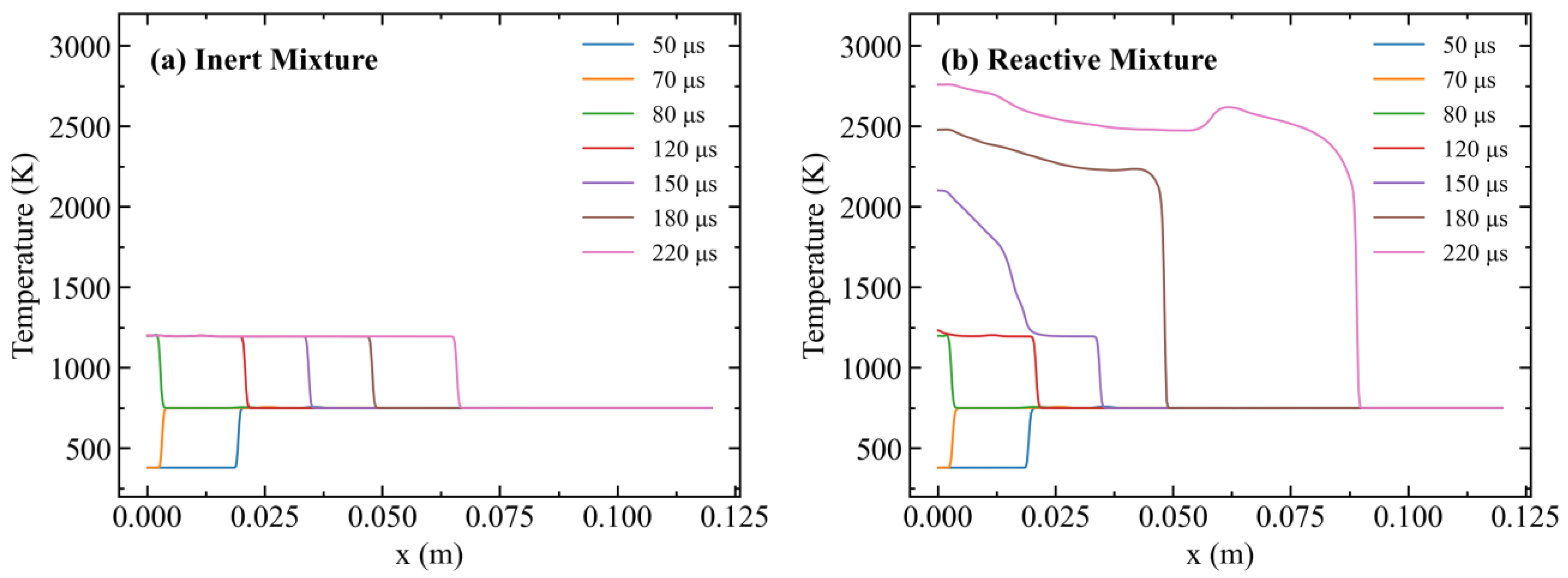
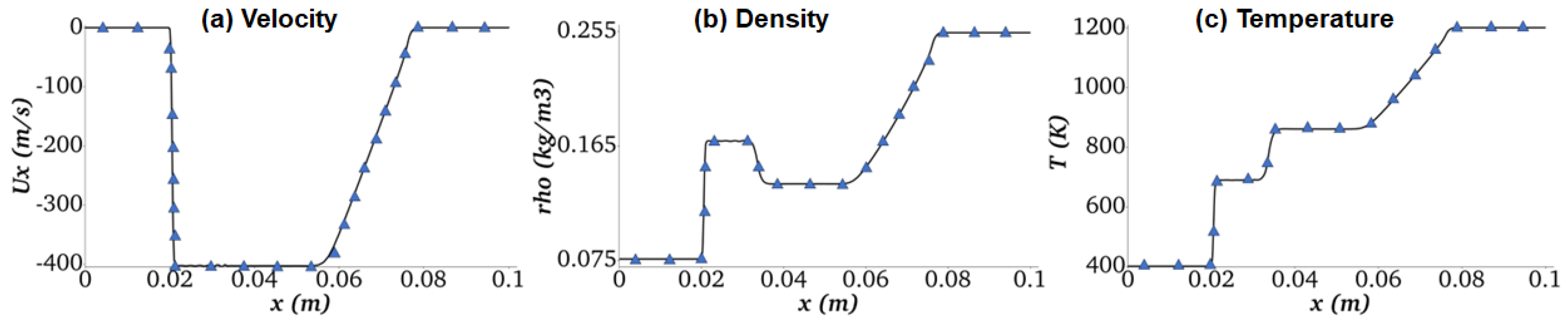
3.1.1. Shock Tube Problem

A shock tube is a well-known benchmark problem (also known as the Sod shock tube problem [55]) for the validation of compressible codes. It is an attractive test case for model validation due to the simple one-dimensional geometry of the computational area and the possibility to simulate a wide range of flow physics, including shock and rarefaction waves, contact discontinuities, and complex wave interactions. The available analytical and computational solutions in the literature allow for the assessment of the code’s accuracy and reliability. The shock tube problems for two cases have been solved: (1) a shock tube with an inert multicomponent gas mixture, and (2) a shock tube with a chemically reactive multicomponent gas mixture. In these validations, the initial discontinuity of the gas in the shock tube is decayed into different gas configurations such as shock waves, contact discontinuities, and rarefaction waves spreading in different directions (See Figure 1).

• Inert Multicomponent Shock Tube

The first validation case is a multicomponent inert shock tube simulation without the chemical source term in order to avoid shock-induced autoignition of the gas mixture. A homogeneous premixed gas mixture of 20%H₂/10%O₂/70%Ar (in mole%) is used in the simulation to verify the numerical accuracy of the model implementations for thermal and mass transport of a multicomponent mixture. The shock tube is 0.10 m in length, and it is discretized with 400 uniform elements. The time step is equal to $∆t={10}^{-7}s$. In the middle of the tube is a fixed diaphragm that separates the gas between the left side ($T_l=400K$ and $P_l=8000Pa$) and the right side ($T_r=1200K$ and $P_r=\mathrm{80,000}Pa$). At time $t=0,$ the diaphragm is eliminated, and the shock wave starts to propagate from right to left and the expansion wave moves in the opposite direction. The initial configuration of the gas mixture generates the propagation of shock and discontinuous waves to the left (low-pressure) and a rarefaction (expansion) wave to the right side (high-pressure) of the tube. Figure 2 shows the current simulation results (solid line) compared with the simulation results of Huang et al. [56]. The modeling results have good agreement. It is noteworthy that the compressibleCentralReactingFoam solver’s accuracy is 2nd order for both time and spatial convective terms.

• Reactive Multicomponent Shock Tube

A reactive multicomponent gas mixture in the shock tube is also modeled using the conditions of Martínez-Ferrer et al. [34] for comparison. The molar composition of the gas mixture is 20% H₂/10% O₂/70% Ar. The length of the tube is equal to $L=0.12m$, with the initial conditions corresponding to the left and right sides as follows: $\left({\rho }_l,u_l,p_l\right)=\left(0.072,0,7173\right)$ and $\left({\rho }_r,u_r,p_r\right)=\left(0.18075,-487.34,\mathrm{35,594}\right)$, where $\rho ,u,\mathrm{a}\mathrm{n}\mathrm{d}p$ are measured in ($kg/m^3$), ($m/s$), and ($Pa$), respectively. The length of the tube is discretized by 400 uniform elements with 0.01 $\mu s$ timestep. The simulation used the reaction mechanism of Conaire et al. [57] for hydrogen, which consists of nine (9) chemical species (H₂, O₂, H, O, OH, HO₂, H₂O₂, H₂O, $Ar$), and 18 elementary reactions. A wall boundary condition is implemented on the left side of the tube, and on the right side, a non-reflected boundary condition is implemented. The initial configuration of non-stable discontinuity is decayed into a shock propagated to the tube’s left side. The solutions of spreading discontinuities in the shock tube for velocity, mass fraction of $H$, and temperature: $U_x$, $Y_H$, and $T$ are shown in Figure 3 for 230 $\mu s$ simulation time. Comparisons of the current solution (solid lines) in Figure 3 with computational data of Martínez-Ferrer et al. [34] (symbols) show good agreement. The visible discrepancies are seen in the vicinities of local maximums around x = 0.06 m at 230 $\mu s$ are explained that Martínez-Ferrer et al. [34] sed a seventh-order accurate Weighted Essentially Non-Oscillatory (WENO) scheme to discretize the non-linear advective terms.

The decay process of the initial multicomponent gas mixture and how the shock wave propagates in the tube were investigated in detail by comparing the profiles of inert and reactive mixtures of H₂/O₂/Ar. Figure 4 shows the simulation results for the temperature profiles of inert and reactive mixtures at various simulation times.

The shock starts to propagate from its initial position in the middle of the tube from right to left toward the wall (i.e., x = 0) with a velocity $v_{rl}$ = 8100 m/s and reaches the wall at around 75 $\mu s$. After reflection from the wall, the shock moves in the opposite direction, from left to right. The reflected shock moves with a velocity of 4500 m/s that is almost half of $v_{rl}$ as the gas flows right to left with a velocity of 490 m/s. Due to the interaction of the shock with the wall, the temperature of the reflected shock is increased from 750 K to 1200 K for both inert and reactive cases. As seen in Figure 4b, the shock-induced autoignition starts to occur (i.e., a slight increase in temperature at x = 0) at 120 $\mu s$ for the reactive case, as the simulation time is longer than the chemical induction time to generate combustion radicals. Due to the combustion heat release, the gas temperature increases to 2100 K as the simulation time approaches 150 $\mu s$. The gas temperature approaches an equilibrium state as the simulation time increases to 220 $\mu s$.

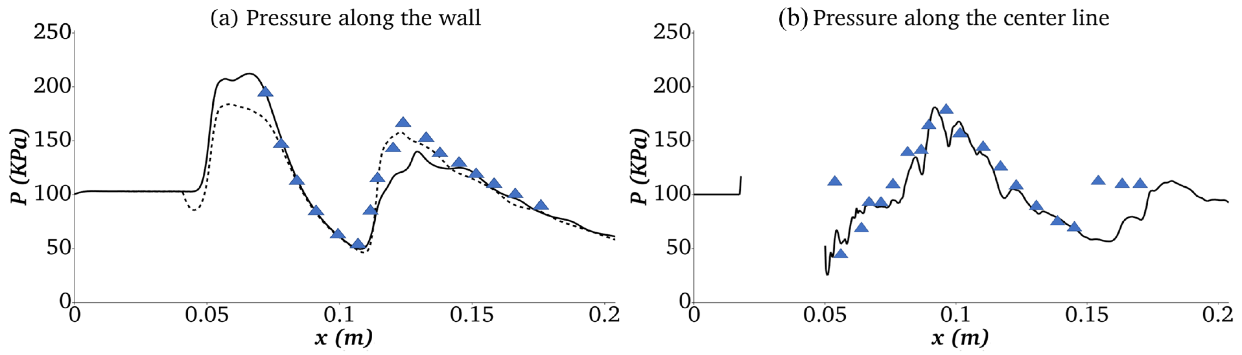
3.1.2. Simulation of Ladenburg Jet Problem

Simulation of a well-known experiment of an underexpanded jet by Ladenburg et al. [58] is conducted to verify code accuracy for the shock formation of supersonic jets. A two-dimensional axisymmetric simulation of the problem using rhoCentralFoam was reported previously [41,59]. In the current work, a 3D simulation of the Ladenburg experiment is performed with the compressibleCentralReactingFoam solver. As the maximum temperature of the experiment is no more than 300 K, the chemical reactions will be in a frozen state, and hence, the gas mixture is considered be inert. The computational 3D mesh (see Figure 5) has a 5 mm inlet radius and 10 mm free surface radius, and is 30 mm in length. The following inlet conditions for pressure, axial velocity and temperature are used to ensure a sonic condition with Mach number of one ($M=1$) at the inlet surface: $2.72·{10}^{5}Pa$, $316.6m/s$ and $247.1K$. The conditions at the free stream surface are $1.01·{10}^{5}Pa$, $0m/s$ and $297K$. Non-reflected boundary conditions are used at the outlet. The simulations are performed using a mesh with total hexahedral elements equal to 1.72 million. A sketch showing wave structures and the simulation flow of Mach number contours is shown in Figure 6a. The pressure at the inlet of the computational region is set by the pressure of the reservoir, which is greater than the ambient pressure; thus, the flow is defined as underexpanded. When air accelerates from high inlet pressure to the atmosphere, the gas flow declines due to its expansion and acceleration. The gas jet expands to the atmospheric pressure through an expansion fan (Figure 6a). This is shown in Figure 6b, in the free jet boundary above which the gas flow is at rest (i.e., $M=0$). In Figure 6a, numbers 1–5 in the circles indicate different gas structures, such as expansion and shock waves. The expansion waves (denoted by 1) are reflected from the free boundary as compression waves. The accumulated compression waves at a point then form an oblique shock wave, shown by the solid line (denoted by 2). The formed oblique shock waves are again reflected off the center line of the flow. This reflection causes the formation of a Mach reflection before the intersection point with the centerline, producing a triple shock point where the compression waves, oblique shock, and centerline coincide. The incoming oblique shock wave (denoted by 2) is the first Mach reflection. The second shock (denoted by 3) is a Mach reflection perpendicular to the centerline, termed a normal (Mach disk) shock. The third Mach reflection (denoted by 4) is another oblique shock wave that is reflected off the constant pressure-free air-jet boundary as an expansion fan (denoted by 5). The escalation of the pressure and temperature occurs as the flow passes through the normal shock or Mach disk. So, the Mach disk is the high-pressure region in an underexpanded air jet that is formed through shock waves and expansion waves created by the vast difference between the inlet pressure and the ambient pressure.

Figure 7 shows a comparison of the current simulation with experimental data of Ladenburg et al. [58] for density iso-lines. The simulation results have good agreement with the experimental data, especially the location and height of the Mach disk. The experimental results show that a weak shock is produced due to the expansion of air from the nozzle orifice (close to density $3.8 kg/m^3$) and then extends toward the nozzle axis. Thus, it creates a Mach disk feature and a triple point (i.e., the intersection of Mach disk, barrel shock and reflected shock). The experimental data in Figure 7 (i.e., lower panel) show that the position of the triple point is at 1.7 mm radial distance and 13.3 mm axial distance. The computed radial and axial distance of the triple point are 1.65 mm and 13.5 mm, respectively. Thus, the computational results yield less than 3% error compared to the experimental data. In summary, the computational results are in good agreement with the experimental data as well as the physics of the shock formation, expansion wave behavior, and their interactions with the jet boundary and slip lines.

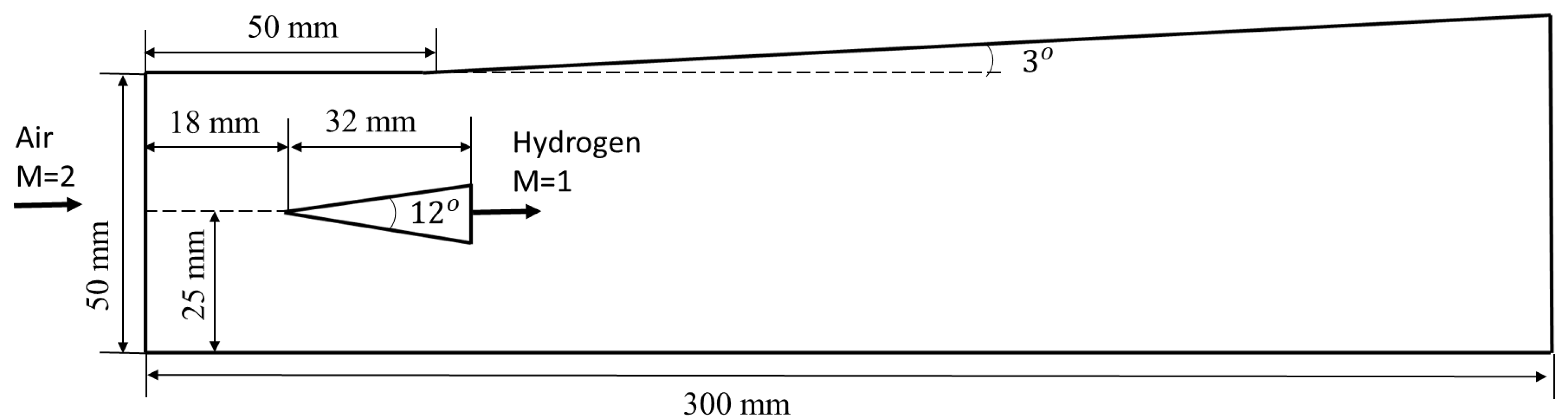
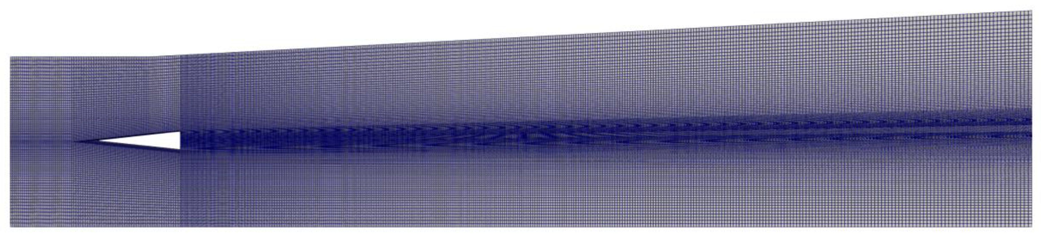
3.1.3. Simulation of DLR Scramjet Combustor

The combustion experiment of Waidmann et al. [60] was selected to validate the compressibleCentralReactingFoam solver to model the turbulence combustion interactions in a scramjet combustor. The experimental data were obtained for hydrogen combustion using the Scramjet test facility at the German Aerospace Center (DLR), with the incoming air flow at Mach number two ($M=2$). The experimental system has been modeled using 2D and 3D computational studies by Oevermann [61] and Haung et al. [35], respectively. Oevermann [61] used RANS (i.e., k-ε turbulence model) with a laminar flamelet, whereas Huang et al. [35] used LES with a PaSR sub-grid scale combustion model to simulate the scramjet. Both computational studies produced reasonable agreement with the experimental data. In the current work, a 2D LES simulation is conducted with a PaSR sub-grid scale combustion model to validate the compressibleCentralReactingFoam solver. Although the two-dimensional assumption may introduce some uncertainty when directly comparing it to the experiment, the 2D computational study will help to verify the accuracy of the model implementation in compressibleCentralReactingFoam qualitatively.

Figure 8 shows the geometry of the DLR test rig. The combustor has a height of $50 \mathrm{mm}$ and width of $45 \mathrm{mm}$ at air inflow. The divergence angle of the upper wall is $3^0$ to compensate for the expansion of the boundary layer. The following boundary conditions for air are established to ensure the Mach number $M_{air}=2$: $u_{air}=730 m/s$, $T_{air}=340 K$, $p_{air}={10}^5 Pa$ with the mass rate of airflow ${\dot{m}}_{air}=1.0kg/s$. The injector of fuel ($H_2$) is a slot in the center of the wedge-shaped strut with a height $∆y_{H2}=0.26 mm$ that gives the surface area of injection $∆s_{H2}=11.7 m{m}^2$. The following boundary conditions are used to establish fuel injector Mach number $M_{H2}=1$: $u_{H2}=1200 m/s$, $T_{H2}=250 K$, $p_{H2}={10}^5 Pa$ with the hydrogen mass flow ${\dot{m}}_{H2}\approx 1.26 g/s$. The no-slip boundary conditions are implemented on the solid walls. The computational region is discretized on 100,000 hexahedrons (See Figure 9). A detailed kinetic mechanism for hydrogen combustion with 9 species and 18 elementary reactions [62] is used. The reaction rates are expressed in Arrhenius form as described in Equations (24)–(28) using the preexponent constant $A_{fj}$, the temperature exponent ${\beta }_j$, and the activation temperature $T_{aj}$.

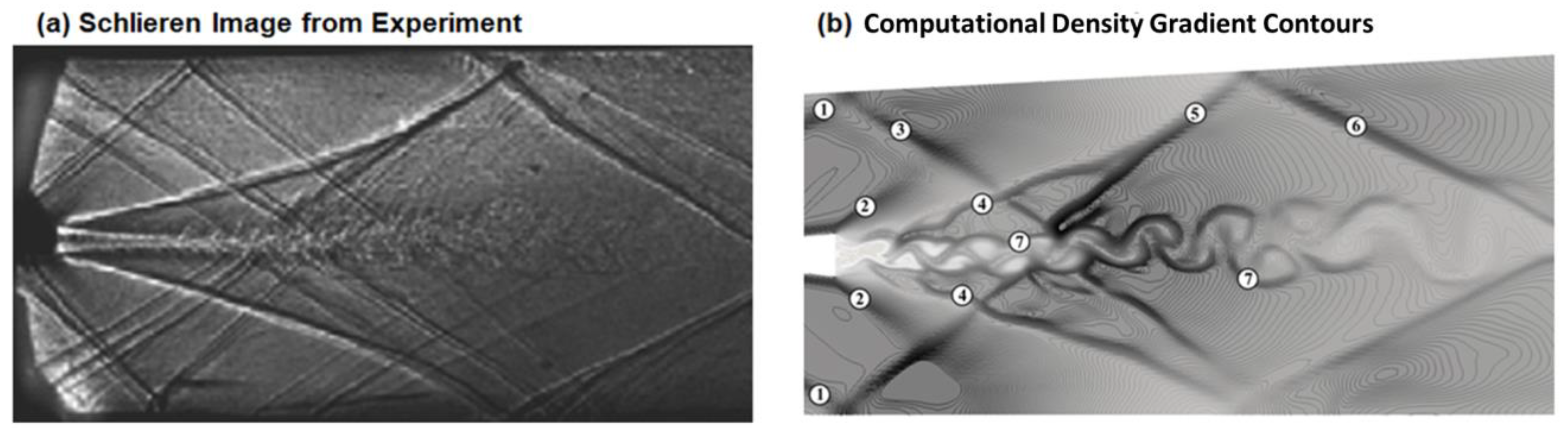
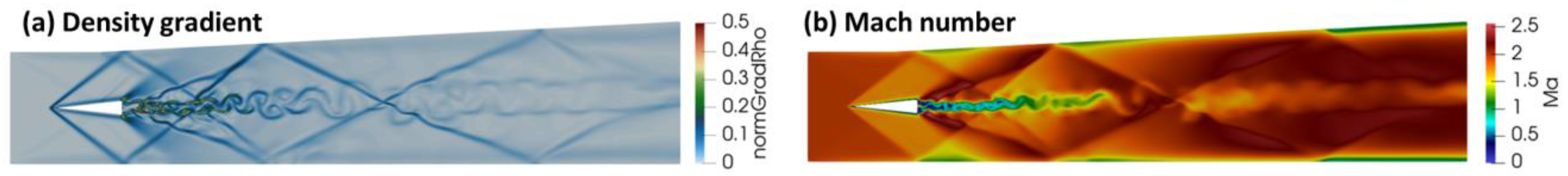
• Simulation of Cold Flow DLR Combustor

Initially, a cold flow case is simulated. Figure 10 shows a Schlieren photograph of the channel flow and computational data of density gradient contours corresponding to the experiment. Comparisons of these two pictures show that the current compressible solver is able to accurately capture the aerodynamic features such as shock waves, expansion waves, interaction, and reflection of these structures from the walls and jet-shear layer. The computational results shown in Figure 10b also identify various flow characteristics with labels 1 to 7. Label (1) shows the leading shocks formed on the tip of the edge (see Figure 10). Label (2) refers to the expansion waves due to the supersonic flow past the corners of the edge. Label (3) is the reflected shock of (1) from the upper wall, whereas label (4) refers to the shocks formed due to collision of gas flow passing through the corner of the edge. Label (5) is an oblique shock formed from merging of the reflected shock and shocks in (4). Lebel (6) is an oblique shock reflected from the upper wall, whereas label (7) is the jet-shear layer formed from the Kelvin–Helmholtz instability. The oblique shocks that are reflected from the upper and lower walls interact with the jet-shear layer, to be reflected again without penetration, as shown Figure 10b.

Figure 11a shows the normalized contours of density gradient $|\mathsf{\nabla }\rho /{\rho }_{max}|$. Figure 11b shows the Mach numbers of the cold flow. Shocks are generated from the tip of the wedge and are further reflected from the lower and upper walls of the combustor. Also, the expansion wave on the upper wall at the starting divergence is seen. Gas flow passing the corners of the wedge is subjected to expansion by forming two expansion waves. The jet vortex structure arises from the Kelvin–Helmholtz instability of the jet-shear layer [14]. It is noteworthy that the simulation with the $k-\epsilon$ turbulence model did not generate shear-layer instabilities as reported by Oevermann [61]. This finding confirms that $RANS$ models are limited when predicting such phenomena and $LES$ models are more appropriate in scramjet combustor simulations.

Figure 12 compares the cold flow simulation results for pressure distributions with the experimental measurements of Waidmann et al. [60]. Figure 12a shows the distribution of pressure on the lower (solid line) and upper (dashed line) walls along with experimental data obtained on the lower wall (symbols). Figure 12b compares the pressure along the center line with the experimental data. The model predictions are able to capture the pressure profiles observed experimentally.

• Simulation of Reacting Flow DLR Combustor

Simulations were performed for reactive flow with a detailed hydrogen kinetic mechanism for experimental conditions of Waidmann et al. [60]. Combustion was initiated with the help of an igniter during the test, as no autoignition was observed experimentally. Our initial simulation also showed that combustion did not occur without an external ignition source. Hence, ignition zones at the two corners of the strut with temperature $T_{ign}=1500 K$ were implemented. Figure 13 compares a Schlieren image of the reactive flow with the computational data for the density contours obtained in the current work for the experimental condition of Waidmann et al. [60]. The comparison shows similar gas dynamic features such as shock waves, expansion waves, interaction, and reflection of the flow structures from the walls and jet-shear layer. Significant gas dynamic differences can be seen between cold flow (Figure 10) and hot flow (Figure 13). For example, expansion waves (i.e., labeled 2 in Figure 10) at the corners of the wedge in cold flow are replaced with the shocks generated due to the combustion in Figure 13. It should be noted that a considerable subsonic region developed behind the hydrogen injection for the reactive flow case.

Figure 14 shows the mean axial velocity along the center line of the DLR combustor. The numerical solution had good agreement with the experimental data.

3.2. Influence of Turbulence Models on Scramjet Combustion

A discussion on the influence of different turbulence models on supersonic combustion is presented in this section. Scramjet simulations for the DLR Scramjet experiment [60] were performed with the following turbulence models described in Section 2.2: SMG, LDkEqn, and WALE. Figure 15 compares the experimental data for temperature at three cross-sections along the combustor with the simulation results obtained with three turbulence models. The numerical results shown in Figure 15 were obtained at $1 ms$ simulation time. The figure also shows the location of the temperature measurements in the DLR Scramjet combustor. The results close to the strut (i.e., x = 62 mm) show that the SMG and WALE models had similar profiles. Further downstream (i.e., x = 216 mm), all three models had similar profiles. Overall, the WALE model had slightly better agreement with the experimental data.

Figure 16 compares the current WALE model simulation results with other DLR Scramjet simulation data reported in the literature [12,30,61,63]. The modeling results of Berglund and Fureby [63] closely followed the experimental profile except at x = 62 mm. Overall, the present model had better agreement with the experimental data at all locations, but it did show relatively higher diffusivity at downstream locations (i.e., x = 108 mm and 216 mm).

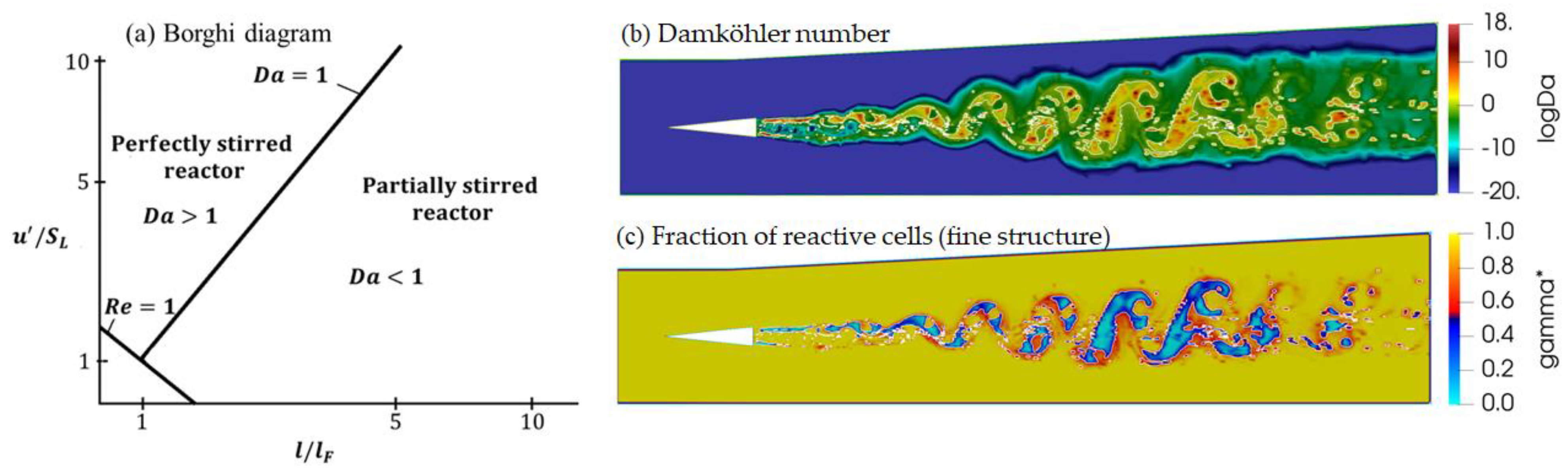
3.3. Analysis of Turbulence–Combustion Interaction in Scramjet Combustor

Based on the analysis of different turbulence models, the WALE model was selected as the most suitable for scramjet simulation. The effect of turbulence–combustion coupling on gas dynamics and flame structure is discussed in this section using the DLR Scramjet simulation results obtained with the WALE model. Figure 17 shows the Mach number (Ma), rate of heat release per unit volume (Qdot), instantaneous temperature (T), and normalized contour lines of density gradient ($|\mathsf{\nabla }\rho /{\rho }_{\mathrm{m}\mathrm{a}\mathrm{x}}|$) obtained from the simulation. The shock structure, shown in Figure 17a,d, is characterized by strong interaction with the shear layers characterized by large density gradients. Behind the strut, a central recirculation bubble is generated with a subsonic region. The formation of the recirculation zone is very important for flame holding and, hence, stabilizing the flame in the scramjet combustor. The rate of heat release contours in Figure 17b show that combustion is intensive within the thin shear layers. The combustion is initiated within the shear layers separated by the recirculation zone close to the edges of the strut. This observation is supported by the temperature data presented in Figure 15a.

The direction of diffusive spreading of fuel and oxidizer helps to analyze turbulence–chemistry interactions. It can be estimated by the interaction between the gradients of fuel ($\mathsf{\nabla }{Y}_F$) and oxygen ($\mathsf{\nabla }{Y}_O$) mass fractions. Takeno and co-workers [64] suggested the use of a flame index (known as the Takeno Flame Index—TFI) based on scalar productions of the gradients of the fuel and oxidizer mass fraction, which help to distinguish between the premixed and non-premixed zones [64]. The TFI is defined as $G_{FO}=(\mathsf{\nabla }{Y}_F·\mathsf{\nabla }{Y}_O)/\left(\left|\mathsf{\nabla }{Y}_F\right|\right|\mathsf{\nabla }{Y}_O\left|\right)$. Positive and negative values of TFI indicate non-premixed or premixed modes, respectively [64]. Figure 18 shows the TFI calculated for the DLR Scramjet conditions. Pockets of non-premixed zones shown in red are surrounded by large premixed zone shown in dark blue.

Figure 19 shows the species mass fraction contours for $OH$, $H$, $H{O}_2$ and $H_{2}O$. It is observed [9] that the OH field is far from uniform in the mixture due to turbulence, which would have been expected from fast chemistry arguments. High OH regions are found where the mixture fraction iso-surfaces are highly convoluted, and low values are in the areas where the mixture fraction iso-surfaces are stretched and not wrinkled. The mass fraction of OH is relatively small at the beginning, while it is most prominent in the downstream regions, especially in the transition zone. The OH radical represents the existence of a flame front that correlates with the heat release rate. The field of H₂O correlates with the field of instantaneous temperature, while the field of HO₂ correlates with OH and Qdot on the shear layer.

Figure 20 shows mixture fraction ($Z$) and scalar dissipation rate ($\chi )$. The mixture fraction measures the local fuel/oxidizer ratio and is calculated as $Z=(\phi ·Y_F/Y_{F0}-Y_O/Y_{O0}+1)/(\phi +1)$, where $\phi$ is the equivalence ratio. The scalar dissipation rate is calculated as $\chi =2D(\mathsf{\nabla }Z·\mathsf{\nabla }Z)$, where $D$ is the mixture diffusion coefficient. The scalar dissipation rate is essentially the rate of mixing between fuel and oxidizer [9] and represents the local mixing rate at the molecular level [65]. The scalar dissipation rate is critical for modeling the effect of turbulence on reaction rates, as it has significant influence on non-premixed combustion. It often provides the connection between the molecular mixing and the combustion. In turbulent flows, the scalar dissipation is seen as a scalar energy dissipation. Its role is to destroy (dissipate) scalar variance (scalar energy), analogous to the dissipation of the turbulence. Unlike the kinetic energy dissipation, most of the scalar dissipation occurs at the finest scales. The scalar dissipation has higher values near the strut and decreases further downstream as shown in Figure 20b.

A time-scale analysis based on the estimation of the local Damköhler Number (Da) was also performed to examine the reactive zones in more detail. The Da number was quantified as the ratio between the turbulent mixing time scale ${\tau }^{*}$ (Equation (32)) and the chemical time scale ${\tau }_c$: $Da={\tau }^{*}/{\tau }_c$ [66,67]. The Borghi diagram [68] shown in Figure 21a helps to recognize different regimes of turbulent combustion, where $l$ is the characteristic size of flow geometry, $l_F$ is the laminar flame thickness, $u^{\prime }$ is characteristic velocity in the order of turbulence intensity, and $S_L$ is the laminar flame speed. Figure 21b,c show the Damköhler number (Da) on a logarithmic scale and the fraction of fine structure (${\gamma }^{*}$), respectively. The bright white lines indicate the locations where $Da=1$. The Damköhler number is relatively high ($Da>1$) in the core of the jet flow. This indicates that the time scale of chemical reaction is smaller than the turbulent mixing time scale, which means a combustion regime with fast chemistry. Thus, the fraction of reactive cells (${\gamma }^{*}$) (see Equation (31) for details) is mostly small in this zone. In contrast, in the shear layer, where the rates of heat release (see Figure 17b) and scalar dissipation (see Figure 20b) have the highest values, the flame is controlled by finite rate chemistry with $Da<1$ and $0<{\gamma }^{*}<1.$ This combustion regime is characterized as a partially stirred reactor. In the core flow, small pockets where $Da<1$ are also seen, indicating the combustion zone is in the “island formation” regime (see Figure 14.2 in Warnatz, et al. [66]).

4. Conclusions

A computational validation of a new compressibleCentralReactingFoam code for modeling combustion in supersonic flows was presented. The validation cases included various complexities of high-speed flows with shocks, wave expansion, and turbulence–combustion interactions. Comparisons of the simulation results with data in the literature demonstrated the numerical fidelity of the solver for reactive multicomponent gas mixtures at supersonic conditions. In addition, a detailed analysis of gas dynamics and turbulence–combustion interaction under supersonic conditions was presented to gain a deeper understanding of the complex physical-chemical phenomena involved. A comparative analysis of the influence of three turbulent subgrid models on scramjet combustion was presented. The comparison of simulation results with the experimental data showed that the WALE subgrid scale is most suitable for scramjet modeling. The DLR scramjet simulation results showed that the flame was mainly stabilized in the combustor due to the formation of a subsonic bubble behind the strut. The supersonic flame structure was investigated through a comprehensive analysis of chemical species formation, scalar dissipation rate, flame index, heat release rate, fine structure, and Damköhler number. A time-scale analysis based on the local Damköhler number revealed different regimes of turbulence combustion in the scramjet. In the core of the jet flow, the Da number was relatively high ($Da>1$), indicating that the chemical time scale was smaller than the turbulent mixing time scale. This means that the combustion regime was dominated by fast chemistry. The results also showed that the heat release rate and the scalar dissipation rate had the highest values in the shear layer, and the flame was stabilized due to finite rate chemistry with $Da<1$ and $0<{\gamma }^{*}<1$. Thus, the new solver presented in this paper can be used for high-speed simulations of multicomponent reactive gas mixtures in supersonic combustors.

References

1. Urzay, J. Supersonic Combustion in Air-Breathing Propulsion Systems for Hypersonic Flight. Annu. Rev. Fluid Mech. 2018, 50, 593–627. [Google Scholar] [CrossRef]
2. Fureby, C. Large eddy simulation modelling of combustion for propulsion applications. Philos. Trans. R. Soc. A Math. Phys. Eng. Sci. 2009, 367, 2957–2969. [Google Scholar] [CrossRef]
3. Abdulrahman, G.A.Q.; Qasem, N.A.A.; Imteyaz, B.; Abdallah, A.M.; Habib, M.A. A review of aircraft subsonic and supersonic combustors. Aerosp. Sci. Technol. 2023, 132, 108067. [Google Scholar] [CrossRef]
4. O’Byrne, S.; Doolan, M.; Olsen, S.R.; Houwing, A.F.P. Measurement and imaging of supersonic combustion in a model scramjet engine. Shock Waves 1999, 9, 221–226. [Google Scholar] [CrossRef]
5. Menon, S.; Sankaran, V.; Stone, C. Subgrid Combustion Modeling for the Next Generation National Combustion Code. CCL-02–003, April 2003. Available online: https://ntrs.nasa.gov/citations/20030038812 (accessed on 30 November 2023).
6. Menon, S.; Fureby, C. Computational Combustion. In Encyclopedia of Aerospace Engineering; John Wiley & Sons, Ltd.: Hoboken, NJ, USA, 2010; ISBN 978-0-470-68665-2. [Google Scholar]
7. Sagaut, P. Large Eddy Simulation for Incompressible Flows; Scientific Computation; Springer: Berlin/Heidelberg, Germany, 2006; ISBN 978-3-540-26344-9. [Google Scholar]
8. Echekki, T.; Mastorakos, E. (Eds.) Turbulent Combustion Modeling: Advances, New Trends and Perspectives; Fluid Mechanics and Its Applications; Springer: Dordrecht, The Netherlands, 2011; Volume 95. [Google Scholar] [CrossRef]
9. Hawkes, E.R.; Sankaran, R.; Sutherland, J.C.; Chen, J.H. Direct numerical simulation of turbulent combustion: Fundamental insights towards predictive models. J. Phys. Conf. Ser. 2005, 16, 65. [Google Scholar] [CrossRef]
10. Gutiérrez, L.F.; Universidad Nacional de Córdoba-IDIT(CONICET); Tamagno, J.; Univeridad Nacional de Córdoba; Elaskar, S.A. Univeridad Nacional de Córdoba-CONICET RANS Simulation of Turbulent Diffusive Combustion using Open Foam. JAFM 2016, 9, 669–682. [Google Scholar] [CrossRef]
11. Ingenito, A.; Bruno, C. Physics and Regimes of Supersonic Combustion. AIAA J. 2010, 48, 515–525. [Google Scholar] [CrossRef]
12. Génin, F.; Menon, S. Simulation of Turbulent Mixing Behind a Strut Injector in Supersonic Flow. AIAA J. 2010, 48, 526–539. [Google Scholar] [CrossRef]
13. Fureby, C.; Nordin-Bates, K.; Petterson, K.; Bresson, A.; Sabelnikov, V. A computational study of supersonic combustion in strut injector and hypermixer flow fields. Proc. Combust. Inst. 2015, 35, 2127–2135. [Google Scholar] [CrossRef]
14. Fureby, C.; Sahut, G.; Ercole, A.; Nilsson, T. Large Eddy Simulation of Combustion for High-Speed Airbreathing Engines. Aerospace 2022, 9, 785. [Google Scholar] [CrossRef]
15. Gokulakrishnan, P.; Foli, K.; Klassen, M.; Roby, R.; Soteriou, M.; Kiel, B.; Sekar, B. LES-PDF Modeling of Flame Instability and Blow-out in Bluff-Body Stabilized Flames. In Proceedings of the 45th AIAA/ASME/SAE/ASEE Joint Propulsion Conference & Exhibit, Denver, CO, USA, 2–5 August 2009; American Institute of Aeronautics and Astronautics: Reston, VA, USA, 2009. [Google Scholar]
16. Gokulakrishnan, P.; Bikkani, R.; Klassen, M.; Roby, R.; Kiel, B. Influence of Turbulence-Chemistry Interaction in Blow-out Predictions of Bluff-Body Stabilized Flames. In Proceedings of the 47th AIAA Aerospace Sciences Meeting Including the New Horizons Forum and Aerospace Exposition, Orlando, FL, USA, 5–8 January 2009; American Institute of Aeronautics and Astronautics: Reston, VA, USA, 2009. [Google Scholar]
17. Dasgupta, A.; Gonzalez-Juez, E.; Haworth, D.C. Flame simulations with an open-source code. Comput. Phys. Commun. 2019, 237, 219–229. [Google Scholar] [CrossRef]
18. Gonzalez-Juez, E.D.; Dasgupta, A.; Arshad, S.; Oevermann, M.; Lignell, D. Effect of the turbulence modeling in large-eddy simulations of nonpremixed flames undergoing extinction and reignition. In Proceedings of the AIAA SciTech Forum—55th AIAA Aerospace Sciences Meeting, Grapevine, TX, USA, 9–13 January 2017. [Google Scholar]
19. Gonzalez-Juez, E.D.; Kerstein, A.R.; Ranjan, R.; Menon, S. Advances and challenges in modeling high-speed turbulent combustion in propulsion systems. Prog. Energy Combust. Sci. 2017, 60, 26–67. [Google Scholar] [CrossRef]
20. Peters, N. Turbulent Combustion, 1st ed.; Cambridge University Press: Cambridge, UK, 2000; ISBN 978-0-521-66082-2. [Google Scholar]
21. Pope, S.B. Small scales, many species and the manifold challenges of turbulent combustion. Proc. Combust. Inst. 2013, 34, 1–31. [Google Scholar] [CrossRef]
22. Huang, S.; Chen, Q.; Cheng, Y.; Xian, J.; Tai, Z. Supersonic Combustion Modeling and Simulation on General Platforms. Aerospace 2022, 9, 366. [Google Scholar] [CrossRef]
23. Piasecka, M.; Piasecki, A.; Dadas, N. Experimental Study and CFD Modeling of Fluid Flow and Heat Transfer Characteristics in a Mini-Channel Heat Sink Using Simcenter STAR-CCM+ Software. Energies 2022, 15, 536. [Google Scholar] [CrossRef]
24. Edwards, J.R.; Fulton, J.A. Development of a RANS and LES/RANS Flow Solver for High-Speed Engine Flowpath Simulations. In Proceedings of the 20th AIAA International Space Planes and Hypersonic Systems and Technologies Conference, Glasgow, UK, 6–9 July 2015; American Institute of Aeronautics and Astronautics: Reston, VA, USA, 2015. [Google Scholar]
25. Nelson, C. An Overview of the NPARC Alliance’s Wind-US Flow Solver. In Proceedings of the 48th AIAA Aerospace Sciences Meeting Including the New Horizons Forum and Aerospace Exposition, Orlando, Fl, USA, 4–7 January 2010; American Institute of Aeronautics and Astronautics: Reston, VA, USA, 2010. [Google Scholar]
26. Steelant, J.; Mack, A.; Hannemann, K.; Gardner, A. Comparison of Supersonic Combustion Tests with Shock Tunnels, Flight and CFD. In Proceedings of the 42nd AIAA/ASME/SAE/ASEE Joint Propulsion Conference & Exhibit, Sacramento, CA, USA, 9–12 July 2006; American Institute of Aeronautics and Astronautics: Reston, VA, USA, 2006. [Google Scholar]
27. Drummond, J.P.; Danehy, P.M.; Gaffney, R.L.; Tedder, S.A.; Cutler, A.D.; Bivolaru, D. Supersonic Combustion Research at NASA. In Proceedings of the 2007 Fall Technical Meeting—Eastern States Section of the Combustion Institute, Charlottesville, VA, USA, 21–24 October 2007; Available online: https://ntrs.nasa.gov/citations/20080013391 (accessed on 30 November 2023).
28. Palacios, F.; Economon, T.; Aranake, A.; Copeland, S.; Lonkar, A.K.; Lukaczyk, T.; Manosalvas, D.E.; Naik, K.R.; Padr, A.S.; Tracey, B.D.; et al. Stanford University Unstructured (SU 2): Open-source Analysis and Design Technology for Turbulent Flows. 2014. Available online: https://www.semanticscholar.org/paper/Stanford-University-Unstructured-(SU-2-)%3A-Analysis-Palacios-Economon/3b6dd8951b4d1e30fca73c8e737585ec920d81b0.
29. Weller, H.G.; Tabor, G.; Jasak, H.; Fureby, C. A tensorial approach to computational continuum mechanics using object-oriented techniques. Comput. Phys. 1998, 12, 620–631. [Google Scholar] [CrossRef]
30. Zhang, H.; Zhao, M.; Huang, Z. Large eddy simulation of turbulent supersonic hydrogen flames with OpenFOAM. Fuel 2020, 282, 118812. [Google Scholar] [CrossRef]
31. Chapuis, M.; Fedina, E.; Fureby, C.; Hannemann, K.; Karl, S.; Martinez Schramm, J. A computational study of the HyShot II combustor performance. Proc. Combust. Inst. 2013, 34, 2101–2109. [Google Scholar] [CrossRef]
32. Droeske, N.; Makowka, K.; Nizenkov, P.; Vellaramkalayil, J.J.; Sattelmayer, T.; von Wolfersdorf, J. Validation of a Novel OpenFOAM Solver using a Supersonic, Non-reacting Channel Flow. In Proceedings of the 19th AIAA International Space Planes and Hypersonic Systems and Technologies Conference, Atlanta, GA, USA, 16–20 June 2014; AIAA Aviation Forum. American Institute of Aeronautics and Astronautics: Reston, VA, USA, 2014. [Google Scholar]
33. Makowka, K.; Droeske, N.; Vellaramkalayil, J.J.; Sattelmayer, T.; von Wolfersdorf, J. Unsteady RANS Investigation of a Hydrogen-Fueled Staged Supersonic Combustor with Lobed Injectors. In Proceedings of the 19th AIAA International Space Planes and Hypersonic Systems and Technologies Conference, Atlanta, GA, USA, 16–20 June 2014; AIAA Aviation Forum. American Institute of Aeronautics and Astronautics: Reston, VA, USA, 2014. [Google Scholar]
34. Martínez-Ferrer, P.J.; Buttay, R.; Lehnasch, G.; Mura, A. A detailed verification procedure for compressible reactive multicomponent Navier–Stokes solvers. Comput. Fluids 2014, 89, 88–110. [Google Scholar] [CrossRef]
35. Huang, Z.; He, G.; Qin, F.; Wei, X. Large eddy simulation of flame structure and combustion mode in a hydrogen fueled supersonic combustor. Int. J. Hydrogen Energy 2015, 40, 9815–9824. [Google Scholar] [CrossRef]
36. Arisman, C.J.; Johansen, C.T. Nitric Oxide Chemistry Effects in Hypersonic Boundary Layers. AIAA J. 2015, 53, 3652–3660. [Google Scholar] [CrossRef]
37. Zhou, D.; Zou, S.; Yang, S. An OpenFOAM-based fully compressible reacting flow solver with detailed transport and chemistry for high-speed combustion simulations. In Proceedings of the AIAA SciTech 2020 Forum, Orlando, FL, USA, 6–10 January 2020; American Institute of Aeronautics and Astronautics: Reston, VA, USA, 2020. [Google Scholar]
38. Hoste, J.-J.O.; Casseau, V.; Fossati, M.; Taylor, I.J.; Gollan, R. Numerical Modeling and Simulation of Supersonic Flows in Propulsion Systems by Open-Source Solvers. In Proceedings of the 21st AIAA International Space Planes and Hypersonics Technologies Conference, Xiamen, China, 6–9 March 2017; American Institute of Aeronautics and Astronautics: Reston, VA, USA, 2017. [Google Scholar]
39. Kurganov, A.; Tadmor, E. New High-Resolution Central Schemes for Nonlinear Conservation Laws and Convection–Diffusion Equations. J. Comput. Phys. 2000, 160, 241–282. [Google Scholar] [CrossRef]
40. Kurganov, A.; Noelle, S.; Petrova, G. Semidiscrete Central-Upwind Schemes for Hyperbolic Conservation Laws and Hamilton--Jacobi Equations. SIAM J. Sci. Comput. 2001, 23, 707–740. [Google Scholar] [CrossRef]
41. Greenshields, C.J.; Weller, H.G.; Gasparini, L.; Reese, J.M. Implementation of semi-discrete, non-staggered central schemes in a colocated, polyhedral, finite volume framework, for high-speed viscous flows. Int. J. Numer. Methods Fluids 2010, 63, 1–21. [Google Scholar] [CrossRef]
42. OpenFOAM v2306. Available online: https://www.openfoam.com/news/main-news/openfoam-v2306 (accessed on 30 November 2023).
43. Smagorinsky, J. General Circulation Experiments with the Primitive Equations. Mon. Weather Rev. 1963, 91, 99. [Google Scholar] [CrossRef]
44. Erlebacher, G.; Hussaini, M.Y.; Speziale, C.G.; Zang, T.A. Toward the large-eddy simulation of compressible turbulent flows. J. Fluid Mech. 1992, 238, 155–185. [Google Scholar] [CrossRef]
45. Kim, W.-W.; Menon, S. A new dynamic one-equation subgrid-scale model for large eddy simulations. In Proceedings of the 33rd Aerospace Sciences Meeting and Exhibit, Reno, NV, USA, 9–12 January 1995; American Institute of Aeronautics and Astronautics: Reston, VA, USA, 1995. [Google Scholar]
46. Huang, S.; Li, Q.S. A new dynamic one-equation subgrid-scale model for large eddy simulations. Int. J. Numer. Methods Eng. 2010, 81, 835–865. [Google Scholar] [CrossRef]
47. Nicoud, F.; Ducros, F. Subgrid-Scale Stress Modelling Based on the Square of the Velocity Gradient Tensor. Flow Turbul. Combust. 1999, 62, 183–200. [Google Scholar] [CrossRef]
48. Berglund, M.; Fedina, E.; Fureby, C.; Tegnér, J.; Sabel’nikov, V. Finite Rate Chemistry Large-Eddy Simulation of Self-Ignition in Supersonic Combustion Ramjet. AIAA J. 2010, 48, 540–550. [Google Scholar] [CrossRef]
49. Mcbride, B.J.; Gordon, S.; Reno, M.A. Coefficients for Calculating Thermodynamic and Transport Properties of Individual Species. NASA-TM-4513, October 1993. Available online: https://ntrs.nasa.gov/citations/19940013151 (accessed on 3 January 2024).
50. Sabelnikov, V.; Fureby, C. Extended LES-PaSR model for simulation of turbulent combustion. Prog. Propuls. Phys. 2013, 4, 539–568. [Google Scholar]
51. Baudoin, E.; Yu, R.; Bai; Nogenmur, K.J.; Bai, X.-S.; Fureby, C. Comparison of LES Models Applied to a Bluff Body Stabilized Flame. In Proceedings of the 47th AIAA Aerospace Sciences Meeting including The New Horizons Forum and Aerospace Exposition, Orlando, FL, USA, 5–8 January 2009; American Institute of Aeronautics and Astronautics: Reston, VA, USA, 2009. [Google Scholar]
52. Magnussen, B. On the structure of turbulence and a generalized eddy dissipation concept for chemical reaction in turbulent flow. In Proceedings of the 19th Aerospace Sciences Meeting, St. Louis, MO, USA, 12–15 January 1981; American Institute of Aeronautics and Astronautics: Reston, VA, USA, 1981. [Google Scholar]
53. Behrens, T. OpenFOAM’s Basic Solvers for Linear Systems of Equations; Chalmers University of Technology: Göteborg, Sweden, 2009. [Google Scholar]
54. Mitchell, A.R.; Griffiths, D.F. The Finite Difference Method in Partial Differential Equations, 1st ed.; Wiley: Chichester, UK; New York, NY, USA, 1980; ISBN 978-0-471-27641-8. [Google Scholar]
55. Sod, G.A. A survey of several finite difference methods for systems of nonlinear hyperbolic conservation laws. J. Comput. Phys. 1978, 27, 1–31. [Google Scholar] [CrossRef]
56. Huang, Z.; Zhao, M.; Xu, Y.; Li, G.; Zhang, H. Eulerian-Lagrangian modelling of detonative combustion in two-phase gas-droplet mixtures with OpenFOAM: Validations and verifications. Fuel 2021, 286, 119402. [Google Scholar] [CrossRef]
57. Ó Conaire, M.; Curran, H.J.; Simmie, J.M.; Pitz, W.J.; Westbrook, C.K. A comprehensive modeling study of hydrogen oxidation. Int. J. Chem. Kinet. 2004, 36, 603–622. [Google Scholar] [CrossRef]
58. Ladenburg, R.; Van Voorhis, C.C.; Winckler, J. Interferometric Studies of Faster than Sound Phenomena. Part II. Analysis of Supersonic Air Jets. Phys. Rev. 1949, 76, 662–677. [Google Scholar] [CrossRef]
59. Talukdar, M. Numerical Simulation of Underexpanded Air Jet Using OpenFOAM. Master’s Thesis, University of Stavanger, Stavanger, Norway, 2015. Available online: https://uis.brage.unit.no/uis-xmlui/handle/11250/302085 (accessed on 30 November 2023).
60. Waidmann, W.; Alff, F.; Böhm, M.; Brummund, U.; Clauss, W.; Oschwald, M. Supersonic Combustion of Hydrogen/Air in a Scramjet Combustion Chamber. Space Technol. 1994, 6, 421–429. Available online: https://www.semanticscholar.org/paper/Supersonic-Combustion-of-Hydrogen-Air-in-a-Scramjet-Waidmann-Alff/a110e9db66cdc1d568a023ab14bada917d2d5113 (accessed on 22 January 2024).
61. Oevermann, M. Numerical investigation of turbulent hydrogen combustion in a SCRAMJET using flamelet modeling. Aerosp. Sci. Technol. 2000, 4, 463–480. [Google Scholar] [CrossRef]
62. Maas, U.; Warnatz, J. Ignition processes in hydrogen oxygen mixtures. Combust. Flame 1988, 74, 53–69. [Google Scholar] [CrossRef]
63. Berglund, M.; Fureby, C. LES of supersonic combustion in a scramjet engine model. Proc. Combust. Inst. 2007, 31, 2497–2504. [Google Scholar] [CrossRef]
64. Yamashita, H.; Shimada, M.; Takeno, T. A numerical study on flame stability at the transition point of jet diffusion flames. Symp. (Int.) Combust. 1996, 26, 27–34. [Google Scholar] [CrossRef]
65. Bilger, R.W. Some Aspects of Scalar Dissipation. Flow Turbul. Combust. 2004, 72, 93–114. [Google Scholar] [CrossRef]
66. Warnatz, J.; Maas, U.; Dibble, R.W. Combustion; Springer: Berlin/Heidelberg, Germany, 2006; ISBN 978-3-540-25992-3. [Google Scholar]
67. Poinsot, T.; Veynante, D. Theoretical and Numerical Combustion, 2nd ed.; R T Edwards Inc.: Philadelphia, PA, USA, 2005; ISBN 978-1-930217-10-2. [Google Scholar]
68. Borghi, R. On the Structure and Morphology of Turbulent Premixed Flames. In Recent Advances in the Aerospace Sciences: In Honor of Luigi Crocco on His Seventy-Fifth Birthday; Casci, C., Bruno, C., Eds.; Springer: Boston, MA, USA, 1985; pp. 117–138. ISBN 978-1-4684-4298-4. [Google Scholar]
Figure 1. Shock tube and spreading shock wave (red), the contact surface (black), and expansion fan (blue).
Dynamics 04 00008 g001
Figure 2. Multicomponent inert shock tube profiles of H2/O2/Ar mixture at 40 μs. Keys: solid line—current simulation; symbols—simulation of Huang et al. [56].
Dynamics 04 00008 g002
Figure 3. Multicomponent reactive shock tube profiles of H2/O2/Ar mixture at 230 μs. Keys: solid line—current simulation; symbols—Martínez-Ferrer et al. [34].
Dynamics 04 00008 g003
Figure 4. Temperature profiles of shocks/detonation waves for (a) inert and (b) reactive mixture at various times.
Dynamics 04 00008 g004
Figure 5. Computational 3D mesh for simulation of underexpanded jet of Ladenburg experiment. Inflow is shown by the yellow surface, the free stream inlet surface is violet, and the free stream surface is red.
Dynamics 04 00008 g005
Figure 6. (a) Schematics of an underexpanded air jet. Keys: 1 expansion waves, 2 oblique shock, 3 normal shock, 4 reflected shock, 5 reflected expansion waves. (b) Contours of Mach numbers at the plane through the center of computational domain (see Figure 5).
Dynamics 04 00008 g006
Figure 7. Density distribution of the supersonic jet measured (reprinted with permission from Ladenburg [58]) (lower panel), compared with current computational results (upper panel). The values of the density contours are provided in kg/m3.
Dynamics 04 00008 g007
Figure 8. Geometry of DLR experiment [60]. The 12° wedge provides a stagnation zone for flame holding.
Dynamics 04 00008 g008
Figure 9. Computational 2D mesh for simulation of turbulence combustion in DLR.
Dynamics 04 00008 g009
Figure 10. (a) Cold flow Schlieren image of the channel with hydrogen injection (reprinted with permission from [60,61]). (b) Computational density gradient contours corresponding to the experimental image in (a). Labels 1 to 7 in (b) refer to various flow structures discussed in the text.
Dynamics 04 00008 g010
Figure 11. (a) Normalized density gradient contour; (b) Mach numbers for cold flow.
Dynamics 04 00008 g011
Figure 12. (a) Pressure distribution along channel walls. Keys: symbols—experimental data for lower wall [60]; lines—current simulation (solid—lower wall; dashed—the upper wall). (b) Pressure distribution along the centerline. Keys; symbols—experimental data [60]; line—current simulation.
Dynamics 04 00008 g012
Figure 13. (a) Schlieren photograph of the channel flow with hydrogen injection (reprinted with permission from [60,61]); (b) computational density gradient contours corresponding to the experimental conditions.
Dynamics 04 00008 g013
Figure 14. Mean axial velocity profile along the middle of the channel at y = 25   m m . Keys: symbols—experimental data [60]; line—current simulation.
Dynamics 04 00008 g014
Figure 15. Contours of mean temperature (upper) and mean temperature at the three cross-sections with different turbulence models (bottom). Keys: symbols—experimental data [60]; lines—simulation. Color keys: black—WALE; red—SMG; blue—LDkEqn.
Dynamics 04 00008 g015
Figure 16. Mean temperature at three cross-sections compared with simulation data in the literature. Keys: symbols—experimental data [60]; lines—simulation. Color keys: black—current simulation with WALE model; red—Berglund and Fureby [63]; green—Genin and Menon [12]; blue—Zhang et al. [30]; purple—Oevermann [61].
Dynamics 04 00008 g016
Figure 17. Instantaneous distribution of: (a) Mach number; (b) normalized heat release rate Q d o t N o r m = Q d o t / 10 10 ; (c) temperature; (d) normalized contour lines of density gradient.
Dynamics 04 00008 g017
Figure 18. Takeno Flame Index (TFI) [59].
Dynamics 04 00008 g018
Figure 19. Instantaneous distribution of species mass fraction. (a) H; (b) OH; (c) HO2; (d) H2O.
Dynamics 04 00008 g019
Figure 20. Instantaneous distribution of: (a) mixture fraction; (b) scalar dissipation rate χ (in the log scale).
Dynamics 04 00008 g020
Figure 21. (a) Borghi diagram showing different turbulent combustion regimes; (b) Damköhler number (Da in logarithmic scale); (c) fraction of reactive cells ( γ * ). The white lines indicate locations where D a = 1 .
Dynamics 04 00008 g021
Disclaimer/Publisher’s Note: The statements, opinions and data contained in all publications are solely those of the individual author(s) and contributor(s) and not of MDPI and/or the editor(s). MDPI and/or the editor(s) disclaim responsibility for any injury to people or property resulting from any ideas, methods, instructions or products referred to in the content.