The Free Euler Rigid Body Revisited

Abstract

We review from a different perspective the approach and solution to the torque-free Euler equations, also called the free asymmetric top equations. We aim to simplify and broaden the study of the asymmetric free rigid body. This is an old but important integrable problem that has two first integrals: the energy and the angular momentum. We reduce this problem by eliminating the time as the independent variable in the three autonomous Euler equations written in cylindrical dimensionless variables, which allows a geometric study of the solution as a function of the cylindrical angle variable $\psi$, by means of continuous deformations dependent on the two independent parameters $\kappa$ and $e_0$. The parameter space is divided into six disjoint regions, whose boundaries are the separatices and degenerated cases. The solutions are given in terms of trigonometric functions of the independent cylindric angle $\psi$.

1. Introduction

The study of the rigid body dates back to the XVIII century, with the pioneering works of Euler (1707–1783), who dedicated a large part of his life to study this problem, trying to explain and predict the motion of ships and their building (a historical review of Euler’s works on the rigid body are in the article by Marquina et al. [1]). Around 1736, Euler published in two large volumes his treatise Mechanica sive motus scientia analytice exposita (Mechanics or the science of motion, expounded analytically), where he proposes that the motion of a rigid body can be studied as two types of combined movements: one of translation around its center of gravity, and another of rotation of the body’s orientation around an axis that passes through its center of gravity. The most simple rotation problem is when there are no torques, the so called Euler free rigid body or simply the Euler top. In 1755, Segner showed that every rigid body has three main axes where the inertial tensor is diagonal. Then, in the series of works that Euler wrote between 1758 and 1765, which culminate in the voluminous compendium Theoria motus corporum rigorumum seu solidorum, Euler used the principal axes system, and found the so-called Euler equations and the Euler angles. He obtained the kinematic relations for the motion of a heavy rigid body and addressed the integrable problem of the free rigid body, reducing it to quadratures. The angular momentum in the inertial frame is a constant of motion, but in the body-fix frame it satisfies the Euler equations.

A geometric construction of the solution to the Euler equations for the free rigid body was given by Luis Poinsot [2] in 1851 using the polhod and herpolhod: the inertia ellipsoid with a fixed center rolls without slipping on a fixed plane perpendicular to the constant angular momentum; the position vector of the contact point is like an instantaneous axis of rotation, and draws polhodes on the ellipsoid of inertia, or herpolhodes on the fixed plane.

The general solution of the motion of a rigid body around a fixed point under no forces was probably first given by Rueb in 1834 [3] in his PhD Thesis, and completed by Jacobi in 1849 [4], who obtained the Euler angles in terms of elliptic functions and theta functions, and their expression in terms of Fourier series. Elliptic integrals had already appeared in the Elastica of Jakob Bernoulli, while Maclaurin, Fragano, Legendre and others used them in connection with the problem of rectifying an arc of an ellipse. Proceeding in analogy with the circular functions, Abel, Jacobi, Gauss and Weierstrass [5] introduced the idea of inverting the elliptic integrals defining the elliptic functions. Carl Gauss noticed that the rigid body position may be uniquely determined by quaternions with unit norm, now known as the Rodrigues–Hamilton parameters [6].

Integrable cases of the rigid body were the first to be studied. Besides the free Euler top, just two integrable cases for the Euler equations with an additional global real integral are known: the Lagrange case (1788) [7], a symmetrical top with the center of mass on the symmetry axis moving around a fixed point in a constant gravitational field, and the Kovalevskaya case (1888) [8], a symmetrical top with $I_1=I_2=2I_3$ and the center of mass lying in the plane perpendicular to the symmetry axis. The Goryachev case (1900) [9], a symmetrical top with $I_1=I_2=4I_3$ and the center of mass lying in the equatorial plane, has only particular integrals. It was integrated by Chaplygin in terms of hyperelliptic integrals [10]. The Goryachev–Chaplygin case has a rational relationship with the three-body periodic Toda lattice [11]. The additional integrals in the Euler and the Lagrange cases are related with natural physical quantities: the square of the angular momentum, and the projection of the angular momentum on the dynamical symmetry axis, respectively. The additional integral in the Kovalevskaya case is highly non-trivial: it was found a hundred years later than Lagrange’s case. The basic methods for finding first integrals from the symmetries and for studying the integrability are the separation of variables and the Noether’s theorem. A new qualitative frame to study integrability in finite dimensional Hamiltonian systems was shown by Arnold [12,13].

In his course on Celestial Mechanics, Andoyer (1926) [14] used the two integrals of motion for the Euler and Lagrange integrable cases (the angular momentum and its projection into the z body-axis) as convenient variables to study the rotational motions of the planets. Similar variables were introduced by Deprit [15] in 1967, reducing the free rotor system to a conservative Hamiltonian system with one degree of freedom. The phase space has a pendulum-type dynamics. These variables are widely used in the perturbation theory of the rigid body.

Lagrangian and Hamiltonian structure of the rigid bodies can be studied with Euler angles, for instance, but many questions are easier to solve using the three Euler equations of motion for the angular velocity or the angular momentum. The dynamics of the rigid body has played a major role in the development of modern geometrical methods and theories of Lie groups and algebras [16,17]. The rigid body equations can be written in Hamiltonian form as a Lie-Poisson system associated to a Lie algebra structure in ${\mathbb{R}}^3$. Different algebras can be chosen: $SO\left(3\right)$, $SE\left(2\right)$, $SE(2,1)$. The deformation through these algebras can be achieved defining $SL(2,\mathbb{R})$-linear combinations of the constants of motion (Casimir constants) [18,19], the energy and square of the body angular momentum. Under these linear transformations, the Euler equations of motion and the trajectories in ${\mathbb{R}}^3$ remain unchanged. Choosing the $SL(2,\mathbb{R})$-linear transformation properly [18], the dynamics of a simple pendulum is obtained.

Separability in the Liouville sense became an important issue with the advent of quantum mechanics. Reiche [20] opens a research path in this direction, showing that the classical kinetic energy of the free asymmetric Euler top is separable whenever the canonical momentum corresponding to the gyration angle around the direction of the constant angular momentum is zero; the intersection of the ellipsoid of energy E and the sphere of angular momentum $L^2$ can be parametrized in sphero-conical coordinates in terms of Jacobi elliptic functions. In these coordinates, the asymmetric free rigid body can be quantized, and the Schrödinger equation separated [21,22,23,24,25,26]. For more recent works on the rigid body see [27,28,29,30,31,32].

In this work, we study the trajectories of the solutions by eliminating the time as the independent variable in the autonomous Euler equations. It is convenient to use the dimensionless variables and independent parameters of asymmetry and energy-momentum, as in the references [5,19,33], as these allow for a geometric study by means of continuous variations on the two independent parameters. We intended this work to be self-contained. In Section 2, we write the Euler equations in dimensionless variables and dimensionless parameters, the asymmetry parameter $\kappa$, and the energy-momentum parameter $e_0$. In these variables, the “energy surface” becomes generically a hyperboloid. The geometry of the hyperboloids depends on both parameters $\kappa$ and $e_0$. The asymmetry parameter $\kappa$ fully specifies the values of the three dimensionless inertia parameters $e_1$, $e_2$, $e_3$, which divide the space of parameters into six regions; for a given $\kappa$, the geometry of the hyperboloid depends on the relative values of $e_0$ and the inertia parameters, as expected. Special cases take place when the value of $e_0$ is on the boundary of these regions, i.e., $e_0=e_i$ for some $i=1,2,3$.

In Section 3, we use cylindrical coordinates and eliminate the time as an independent variable in the autonomous Euler equations to obtain the equation of the trajectory in a two-dimensional configuration space, with non-autonomous differential equations, which are solved explicitly in terms of trigonometric functions of the cylindric angle $\psi$. Of course, the solutions depend on where in the six regions, or their boundaries, the values of $e_0$ and $\kappa$ parameters lie. We give the time-independent trajectory solution as a function of the two continuous parameters. Continuously changing the values of $\kappa$ and $e_0$, we obtain all the solutions for the trajectory and the geometry of the hyperboloid of energy for all the possible cases of symmetries and asymmetries of the rigid body.

In Section 4, the solutions are studied as limit cases of Section 3, at the boundary of the six open regions. They are the separatrices of different kinds of solutions, which are changing their symmetry axis. In Section 5, the conclusions are summarized.

2. The Euler Equations

To study the rotational motion of a torque free rigid body, we assume that the body’s center of mass is fixed at the origin of an inertial frame. The Newton equations are

$$\mathit{T}=\frac{d\mathit{J}}{dt},$$

(1)

where $\mathit{T}$ is the torque, and $\mathit{J}$ the angular momentum of the rigid body in the inertial frame. If $\mathit{T}=0$, $\mathit{J}$ becomes a constant of motion. These vectors in the body-fix reference frame are denoted by $\mathit{N}$ and $\mathit{L}$, respectively, and they are related by an orthogonal rotation matrix $\mathcal{R}$, such that $\mathit{T}=\mathcal{R}\mathit{N}$ and $\mathit{J}=\mathcal{R}\mathit{L}$. Writing the Equation (1) in the body frame, we have the Euler equations

$$\mathit{N}=\mathit{\omega }\times \mathit{L}+\dot{\mathit{L}},$$

(2)

where $\mathit{\omega }$ is the pseudovector angular velocity, such that

$$\dot{\mathcal{R}}\mathbf{a}=\mathcal{R}\mathit{\omega }\times \mathbf{a}$$

for all vectors $\mathbf{a}$ in the body frame. This equation gives the velocity due to the rotation of a point in $\mathbf{a}$.

If the torque vanishes, either because the motion is free of external forces, or because the rigid body is in a constant field and the origin of the non-inertial frame is the body’s center of mass, then $\mathit{T}=\mathit{N}=0$ and we are dealing with the rigid body torque free system with two integrals of motion: the energy E and the angular momentum $\mathit{J}$ (then $J=L=$ constant).

In this case, the free Euler equations are given by

$$\dot{\mathit{L}}=\mathit{L}\times \mathit{\omega }.$$

(3)

Since $\mathit{L}=\mathbb{I}\mathit{\omega }$ with $\mathbb{I}$ the matrix of moment of inertia, the Euler equations for the torque free rigid body can be written either as

$$\dot{\mathit{L}}=\mathit{L}\times {\mathbb{I}}^{-1}\mathit{L}.$$

(4)

or

$$\mathbb{I}\dot{\mathit{\omega }}=\mathbb{I}\mathit{\omega }\times \mathit{\omega }.$$

For tensor $\mathbb{I}$ to be diagonal, we choose the axes of the body frame in the direction of the principal axes system. The special case with spherical symmetry $I_1=I_2=I_3$ has the solution $\mathit{L}=const.$, and the rotation matrix $\mathcal{R}$ is also constant.

The kinetic energy E and the square of the angular momentum $L^2$ are given in terms of the moments of inertia and the components of $\mathit{L}$:

$$\begin{array}{ccc}\hfill E=\frac{1}{2}{\mathit{\omega }}^T\mathbb{I}\mathit{\omega }=\frac{1}{2}{\mathit{L}}^T{\mathbb{I}}^{-1}\mathit{L}& =& \frac{L_1^2}{2I_1}+\frac{L_2^2}{2I_2}+\frac{L_3^2}{2I_3},\hfill \end{array}$$

(5)

$$\begin{array}{ccc}\hfill {\mathit{L}}^2=L^2& =& L_1^2+L_2^2+L_3^2.\hfill \end{array}$$

(6)

Geometrically, the equation for the conservation of the energy generically defines an ellipsoid with semi-axes $\sqrt{2E{I}_1}$, $\sqrt{2E{I}_2}$ and $\sqrt{2E{I}_3}$, whereas the equation for the conservation of the modulus of the angular momentum defines a sphere of radius $\left|\right|\mathit{L}\left|\right|=L$. If a solution exists, the radius of the sphere must have a value between the minimum and maximum values of the semi-axes of the ellipsoid

$$\frac{1}{I_{min}}\ge \frac{2E}{L^2}\ge \frac{1}{I_{max}}.$$

(7)

When the vector $\mathit{L}$ moves relative to the top’s principal axes of inertia, it lies along the curve of the intersection of the surfaces $E=const.$ and $L^2=const$. Since the paths are closed, the motion of $\mathit{L}$ with respect to the body system must be periodic, describing some conical surface and returning to its original position.

To introduce the dimensionless variables [19,33], let $\mathit{u}$ be in the unitary vector in the direction of the angular momentum $\mathit{L}$, with the equation of motion

$$\dot{\mathit{u}}=L\mathit{u}\times {\mathbb{I}}^{-1}\mathit{u}.$$

(8)

If the tensor ${\mathbb{I}}^{-1}=diag\{1/I_1,1/I_2,1/I_3\}$ is written in terms of its irreducible representations (its trace and a traceless symmetric matrix) [19]

$${\mathit{L}}^T{\mathbb{I}}^{-1}\mathit{L}=\frac{1}{3}\mathrm{Tr}\left({\mathbb{I}}^{-1}\right)L^2+\sum _{i=1}^3\left(\frac{1}{I_i}-\frac{1}{3}\mathrm{Tr}\left({\mathbb{I}}^{-1}\right)\right)L_i^2=T{L}^2+A\sum _{i=1}^3{e}_i{L}_i^2,$$

(9)

where A and T have dimensions of the inverse of the momentum of inertia

$$T=\frac{1}{3}\mathrm{Tr}\left({\mathbb{I}}^{-1}\right),\frac{1}{I_i}-T=A{e}_i,i=1,2,3,$$

(10)

the inertia parameters $e_i$ here defined are dimensionless. We find that

$$\sum _{i=1}^{3}A{e}_i=\frac{1}{I_1}+\frac{1}{I_2}+\frac{1}{I_3}-3T=0$$

and then the trace of the dimensionless matrix

$$\mathit{E}=\left(\begin{array}{ccc}{e}_1& 0& 0\\ 0& e_2& 0\\ 0& 0& e_3\end{array}\right)$$

is canceled

$$e_1+e_2+e_3=0.$$

Computing the trace of the square of the matrix $A\mathit{E}$, we have

$$\begin{array}{ccc}\hfill A^2(e_1^2+e_2^2+e_3^2)& =& \frac{2}{3}\left[\frac{1}{I_1^2}+\frac{1}{I_2^2}+\frac{1}{I_3^2}-\frac{1}{I_1{I}_2}-\frac{1}{I_1{I}_3}-\frac{1}{I_2{I}_3}\right]\hfill \\ & =& \frac{1}{3}\left[{\left(\frac{1}{I_1}-\frac{1}{I_2}\right)}^2+{\left(\frac{1}{I_2}-\frac{1}{I_3}\right)}^2+{\left(\frac{1}{I_3}-\frac{1}{I_1}\right)}^2\right]\hfill \end{array}$$

(11)

and if we take

$$e_1^2+e_2^2+e_3^2=\frac{3}{2}$$

then

$$A^2=\frac{4}{9}\left[\frac{1}{I_1^2}+\frac{1}{I_2^2}+\frac{1}{I_3^2}-\frac{1}{I_1{I}_2}-\frac{1}{I_1{I}_3}-\frac{1}{I_2{I}_3}\right].$$

In order that $A\ne 0$ and $e_i$ be well defined, from (11) we see that the rigid body cannot be completely symmetric; in what follows we exclude this case, but the symmetric case with only two equal moments of inertia is included in our discussion. The inertia parameters turn out to be convenient because they are bounded and satisfy the equations

$$\begin{array}{cc}\hfill e_1+e_2+e_3& =0,\hfill \\ \hfill e_1^2+e_2^2+e_3^2& =\frac{3}{2}.\hfill \end{array}$$

(12)

In the three dimensional space of inertia parameters, these equations define a plane going through the origin, and a sphere with its center at the origin and radius $\sqrt{3/2}$, respectively. The main difference between the dimensionless inertia parameters $e_i$ and the inverse moments of inertia $I_i^{-1}$ is that the $e_i$ parameters can be positive, negative or zero, while the $I_i^{-1}$ are always positive reals. However, the equations of motion and their solutions rely only on the differences of the inertia parameters $e_i-e_j$ and, subsequently, on the differences $1/I_i-1/I_j$ as per Equation (10). Furthermore, since the sum of the inertia parameters must be zero, two of them must possess opposite signs, while the third one can have any sign, including perhaps being zero. Notice that if one inertia parameter is smaller than another, like $e_i<e_j$, it means that their moments of inertia are in the opposite order $I_i>I_j$, because $e_i$ is related to $1/I_i$.

According to the conditions (12), only one parameter is needed to determine the three inertia parameters, named the asymmetry parameter $\kappa$ such that

$$e_1=\cos \left(\kappa \right),e_2=\cos (\kappa -2\pi /3),e_3=\cos (\kappa +2\pi /3).$$

(13)

The angle $\kappa$ parametrizes the circle defined by the intersection of the plane and the sphere in the Equation (12). A third equation also holds, $e_1{e}_2{e}_3=\frac{1}{4}\cos \left(3\kappa \right)$, related with the third invariant (the determinant) of the characteristic polynomial of the inverse inertia matrix, see [19] for more details.

The dimensionless parameter $e_0$ associated with the energy and the square of the angular momentum is defined analogously to (10)

$$\frac{2E}{L^2}-T=A{e}_0,$$

(14)

and is called the dimensionless energy-momentum parameter or shortly the energy parameter, although it depends on both energy and the squared of the angular momentum.

The conservation of energy (5) and angular momentum (6) in the new dimensionless variables have been transformed into

$$\begin{array}{ccc}\hfill e_1{u}_1^2+e_2{u}_2^2+e_3{u}_3^2& =& e_0\hfill \end{array}$$

(15)

$$\begin{array}{ccc}\hfill u_1^2+u_2^2+u_3^2& =& 1\hfill \end{array}$$

(16)

and the Euler Equation (8) results in ${\dot{u}}_i=LA{\epsilon }_{ijk}\left(e_k-e_j\right)u_j{u}_k$. Finally, the dimensionless time is defined by $\tau \equiv tLA$ in order to obtain the equations

$$\frac{d{u}_i}{d\tau }={\epsilon }_{ijk}\left(e_k-e_j\right)u_j{u}_k.$$

From now on, a dot will denote the derivative with respect to the dimensionless time $\tau$

$${\dot{u}}_i={\epsilon }_{ijk}(e_k-e_j)u_j{u}_k.$$

(17)

These are the dimensionless Euler equations: all the variables $u_i$, “time” $\tau$ and inertia parameters $e_i$ are dimensionless, as well as the energy-momentum $e_0$, Equation (14). The surface (15) does not correspond to the energy ellipsoid (5), but they are related through the transformation (14). This is why in the new parameters $e_1$, $e_2$, $e_3$ that satisfy (12) do not define an ellipsoid but a hyperboloid. Abusing the language, we call $e_0$ the energy parameter (which also involves the square of the angular momentum), and the equation $e_1{u}_1^2+e_2{u}_2^2+e_3{u}_3^2=e_0$ is called the energy level.

For any value of $\kappa$, at least one of the inertia parameters is positive and another is negative $e_{min}<0<e_{max}$. The third one may be either positive, negative or zero. For instance, if $\kappa \in [0,\pi /3]$, the inertia parameters satisfy $e_3\le e_2\le e_1$ (with $e_3<0$, $e_1>0$, and $e_2$ either positive, negative or zero), and the moments of inertia are in the opposite ordering $I_1\le I_2\le I_3$, with $I_1\ne I_3$ because we assume that the rigid body has no spherical symmetry.

In particular, when the asymmetry parameter is a multiple of $\pi /3$, mod($2\pi$)

$$\kappa \in K_s=\left\{0,\frac{\pi }{3},\frac{2\pi }{3},\pi ,\frac{4\pi }{3},\frac{5\pi }{3}\right\},$$

(18)

some $e_i$ have an extremal value and the rigid body is symmetric, with two equal inertia parameters. Likewise, when the asymmetry parameter is an odd multiple of $\pi /6$, mod($2\pi$)

$$\kappa \in K_a=\left\{\frac{\pi }{6},\frac{\pi }{2},\frac{5\pi }{6},\frac{7\pi }{6},\frac{3\pi }{2},\frac{11\pi }{6}\right\},$$

(19)

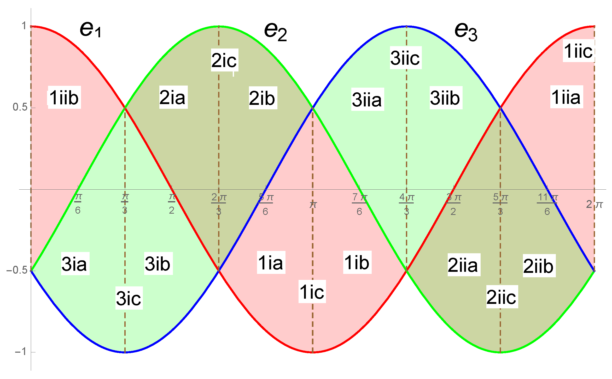
the rigid body is the most asymmetric one: one inertia parameter is zero, and the other two inertia parameters have the same absolute value but opposite signs. Figure 1 shows the inertia parameters as a function of $\kappa$.

These special values of $\kappa$ split the interval $[0,2\pi )$ in twelve disjoint open subintervals. For the values of $\kappa \in [0,2\pi )$, we can continuously cover all the possible asymmetries of the rigid body: symmetrical top ($\kappa \in K_s$) and asymmetrical top ($\kappa \notin K_s$, including the most asymmetrical tops $\kappa \in K_a$), with all the possible ordering of the $e_i$’s parameters, as it is shown in the Figure 1; of course, instead of the inverse inertia matrix ${\mathbb{I}}^{-1}$, we are using the dimensionless matrix $\mathbb{E}=diag\{e_1,e_2,e_3\}$.

The transition from three real inertia moments to a single asymmetry parameter and the conversion of the ratio $E/L^2\in \mathbb{R}$ into the energy-momentum parameter $e_0$ have allowed us to reduce all case studies to only two bounded independent parameters, namely $\kappa$ and $e_0$. For $\kappa$ taking continuous values within its domain $[0,2\pi )$, we naturally obtain the six possible permutations of the three inertia parameters, ranging from symmetric rigid bodies (treated as subsections (c) in all the studied cases, where $\kappa$ is a multiple of $\pi /3$), and notably, to the most asymmetric cases (when one inertia parameter vanishes, if $\kappa$ is an odd multiple of $\pi /6$).

Special cases take place when the rigid body has cylindric symmetry, $\kappa \in K_s$. If $e_i\ne e_j=e_k$ for $i\ne j\ne k$ in the set $\{1,2,3\}$, from (17) we obtain $u_i$ as constant and

$$\begin{array}{ccc}\hfill {\dot{u}}_j& =& \alpha u_k,\hfill \\ \hfill {\dot{u}}_k& =& -\alpha u_j,\hfill \end{array}$$

where $\alpha =(e_i-e_j)u_i$, and the solution is given in terms of circular functions.

The surface of energy (15) and angular momentum (16) define the level surfaces

$$\begin{array}{ccc}\hfill \mathcal{E}& =& \{\mathit{u}\in {\mathbb{R}}^3|{\mathit{u}}^T\mathbb{E}\mathit{u}=e_1{u}_1^2+e_2{u}_2^2+e_3{u}_3^2=e_0\},\hfill \end{array}$$

(20)

$$\begin{array}{ccc}\hfill \mathcal{S}& =& \{\mathit{u}\in {\mathbb{R}}^3|{\mathit{u}}^T\mathit{u}=u_1^2+u_2^2+u_3^2=1\}.\hfill \end{array}$$

(21)

The sphere of angular momentum (21) is a unitary sphere, and the level surface (20), is generically an elliptic hyperboloid instead of the original ellipsoid (5), because at least one inertia parameter is positive and another is negative. Remember that the name energy surface is used for simplicity, and $e_0$ depends also on the square of the angular momentum, see Equation (14). The solution to the dimensionless Euler equation lives at the intersection $\mathcal{E}\cap \mathcal{S}$.

The condition for the intersection between the sphere of angular momentum and the original ellipsoid of energy (7) becomes in these parameters the intersection of the hyperboloid (20) and the unitary sphere (21), with the condition

$$e_{min}\le e_0\le e_{max}.$$

(22)

When $e_0=e_{min}$ or $e_0=e_{max}$, the hyperboloid and the unitary sphere are tangent at only two points.

The geometry of the energy surface (20) depends on the values of $e_0$ and $\kappa$. We have two cases:

I.

$e_0\ne 0$. The energy surface $\mathcal{E}$ has the equation

$$\frac{e_1}{e_0}{u}_1^2+\frac{e_2}{e_0}{u}_2^2+\frac{e_3}{e_0}{u}_3^2=1,$$

(23)

which is either a hyperboloid or a cylinder, depending on the value of the asymmetry parameter:

(i)

$\kappa \notin K_s\cup K_a$. This is the generic case. All the coefficients in (23) are not zero, and

-

If two coefficients are positive, and the other one is negative, let us say $e_i/e_0<0$, then $\mathcal{E}$ is an elliptic hyperboloid of one sheet around the axis $u_i$.

-

If two coefficients are negative, and the other one is positive, let us say $e_i/e_0>0$, then $\mathcal{E}$ is an elliptic hyperboloid of two sheets around the axis $u_i$.

That two coefficients in (23) are positive or negative depends on the sign $e_0$ and on the intermediate inertia parameter, because the other two always have opposite signs.

(ii)

$\kappa \in K_s$ and two inertia parameters are equal. All the coefficients in (23) are not zero, and

-

If two coefficients have the same positive value, and the other one is negative, let us say $e_i/e_0<0$, then $\mathcal{E}$ is a hyperboloid of revolution of one sheet around the axis $u_i$.

-

If two coefficients have the same negative value, and the other one is positive, let us say $e_i/e_0>0$, then $\mathcal{E}$ is a hyperboloid of revolution of two sheets around the axis $u_i$.

(iii)

$\kappa \in K_a$. A coefficient is zero, let us say $e_i/e_0=0$, and the other two have the same absolute value but opposite signs. This is a hyperbolic cylinder with cylindrical axis $u_i$.

II.

$e_0=0$. The energy surface $\mathcal{E}$ has the equation

$$e_1{u}_1^2+e_2{u}_2^2+e_3{u}_3^2=0,$$

(24)

which is either a cone or two intersecting planes, depending on the value of the asymmetry parameter:

(i)

$\kappa \notin K_s\cup K_a$. All the coefficients in (24) are not zero. If two coefficients have the same sign, and the other the opposite one, let us say $e_i$. $\mathcal{E}$ is an elliptic cone around the axis $u_i$.

(ii)

$\kappa \in K_s$. All the coefficients in (24) are not zero: two coefficients have the same value and sign, and the other has the opposite sign, let us say $e_i$, then $\mathcal{E}$ is a circular cone around the axis $u_i$.

(iii)

$\kappa \in K_a$. Then some inertia parameter vanishes, let us say $e_i=0$, and $\mathcal{E}$ are two planes intersecting along the $u_i$ axis.

The solution of (17) for asymmetric rigid bodies is well known in terms of elliptic Jacobi functions, see for instance [33,34], and they live at the intersection of the unitary sphere (6) and the hyperboloid of energy (5).

In the next section, we will take a different approach. We will explicitly find the trajectory equation as the solution to the Euler equations in a reduced two-dimensional space, where the solution depends on trigonometric functions of a cylindric angle $\psi$. The geometry of the solutions is related with the hyperboloids previously characterized in terms of the asymmetry parameter $\kappa$ and the energy parameter $e_0$.

3. The Explicit Solution for the Trajectory Equation

We write the dimensionless Euler Equation (17) in the abbreviated form

$$\begin{array}{ccc}\hfill {\dot{u}}_1& =& \left(e_3-e_2\right)u_2{u}_3=a{u}_2{u}_3,\hfill \\ \hfill {\dot{u}}_2& =& \left(e_1-e_3\right)u_1{u}_3=b{u}_1{u}_3,\hfill \\ \hfill {\dot{u}}_3& =& \left(e_2-e_1\right)u_1{u}_2=c{u}_1{u}_2,\hfill \end{array}$$

(25)

where the coefficients a, b and c are the differences between the inertia parameters, which satisfies $a+b+c=0$ and can be written in different ways

$$\begin{array}{ccc}\hfill a& =& e_3-e_2=-\sqrt{3}\sin \left(\kappa \right)=\sqrt{3}\cos (\kappa +\pi /2),\hfill \end{array}$$

(26)

$$\begin{array}{ccc}\hfill b& =& e_1-e_3=\frac{1}{2}\left(\sqrt{3}\sin \kappa +3\cos \kappa \right)=\sqrt{3}\cos (\kappa -\pi /6),\hfill \end{array}$$

(27)

$$\begin{array}{ccc}\hfill c& =& e_2-e_1=\frac{1}{2}\left(\sqrt{3}\sin \kappa -3\cos \kappa \right)=-\sqrt{3}\cos (\kappa +\pi /6).\hfill \end{array}$$

(28)

We expect these differences of inertia parameters to be present in the solution.

We will introduce cylindrical coordinates for distinguish three possible cases depending on the symmetry axis of the cylindrical coordinates. Then we will solve the Euler Equation (17) eliminating the time $\tau$ to find the trajectory equation parametrized with a cylindric angle $\psi$. In what follows, we assume $r\ge 0$.

In Figure 1, a summary of all the cases and subcases is shown.

• Case 1. Cylindric coordinates $(u_1,r,\psi )$ around the $u_1$ axis

$$u_1=u_1,u_2=r\cos \psi ,u_3=r\sin \psi .$$

(29)

Equation (25) become

$$\begin{array}{cc}\hfill \dot{r}=& {\displaystyle \frac{u_2\dot{u_2}+u_3\dot{u_3}}{r}}=(b+c)r{u}_1\sin \psi \cos \psi ,\hfill \\ \hfill \dot{\psi }=& {\displaystyle \frac{u_2\dot{u_3}-u_3\dot{u_2}}{r^2}}=u_1\left(c{\cos }^2\psi -b{\sin }^2\psi \right),\hfill \\ \hfill \dot{u_1}=& a{r}^2\sin \psi \cos \psi .\hfill \end{array}$$

(30)

Note that

$$\dot{r}=-\frac{{\dot{u}}_1}{r}{u}_1,\mathrm{i}.\mathrm{e}.,r\dot{r}+u_1{\dot{u}}_1=0,$$

and we have the first integral

$$u_1^2+r^2=const.,$$

where $r^2=u_2^2+u_3^2$, which is the conservation of the norm of the angular momentum given in (21)

$$u_1^2+r^2=1.$$

(31)

To solve the equations of motion (30), we change to the independent variable $\psi$, reducing the differential system in one dimension

$$\begin{array}{ccc}\hfill r^{\prime }\left(\psi \right)& =& \frac{dr\left(\psi \right)}{d\psi }=\frac{\dot{r}}{\dot{\psi }}=\frac{r\left(\psi \right)(b+c)\sin \psi \cos \psi }{c{\cos }^2\psi -b{\sin }^2\psi },\hfill \end{array}$$

(32)

$$\begin{array}{ccc}\hfill u_1^{\prime }\left(\psi \right)& =& \frac{d{u}_1\left(\psi \right)}{d\psi }=\frac{\dot{u_1}}{\dot{\psi }}=\frac{a{r}^2\left(\psi \right)\sin \psi \cos \psi }{u_1\left(\psi \right)\left(c{\cos }^2\psi -b{\sin }^2\psi \right)}.\hfill \end{array}$$

(33)

These are the trajectory differential equations in the independent variable $\psi$. Now the system is non-autonomous in a reduced two-dimensional space $(r,u_1)$. In order that these equations be well defined, the denominators of (32) and (33) must be different from zero for all $\psi$. We assume that

$$u_1\left(\psi \right)\ne 0\mathrm{and}bc<0,$$

(34)

and also $r<1$ by (31). Critical points take place when $r=0$ at the points $(u_1,u_2,u_3)=(\pm 1,0,0)$ and they will be studied in the next section. The condition $bc<0$ implies that

$$\kappa \in (2\pi /3,4\pi /3)\cup (-\pi /3,\pi /3),$$

which means that $e_1$ is the smallest or the greatest of the three inertia parameters.

The differential Equation (32) is separated and can be integrated explicitly. Once we have $r\left(\psi \right)$, we can substitute it into Equation (33) and solve it explicitly, or we use the first integral (31) to obtain $u_1\left(\psi \right)$. Integrating (32) we have

$$r\left(\psi \right)=\sqrt{\frac{2H}{c-b+(b+c)\cos \left(2\psi \right)}},$$

(35)

and for $u_1$

$$u_1\left(\psi \right)=\pm \sqrt{1-r^2\left(\psi \right)},$$

(36)

where $2H$, the other first integral, depends on the initial conditions. Factor 2 is convenient as will be seen ahead.

The solutions $r\left(\psi \right)$ and $u_1\left(\psi \right)$ are well defined if (34) is satisfied, and they are periodic functions with period $\pi$. The factor 2 in the argument of the cosine function is due to the invariance of the solution under $\psi \to \psi +\pi$, $(u_1,u_2,u_3)\to (u_1,-u_2,-u_3)$. In other words, the two points $(u_1,u_2,u_3)$ and $(u_1,-u_2,-u_3)$ are on the same solution.

The first integral $2H$ can be easily calculated, and it must be consistent with (20). From (35) and (29), we have

$$\begin{array}{ccc}\hfill 2H& =& (c-b)(u_2^2+u_3^2)+(b+c)r^2({\cos }^2\psi -{\sin }^2\psi )\hfill \\ & =& 2c{u}_2^2-2b{u}_3^2,\hfill \end{array}$$

and using the definitions of b and c, (27) and (28), and the first integral (31) we obtain

$$\begin{array}{ccc}\hfill H& =& e_1{u}_1^2+e_2{u}_2^2+e_3{u}_3^2-e_1(u_1^2+u_2^2+u_3^2)\hfill \\ & =& e_1{u}_1^2+e_2{u}_2^2+e_3{u}_3^2-e_1=const.,\hfill \end{array}$$

then

$$e_1{u}_1^2+e_2{u}_2^2+e_3{u}_3^2=e_0=const.,$$

which is the hyperboloid of energy (20). Then, H and the energy parameter $e_0$ are related by

$$H=e_0-e_1.$$

(37)

We want to relate the first integral H with the values of $r\left(0\right)$ and $r(\pi /2)$. If we denote $r_0=r\left(0\right)$ and $r_{\pi /2}=r(\pi /2)$, from (35) with $\psi =0$ we have

$$H=c{r}_0^2=-b{r}_{\pi /2}^2,$$

In this way, we have that the distances to the cylindrical axis along $u_2$ and $u_3$ are

$$r_0^2=\frac{e_0-e_1}{e_2-e_1},r_{\pi /2}^2=\frac{e_0-e_1}{e_3-e_1},$$

(38)

respectively, where $0<r_0^2<1$ and $0<r_{\pi /2}^2<1$. Thus, we have the relations

$$0<\frac{e_0-e_1}{e_2-e_1}<1,0<\frac{e_0-e_1}{e_3-e_1}<1.$$

(39)

From (34), we consider the following two cases.

(i)

If $b<0$ and $c>0$, then $\kappa \in (2\pi /3,4\pi /3)$ and $e_1$ is the smallest inertia parameter. The denominators of (39) are positive, and for $e_0$ we obtain

$$e_1<e_0,e_0<e_2,e_0<e_3,$$

(40)

so that $e_0$ is less than both $e_2$ and $e_3$ in all the interval $\kappa \in (2\pi /3,4\pi /3)$, and if

(a)

$a<0$ then $\kappa \in (2\pi /3,\pi )$, $e_1<e_0<e_3<e_2$.

(b)

$a>0$ then $\kappa \in (\pi ,4\pi /3)$, $e_1<e_0<e_2<e_3$.

(c)

$a=0$ then $\kappa =\pi$ and the body is symmetric such that

$$-1=e_1<e_0<e_2=e_3=\frac{1}{2}.$$

(ii)

If $b>0$ and $c<0$, then $\kappa \in (-\pi /3,\pi /3)$ and $e_1$ is the greatest inertia parameter. The denominators of (39) are negative, and for $e_0$ we obtain

$$e_1>e_0,e_0>e_2,e_0>e_3,$$

(41)

so that $e_0$ is greater than both $e_2$ and $e_3$ in all the interval $\kappa \in (-\pi /3,\pi /3)$, and if

(a)

$a>0$ then $\kappa \in (-\pi /3,0)$, $e_2<e_3<e_0<e_1$.

(b)

$a<0$ then $\kappa \in (0,\pi /3)$, $e_3<e_2<e_0<e_1$.

(c)

$a=0$ then $\kappa =0$ and the body is symmetric satisfying

$$-\frac{1}{2}=e_3=e_2<e_0<e_1=1.$$

These cases and conditions on $e_1,e_2,e_2,$ and $e_0,$ are shown in the Figure 1 as 1ia, 1ib, 1ic and 1iia, 1iib, 1iic.

As $c-b=-3e_1$ and $b+c=e_2-e_3$, the solutions (35) and (36) in terms of the inertia and energy parameters are

$$\begin{array}{cc}\hfill r\left(\psi \right)=& \sqrt{{\displaystyle \frac{2(e_0-e_1)}{-3e_1+(e_2-e_3)\cos \left(2\psi \right)}}},\hfill \\ \hfill u_1\left(\psi \right)=& \pm \sqrt{1-r^2\left(\psi \right)},\hfill \end{array}$$

(42)

where $e_0$ satisfies (40) or (41). As a function of the asymmetry parameter $\kappa$, Equation (13) yields

$$\begin{array}{c}\hfill r\left(\psi \right)=\sqrt{{\displaystyle \frac{2(e_0-\cos \kappa ))}{-3\cos \kappa +\sqrt{3}\sin \kappa \cos \left(2\psi \right)}}},\end{array}$$

(43)

and

$$u_1\left(\psi \right)=\pm \sqrt{1-r^2\left(\psi \right)},$$

which only depend on the two constant parameters $\kappa$ and $e_0$.

In the special symmetric case (1i c) with $\kappa =\pi \in K_s$, the solutions are reduced to

$$r=\sqrt{\frac{2}{3}(1+e_0)},u_1=\pm \sqrt{\frac{1}{3}(1-2e_0)},(\kappa =\pi )$$

which are two circles perpendicular to the $u_1$ axis with the center at $(u_1,0,0)$ and radio r. In the case (1ii c) with $\kappa =0\in K_s$, the corresponding values are

$$r=\sqrt{\frac{2}{3}(1-e_0)},u_1=\pm \sqrt{\frac{1}{3}(1+2e_0)},(\kappa =0).$$

Finally, from (38) and (29) at $\psi =0$ and $\psi =\pi /2$, the trajectory crosses the planes $u_3=0$ and $u_2=0$, at the points

$$\begin{array}{cc}\hfill {(u_1,u_2,u_3)}_{\psi =0}=& \left(\pm \sqrt{{\displaystyle \frac{e_2-e_0}{e_2-e_1}}},\sqrt{{\displaystyle \frac{e_0-e_1}{e_2-e_1}}},0\right),\hfill \\ \hfill {(u_1,u_2,u_3)}_{\psi =\pi /2}=& \left(\pm \sqrt{{\displaystyle \frac{e_3-e_0}{e_3-e_1}}},0,\sqrt{{\displaystyle \frac{e_0-e_1}{e_3-e_1}}}\right),\hfill \end{array}$$

respectively, such that either (40) or (41) is satisfied.

• Case 2. Cylindric coordinates $(u_2,r,\psi )$ around the $u_2$ axis

$$u_1=r\sin \psi ,u_2=u_2,u_3=r\cos \psi .$$

(44)

The Euler Equation (25) becomes

$$\begin{array}{cc}\hfill \dot{r}=& {\displaystyle \frac{u_1\dot{u_1}+u_3\dot{u_3}}{r}}=(a+c)r{u}_2\sin \psi \cos \psi ,\hfill \\ \hfill \dot{\psi }=& {\displaystyle \frac{u_3\dot{u_1}-u_1\dot{u_3}}{r^2}}=u_2\left(a{\cos }^2\psi -c{\sin }^2\psi \right),\hfill \\ \hfill \dot{u_2}=& b{r}^2\sin \psi \cos \psi .\hfill \end{array}$$

Now $r\dot{r}+u_2{\dot{u}}_2=0$ gives the first integral

$$u_2^2+r^2=const.,$$

where $r^2=u_1^2+u_3^2$, which is the conservation of the norm of the angular momentum (21), i.e.,

$$u_2^2+r^2=1.$$

(45)

The differential system with the independent variable $\psi$ becomes

$$\begin{array}{ccc}\hfill r^{\prime }\left(\psi \right)& =& {\displaystyle \frac{r\left(\psi \right)(a+c)\sin \psi \cos \psi }{a{\cos }^2\psi -c{\sin }^2\psi }},\hfill \end{array}$$

(46)

$$\begin{array}{ccc}\hfill u_2^{\prime }\left(\psi \right)& =& {\displaystyle \frac{b{r}^2\left(\psi \right)\sin \psi \cos \psi }{u_2\left(\psi \right)\left(a{\cos }^2\psi -c{\sin }^2\psi \right)}}.\hfill \end{array}$$

(47)

In order that these equations be well defined, the denominators of (46) and (47) must be different from zero for all $\psi$. We assume that

$$u_2\left(\psi \right)\ne 0,ac<0,$$

(48)

and also $r<1$ by (45). When $r=0$, there are two critical points $(u_1,u_2,u_3)=(0,\pm 1,0)$; they will be studied in the next section. The condition $ac<0$ implies

$$\kappa \in (\pi /3,\pi )\cup (4\pi /3,2\pi ),$$

thus $e_2$ is the smallest or the greatest of the three inertia parameters.

The differential Equation (46) can be integrated explicitly, and with the first integral (45) we obtain $u_2\left(\psi \right)$

$$\begin{array}{ccc}\hfill r\left(\psi \right)& =& \sqrt{\frac{2H}{a-c+(a+c)\cos \left(2\psi \right)}},\hfill \end{array}$$

(49)

$$\begin{array}{ccc}\hfill u_2\left(\psi \right)& =& \pm \sqrt{1-r^2\left(\psi \right)},\hfill \end{array}$$

(50)

the other first integral being H. The solution is invariant under $\psi \to \psi +\pi$, so the points $(u_1,u_2,u_3)$ and $(-u_1,u_2,-u_3)$ belong to the same solution.

Following the same steps as in Case 1, we obtain analogous results with the corresponding permuted indices. For H, we obtain

$$H=e_0-e_2$$

and denoting $r_0=r\left(0\right)$ and $r_{\pi /2}=r(\pi /2)$, we have

$$H=a{r}_0^2=-c{r}_{\pi /2}^2,$$

therefore the square distances to the cylindrical axis $u_2$ along $u_1$ and $u_3$ are given by

$$r_0^2=\frac{e_0-e_2}{e_3-e_2},r_{\pi /2}^2=\frac{e_0-e_2}{e_1-e_2},$$

(51)

respectively, where $0<r_0^2<1$ and $0<r_{\pi /2}^2<1$. Then,

$$0<\frac{e_0-e_2}{e_3-e_2}<1,0<\frac{e_0-e_2}{e_1-e_2}<1.$$

(52)

We have two cases

(i)

If $a<0$ and $c>0$, then $\kappa \in (\pi /3,\pi )$, and $e_2$ is the greatest inertia parameter for all this interval of $\kappa$. The denominators in (52) are negative, and for $e_0$ we obtain

$$e_2>e_0,e_0>e_1,e_0>e_3,$$

(53)

so that $e_0$ is greater than both $e_1$ and $e_3$ in all the interval $\kappa \in (\pi /3,\pi )$, and if

(a)

$b>0$ then $\kappa \in (\pi /3,2\pi /3)$, $e_3<e_1<e_0<e_2$.

(b)

$b<0$ then $\kappa \in (2\pi /3,\pi )$, $e_1<e_3<e_0<e_2$.

(c)

$b=0$ then $\kappa =2\pi /3$ and the body is symmetric and

$$-\frac{1}{2}=e_3=e_1<e_0<e_2=1.$$

(ii)

If $a>0$ and $c<0$, then $\kappa \in (4\pi /3,2\pi )$, and $e_2$ is the smallest inertia parameter in all this interval of $\kappa$. The denominators of (52) are positive, and for $e_0$ we obtain

$$e_2<e_0,e_0<e_1,e_0<e_3,$$

(54)

so that $e_0$ is smaller than both $e_1$ and $e_3$ in all the interval $\kappa \in (4\pi /3,2\pi )$, and if

(a)

$b<0$ then $\kappa \in (4\pi /3,5\pi /3)$, $e_2<e_0<e_1<e_3$.

(b)

$b>0$ then $\kappa \in (5\pi /3,2\pi )$, $e_2<e_0<e_3<e_1$.

(c)

$b=0$ then $\kappa =5\pi /3$ and the body is symmetric and

$$-1=e_2<e_0<e_1=e_3=\frac{1}{2}.$$

These cases and conditions on $e_1,e_2,e_2,$ and $e_0,$ are shown in the Figure 1 as 2ia, 2ib, 2ic and 2iia, 2iib, and 2iic.

As $a-c=-3e_2$ and $a+c=e_3-e_1$, the solutions (49) and (50) in terms of the inertia and energy parameters are

$$\begin{array}{cc}\hfill r\left(\psi \right)=& \sqrt{{\displaystyle \frac{2(e_0-e_2)}{-3e_2+(e_3-e_1)\cos \left(2\psi \right)}}},\hfill \\ \hfill u_2\left(\psi \right)=& \pm \sqrt{1-r^2\left(\psi \right)},\hfill \end{array}$$

(55)

such that $e_0$ satisfies (53) or (54). With (13), the previous solutions can be written in terms of only two parameters $\kappa$ and $e_0$.

In the two symmetrical cases (2i c) and (2ii c), the solutions (55) and are reduced, respectively, to

$$r=\sqrt{\frac{2}{3}(1-e_0)},u_2=\pm \sqrt{\frac{1}{3}(1+2e_0)},(\kappa =2\pi /3)$$

and

$$r=\sqrt{\frac{2}{3}(1+e_0)},u_2=\pm \sqrt{\frac{1}{3}(1-2e_0)},(\kappa =5\pi /3)$$

which are circles perpendicular to the $u_2$ axis with center at $(0,u_2,0)$ and radio r.

Finally, from (51) and (44) at $\psi =0$ and $\psi =\pi /2$, the solution crosses the planes $u_1=0$ and $u_3=0$ at the points

$$\begin{array}{cc}\hfill {(u_1,u_2,u_3)}_{\psi =0}=& \left(0,\pm \sqrt{{\displaystyle \frac{e_3-e_0}{e_3-e_2}}},\sqrt{{\displaystyle \frac{e_0-e_2}{e_3-e_2}}}\right),\hfill \\ \hfill {(u_1,u_2,u_3)}_{\psi =\pi /2}=& \left(\sqrt{{\displaystyle \frac{e_0-e_2}{e_1-e_2}}},\pm \sqrt{{\displaystyle \frac{e_1-e_0}{e_1-e_2}}},0\right),\hfill \end{array}$$

respectively, and either (53) or (54) is satisfied.

• Case 3. Cylindric coordinates around the $u_3$ axis

$$u_1=r\cos \psi ,u_2=r\sin \psi ,u_3=u_3.$$

(56)

The Euler Equation (25) becomes

$$\begin{array}{cc}\hfill \dot{r}=& {\displaystyle \frac{u_1\dot{u_1}+u_2\dot{u_2}}{r}}=(a+b)r{u}_3\sin \psi \cos \psi ,\hfill \\ \hfill \dot{\psi }=& {\displaystyle \frac{u_1\dot{u_2}-u_2\dot{u_1}}{r^2}}=u_3\left(b{\cos }^2\psi -a{\sin }^2\psi \right),\hfill \\ \hfill \dot{u_3}=& c{r}^2\sin \psi \cos \psi .\hfill \end{array}$$

Since $r\dot{r}+u_3{\dot{u}}_3=0$, we have the integral of the norm

$$u_3^2+r^2=1,$$

(57)

and the differential system with the independent variable $\psi$ is

$$r^{\prime }\left(\psi \right)=\frac{r\left(\psi \right)(a+b)\sin \psi \cos \psi }{b{\cos }^2\psi -a{\sin }^2\psi },$$

(58)

$$u_3^{\prime }\left(\psi \right)=\frac{c{r}^2\left(\psi \right)\sin \psi \cos \psi }{u_3\left(\psi \right)\left(b{\cos }^2\psi -a{\sin }^2\psi \right)}.$$

Analogously to the previous cases, we assume that

$$u_3\left(\psi \right)\ne 0,ab<0,$$

(59)

and $r<1$ by (57).

The two critical points take place when $r=0$ at $(u_1,u_2,u_3)=(0,0,\pm 1)$. They will be studied in the next section. The condition $ab<0$ means

$$\kappa \in (0,2\pi /3)\cup (\pi ,5\pi /3),$$

which implies that $e_3$ is the smallest or the greatest of the three inertia parameters.

The Equation (58) is separable, and we obtain

$$r\left(\psi \right)=\sqrt{\frac{2H}{b-a+(a+b)\cos \left(2\psi \right)}},$$

(60)

and

$$u_3\left(\psi \right)=\pm \sqrt{1-r^2\left(\psi \right)}.$$

(61)

Both are well defined if (59) is satisfied. For H in this case, we obtain

$$H=e_0-e_3,$$

If $r_0=r\left(0\right)$ and $r_{\pi /2}=r(\pi /2)$, we have

$$H=b{r}_0^2=-a{r}_{\pi /2}^2,$$

then

$$r_0=\sqrt{\frac{H}{b}},r_{\pi /2}=\sqrt{\frac{H}{-a}},$$

with $0<r_0^2<1$ and $0<r_{\pi /2}^2<1$. Therefore

$$r_0^2=\frac{e_0-e_3}{e_1-e_3},r_{\pi /2}^2=\frac{e_0-e_3}{e_2-e_3},$$

(62)

and

$$0<\frac{e_0-e_3}{e_1-e_3}<1,0<\frac{e_0-e_3}{e_2-e_3}<1.$$

(63)

We have the following two cases:

(i)

If $a<0$ and $b>0$, then $\kappa \in (0,2\pi /3)$ and $e_3$ is the smallest inertia parameter for all this interval of $\kappa$. The denominators in (63) are positive, and for $e_0$ we obtain

$$e_3<e_0{e}_0<e_1,e_0<e_2,$$

(64)

so that $e_0$ is smaller than both $e_1$ and $e_2$ in all the interval $\kappa \in (0,2\pi /3)$, and if

(a)

$c<0$ then $\kappa \in (0,\pi /3)$, $e_3<e_0<e_2<e_1$.

(b)

$c>0$ then $\kappa \in (\pi /3,2\pi /3)$, $e_3<e_0<e_1<e_2$.

(c)

$c=0$ then $\kappa =\pi /3$. The rigid body is symmetric with

$$-1=e_3<e_0<e_1=e_2=\frac{1}{2}.$$

(ii)

If $a>0$ and $b<0$, then $\kappa \in (\pi ,5\pi /3)$, and $e_3$ is the greatest inertia parameter for all this interval of $\kappa$. The denominators in (63) are negative, and for $e_0$ we have

$$e_0<e_3{e}_1<e_0,e_2<e_0,$$

(65)

so that $e_0$ is greater than both $e_1$ and $e_2$ in all the interval $\kappa \in (\pi ,5\pi /3)$, and if

(a)

$c>0$ then $\kappa \in (\pi ,4\pi /3)$, $e_1<e_2<e_0<e_3$.

(b)

$c<0$ then $\kappa \in (4\pi /3,5\pi /3)$, $e_2<e_1<e_0<e_3$.

(c)

$c=0$ then $\kappa =4\pi /3$ and the rigid body is symmetric with

$$-\frac{1}{2}=e_1=e_2<e_0<e_3=1.$$

These cases and conditions on $e_1,e_2,e_2,$ and $e_0,$ are shown in the Figure 1 as 3ia, 3ib, 3ic and 3iia, 3iib, 3iic.

As $b-a=-3e_3$ and $a+b=e_1-e_2$, the solutions (60) and (61) become

$$\begin{array}{cc}\hfill r\left(\psi \right)=& \sqrt{{\displaystyle \frac{2(e_0-e_3)}{-3e_3+(e_1-e_2)\cos \left(2\psi \right)}}},\hfill \\ \hfill u_3\left(\psi \right)=& \pm \sqrt{1-r^2\left(\psi \right)},\hfill \end{array}$$

(66)

where $e_0$ satisfies (64) or (65). With (13), the previous equations can be written in terms of $\kappa$, $e_0$ and of course $\psi$.

In the two special symmetrical cases (3i c) and (3ii c), the solutions (66) are reduced to

$$r=\sqrt{\frac{2}{3}(1+e_0)},u_3=\pm \sqrt{\frac{1}{3}(1-2e_0)},(\kappa =\pi /3)$$

and

$$r=\sqrt{\frac{2}{3}(1-e_0)},u_3=\pm \sqrt{\frac{1}{3}(1+2e_0)},(\kappa =4\pi /3)$$

respectively. They are circles perpendicular to the $u_3$ axis with the center at $(0,0,u_3)$ and radio r.

Finally, from (62) and (56) at $\psi =0$ and $\psi =\pi /2$, the trajectory crosses the planes $u_2=0$ and $u_1=0$ at the points

$$\begin{array}{cc}\hfill ({u_1}_0,{u_2}_0,{u_3}_0)=& \left(\sqrt{{\displaystyle \frac{e_0-e_3}{e_1-e_3}}},0,\pm \sqrt{{\displaystyle \frac{e_1-e_0}{e_1-e_3}}}\right),\hfill \\ \hfill ({u_1}_{\pi /2},{u_2}_{\pi /2},{u_3}_{\pi /2})=& \left(0,\sqrt{{\displaystyle \frac{e_0-e_3}{e_2-e_3}}},\pm \sqrt{{\displaystyle \frac{e_2-e_0}{e_2-e_3}}}\right),\hfill \end{array}$$

respectively, and either (64) or (65) is satisfied.

We have seen that each case has two open disjointed intervals of $\kappa$ (subcases (i) and (ii)), and that the parameter space is divided in six regions where the periodic solutions were found, depending on the value of $e_0$. In Figure 1, we summarize the studied cases. A file Free Rigid Body can be downloaded where the solutions at the intersection of the sphere and hyperboloid can be seen as a function of $\kappa$ and $e_0$; it requires free CDF Wolfram Player.

The boundary of these regions are the special cases where $e_0=e_i$ for some $i=1,2,3$. We study these special cases in the next section.

It must be clear from the previous discussion that the axis of the hyperboloid $\mathcal{E}$, which changes at the values $\kappa \in K_a$ (19), may not be the same as the axis of the cylindrical coordinates used to write the solution, summarized in Figure 1. For instance, for negative $e_0=-0.5$ and $\kappa \in (2\pi /3,4\pi /3)$ (cases (1ia–c)), when $\kappa \in (2\pi /3,5\pi /6)$, $\mathcal{E}$ is a one sheet hyperboloid with axis $u_2$, but the solution has the cylindrical axis $u_1$ (case (1ia)). For $\kappa \in (5\pi /6,7\pi /6)$, $\mathcal{E}$ is a two sheet hyperboloid with axis $u_1$, and the solution has the same cylindrical axis $u_1$ (cases (1ia–c)). For $\kappa \in (7\pi /6,4\pi /3)$, $\mathcal{E}$ is a one sheet hyperboloid with axis $u_3$, but the solution has the cylindrical axis $u_1$ (case (1ib)).

Finally, with the division into six disjoint regions based on the symmetry axis of the cylindrical coordinates to obtain the solutions, we can see that the values of $e_0$ and $\kappa$ are related to the solutions found in each case. The cylindrical symmetry axes where the solutions were calculated coincide with the axes of the larger or smaller inertia parameters, never with the intermediate one. For each value of $\kappa$, there is always an intermediate inertia parameter, which we will refer to as $e_{int}$, and two extremes, denoted as $e_{min}<0<e_{max}$. If the energy parameter $e_0$ satisfies $e_{min}<e_0<e_{int}<e_{max}$, then the solution is expressed in cylindrical coordinates with the cylindrical axis in the direction of $e_{min}$. Conversely, if the energy parameter $e_0$ satisfies $e_{min}<e_{int}<e_0<e_{max}$, then the solution is expressed in cylindrical coordinates with the cylindrical axis in the direction of $e_{max}$. In the symmetric cases, there are two equal inertia parameters, let us say $e_i=e_j$. In this scenario, the different inertia parameter $e_k$ satisfies either $e_k<e_0<e_i=e_j$ or $e_i=e_j<e_0<e_k$. These symmetric cases allow the exchange of the cylindrical axis in the i and j directions for the calculated solution: a parameter $e_i$ that was intermediate for $\kappa$ slightly lower than the value of the symmetric case ($e_i<e_j$), becomes extreme for $\kappa$ slightly greater than in the symmetric case ($e_j<e_i$), and the other one that was extreme becomes intermediate. Of course, the third parameter $e_k$ remains extreme. However, the axis of the cylindrical coordinates for the solution may not necessarily correspond with the axis of the hyperboloid, as we mentioned earlier.

4. The Separatrices

Now we consider the cases in which $e_0$ takes the value of an inertia parameter $e_i$ at the boundary of the regions studied in the previous section. The most simple cases are those in which $r=0$ because the solution reduces to two points. This is confirmed by calculating the limit of the solutions previously found, (42), (55) and (66), when the numerator goes to zero. For instance, in Case 1, we saw that $e_1$ has the smallest or the greatest value of the three inertia parameters, and from (42), if $e_0=e_1$, then $r=0$ and $(u_1,u_2,u_3)=(\pm 1,0,0)$. These are two points on the $u_1$ axis, where the two surfaces (20) and (21) are tangent, as it is expected.

However, in the limit when $e_0$ tends to the inertia parameter with the intermediate value (for a given $\kappa$), the solutions are the separatrix sets given by four semicircles (they are open sets). To see this we substitute the value of $e_0$ in (42), (55) and (66) (Cases 1, 2 and 3, respectively), to the intermediate value of the inertia parameter, as it is indicated in the second column of the next tables.

Case 1 $u_1=\pm \sqrt{1-r^2}$
(i a) $\kappa \in (2\pi /3,\pi )$	$e_0=e_3$, $r=\sqrt{\frac{-3\cos \kappa -\sqrt{3}\sin \kappa }{-3\cos \kappa +\sqrt{3}\sin \kappa \cos 2\psi }}$, $\psi \in \left(-\frac{\pi }{2},\frac{\pi }{2}\right)\cup \left(\frac{\pi }{2},\frac{3\pi }{2}\right)$
(ii a) $\kappa \in (5\pi /3,2\pi )$
(i b) $\kappa \in (\pi ,4\pi /3)$	$e_0=e_2$, $r=\sqrt{\frac{-3\cos \kappa +\sqrt{3}\sin \kappa }{-3\cos \kappa +\sqrt{3}\sin \kappa \cos 2\psi }}$  , $\psi \in (0,\pi )\cup (\pi ,2\pi )$
(ii b) $\kappa \in (0,\pi /3)$
(i c) $\kappa =\pi$	$e_0=e_2=e_3$, $r=1$
(ii c) $\kappa =0$

Case 2 $u_2=\pm \sqrt{1-r^2}$
(i a) $\kappa \in (\pi /3,2\pi /3)$	$e_0=e_1$, $r=\sqrt{\frac{2\left(\cos \left(\kappa \right)-\cos (\kappa -2\pi /3)\right)}{-3\cos (\kappa -2\pi /3)-(\cos \kappa -\cos (\kappa +2\pi /3\left)\right)\cos \left(2\psi \right)}}$,
(ii a) $\kappa \in (4\pi /3,5\pi /3)$	$\psi \in \left(-\frac{\pi }{2},\frac{\pi }{2}\right)\cup \left(\frac{\pi }{2},\frac{3\pi }{2}\right)$
(i b) $\kappa \in (2\pi /3,\pi )$	$e_0=e_3$, $r=\sqrt{\frac{2\left(\cos (\kappa +2\pi /3)-\cos (\kappa -2\pi /3)\right)}{-3\cos (\kappa -2\pi /3)-(\cos \kappa -\cos (\kappa +2\pi /3\left)\right)\cos \left(2\psi \right)}}$,
(ii b) $\kappa \in (5\pi /3,2\pi )$	$\psi \in (0,\pi )\cup (\pi ,2\pi )$
(i c) $\kappa =2\pi /3$	$e_0=e_1=e_3$, $r=1$
(ii c) $\kappa =5\pi /3$

Case 3 $u_3=\pm \sqrt{1-r^2}$
(i a) $\kappa \in (0,\pi /3)$	$e_0=e_2$, $r=\sqrt{\frac{2\left(\cos \right(\kappa -2\pi /3)-\cos (\kappa +2\pi /3\left)\right)}{-3\cos (\kappa +2\pi /3)+\left(\cos \right(\kappa )-\cos (\kappa -2\pi /3\left)\right)\cos \left(2\psi \right)}}$,
(ii a) $\kappa \in (\pi ,4\pi /3)$	$\psi \in \left(-\frac{\pi }{2},\frac{\pi }{2}\right)\cup \left(\frac{\pi }{2},\frac{3\pi }{2}\right)$
(i b) $\kappa \in (\pi /3,2\pi /3)$	$e_0=e_1$, $r=\sqrt{\frac{2\left(\cos \right(\kappa )-\cos (\kappa +2\pi /3\left)\right)}{-3\cos (\kappa +2\pi /3)+\left(\cos \right(\kappa )-\cos (\kappa -2\pi /3\left)\right)\cos \left(2\psi \right)}}$,
(ii b) $\kappa \in (4\pi /3,5\pi /3)$	$\psi \in (0,\pi )\cup (\pi ,2\pi )$
(i c) $\kappa =\pi /3$	$e_0=e_1=e_2$, $r=1$
(ii c) $\kappa =4\pi /3$

In general, assuming that the intermediate value of the inertia parameters is $e_j$, and their ordering is $e_{min}=e_i<e_j<e_k=e_{max}$, $i\ne j\ne k$ in the set $\{1,2,3\}$, if $e_0=e_j$, the solutions are four open semicircles whose boundary points are on opposite sides of the $u_j$ axis. The intersection of the hyperboloid (20) and the unit sphere (21) are two big circles, where the four semicircles lie.

Since the separatrix solution is at the boundary of the two different cases, it can be obtained indistinctly from either of them, as the locus of both solutions coincides, although the domain of $\psi$ is different. For instance, solutions (1ia) are the same locus than (2ib), and (1iia) are the same locus than (2iib), although they come from different limits and symmetry axes. The domain of (1ia) and (1iia) is $\psi \in \left(-\frac{\pi }{2},\frac{\pi }{2}\right)\cup \left(\frac{\pi }{2},\frac{3\pi }{2}\right)$ and of the second one is $\psi \in (0,\pi )\cup (\pi ,2\pi )$.

5. Conclusions

This work was intended to provide an entirely different approach to the torque free Euler equations by mean of the reduction to a cylindrical variable $\psi$ as the new independent variable of the differential system. We used the dimensionless variables and parameters to characterize the rigid body with only two parameters instead of five (three moments of inertia, E and L); they are the asymmetry parameter $\kappa$ and the energy-momentum parameter $e_0$. We made the reduction of the differential system eliminating the time as the independent variable in the Euler equations in dimensionless variables, and we studied the solution and its geometrical aspects by means of continuous deformations dependent on the two independent parameters $\kappa$ and $e_0$. The parameter space was divided into six disjoint regions, whose boundaries are the limit cases where the symmetry axis changes. The solutions depend on where in the six regions—or their boundaries—the values of $e_0$ and $\kappa$ lie in the parameter space, as in each of them an specific symmetry axis is convenient to write the solution. The cases named 1 have the cylindrical axis $u_1$, the cases 2 have the cylindrical axis $u_2$, and the cases 3 have the cylindrical axis $u_3$. Continuously changing the two independent parameters, we obtained the solution $r\left(\psi \right)$ and $u_i\left(\psi \right)$ in cylindrical coordinates, with $u_i$ the cylindrical axis appropriate in each case. The solutions at the boundaries of the regions are the separatrices where there are two symmetry axis, which allows the transition from a symmetry axis to another. Four open circles were found explicitly as a function of $\kappa$, such that $e_0$ takes the value of the intermediate inertia parameter.