Multiscale Entanglement Renormalization Ansatz: Causality and Error Correction

Abstract

Computational complexity reduction is at the basis of a new formulation of many-body quantum states according to tensor network ansatz, originally framed in one-dimensional lattices. In order to include long-range entanglement characterizing phase transitions, the multiscale entanglement renormalization ansatz (MERA) defines a sequence of coarse-grained lattices, obtained by targeting the map of a scale-invariant system into an identical coarse-grained one. The quantum circuit associated with this hierarchical structure includes the definition of causal relations and unitary extensions, leading to the definition of ground subspaces as stabilizer codes. The emerging error correcting codes are referred to logical indices located at the highest hierarchical level and to physical indices yielded by redundancy, framed in the AdS-CFT correspondence as holographic quantum codes with bulk and boundary indices, respectively. In a use-case scenario based on errors consisting of spin erasure, the correction is implemented as the reconstruction of a bulk local operator.

1. Introduction

The quantum advantage refers to a computational complexity scaling with respect to the number of qubits (or in general qudits). For a simulation of a quantum system in a classical computer, this scaling translates into a prohibitively high resource demand. Nevertheless if we relax the most general scenario by focusing on systems characterized by short-range entanglement, tensor network techniques allow us to improve our classical computation capabilities in a stunning way.

The native framework of tensor systems exploits the use of Penrose diagrams [1] in order to pictorially represent tensor indices and their contraction. Tensor diagrams still play a fundamental role, since the optimization of index contraction constitutes a major obstacle in the computational effort minimization required in tensor network algorithms.

A proper formulation of quantum states according to the new ansatz was firstly obtained for one-dimensional spin systems, consisting of matrix product states (MPS) [2] presented in Section 2 and initially used in a completely different framework [3]. In the mathematics literature, the same techniques were already known as Tucker (or tensor train) decompositions [4,5,6,7].

The requirement of new numerical approximation in ground states research was driven by the difference with respect to classical statistical mechanics, where the energy of states can be minimized locally, while this procedure breaks down in a general quantum system. The density matrix renormalization group (DMRG) [8,9] provided an incomparable efficiency by truncating the degrees of freedom endowed with less entanglement according to the Schmidt decomposition. This new recipe for the selection of effective subspaces in iterative renormalization group transformations was completely different with respect to the usual truncation over high energy degrees of freedom used in Wilson’s renormalization.

The extension of tensor network techniques in a higher number of dimensions is still an ongoing development, leading to new tools as the tree tensor network (TTN), able to manage the observable evaluation at different levels of the hierarchy in an optimized manner with respect to tensor contractions by means of orthogonality centers [10]. In Section 3, we will discuss the inclusion of algebraic decay for correlations characterizing phase transitions, which is achieved in MERA [11,12,13,14,15,16], where hierarchical layers include entanglement distillation at the price of introducing loops in the tensor network contraction. Such loops are avoided in augmented TTN [17] if we adopt just one initial layer of disentangler transformations in order to concentrate entanglement within spin blocks.

A widespread application of tensor networks techniques targets lattice gauge theories, concerning the characterization of ground states for both quantum electro-dynamics (QED) [18,19] and non-Abelian interactions [20,21]. Time evolution is included as well through the simulations of QED dynamics concerning string-breaking and scattering phenomena [22,23,24], which are targeted also in noisy intermediate-scale quantum (NISQ) devices [24].

NISQ superconducting devices suffer with respect to the inclusion of entanglement among qubit triplets and more complex structures than pairs [25], thus leading to a short-range entanglement which causes a comparable computational capability of tensor network techniques [26]. This successful application for computational complexity reduction in the quantum framework intertwines with widespread applications in data science [27,28,29,30] and hierarchical tensor geometry [31,32,33]. Hierarchical structures typify in machine learning some information filtering procedures, thus naturally framing tensor network renormalization for these applications, as made by means of wavelets [34]. In general, the relation with statistical analysis is even deeper through the formulation of graphical models in terms of tensor diagrams, built by associating random variables with each node in order to reproduce neural network schemes [35,36,37,38].

In general machine learning procedures pursue the extrapolation of discrete or continuous variables. The last class is generally assessed by means of tomography tools, while the first discrete case is referred to as classification problems, consisting of missing label reconstruction. For our purposes, it is useful to stress that we can equivalently characterize Hamming’s codes, which are commonly used in telecommunications. Logical bits play the same role as labels, protected against errors by a certain redundancy, which ensures our ability to recover their value after a transmission in a noisy channel.

The interface between tensor networks and quantum computing applications is enriched by emerging causal relations in MERA because they naturally frame the associated circuits within an error correction perspective. Hamiltonians are built up in Section 4 in terms of stabilizers in order to define the meaningful code space we wish to study as a ground subspace [39]. This is the case in pure gauge theories for QED toric code [40], as well as including fermionic matter where the Gauss law defines physically meaningful states [18,19,20,21,22,23]. Quantum device realization targets subspace protection against errors as well, like in quantum communications in terms of complexity reduction [41].

In a quantum error correcting code, the subspace we wish to protect by redundancy is referred to logical indices: according to the holographic duality, such inputs live in the bulk, while redundant outputs define the physical lattice at the boundary [42,43] of the holographic codes presented in Section 5. The error correction for a probabilistic spin erasure consists of bulk operator reconstruction, which requires only physical spins at the boundary causally connected with it, as discussed in Section 6.

The main purpose of this paper targets a summary of tensor network methods from both a computational complexity perspective and a coding theory one, bridged together as exemplified by the construction of an anti-de Sitter spacetime disk. Reconstruction of logical labels represents a fruitful topic with respect to possible interfaces among quantum computing, sensing, and data science applications. Simulating hyperbolic spacetime will bring together the aforementioned perspectives, thus leading towards a promising interdisciplinary cross-contamination.

2. MPS in a Nutshell

The simplest scenario required to frame tensor network methods is referred to one-dimensional lattices. Each physical site s of a lattice $\mathcal{L}$ hosts a spin, such that the state $|\psi \rangle \in {\mathcal{H}}_{\mathcal{L}}={⨂}_{s\in \mathcal{L}}{\mathcal{H}}_s$, whose complexity is known to be exponentially hard with respect to the number of spins N, since the Hilbert space dimension is $\dim {\mathcal{H}}_{\mathcal{L}}=2^N$.

In order to face the rapidly increasing demand for computational resources, we need to reduce the number of degrees of freedom by identifying those containing the most relevant amount of information. DMRG numerical methods [8] introduced the efficient cut-off over the Schmidt decomposition components endowed with a coefficient below a certain threshold. This scheme is generalized in terms of MPS [9] based on an iterative reshaping of coefficient arrays and applications of singular value decomposition (SVD).

In general, an SVD corresponds to the Schmidt decomposition for a properly reshaped array of state coefficients:

$$|\psi \rangle =\sum _{s_1,\dots ,s_N}{c}^{s_1,\dots ,s_N}|s_1,\dots ,s_N\rangle ,$$

(1)

depending on the chosen bipartition of the lattice, uniquely determined in the one-dimensional case

$$c^{s_1,\dots ,s_N}⟶c^{(s_1,\dots ,s_{\mathcal{l}}),(s_{\mathcal{l}+1},\dots ,s_N)}=\sum _{a_{\mathcal{l}}}{U}_{a_{\mathcal{l}}}^{(s_1,\dots ,s_{\mathcal{l}})}{\Lambda }^{a_{\mathcal{l}},a_{\mathcal{l}}}{\left(V^{†}\right)}_{a_{\mathcal{l}}}^{(s_{\mathcal{l}+1},\dots ,s_N)},$$

(2)

where $\Lambda$ is a diagonal matrix containing Schmidt coefficients (or singular values) ${\lambda }_{a_{\mathcal{l}}}$. Physical indices grouped within parenthesis, i.e., $(\dots )$, are in general referred to matrix unfolding for tensors [6], such that by introducing the conventional MPS notation used in Figure 1 with rank−3 tensors $A_{a_{\mathcal{l}}}^{1,(s_1,\dots ,s_{\mathcal{l}})}=U_{a_{\mathcal{l}}}^{(s_1,\dots ,s_{\mathcal{l}})}$ and $B_{a_{\mathcal{l}}}^{(s_{\mathcal{l}+1},\dots ,s_N),1}={\left(V^{†}\right)}_{a_{\mathcal{l}}}^{(s_{\mathcal{l}+1},\dots ,s_N)}$

$$|\psi \rangle =\sum _{s_1,\dots ,s_N}\sum _{a_{\mathcal{l}}}{A}_{a_{\mathcal{l}}}^{1,(s_1,\dots ,s_{\mathcal{l}})}{\Lambda }^{a_{\mathcal{l}},a_{\mathcal{l}}}{B}_{a_{\mathcal{l}}}^{(s_{\mathcal{l}+1},\dots ,s_N),1}|s_1,\dots ,s_N\rangle =\sum _{a_{\mathcal{l}}}{\lambda }_{a_{\mathcal{l}}}{|a\rangle }_{a_{\mathcal{l}}}{|b\rangle }_{a_{\mathcal{l}}},$$

(3)

with ${|a\rangle }_{a_{\mathcal{l}}}={\sum }_{s_1,\dots ,s_{\mathcal{l}}}{A}_{a_{\mathcal{l}}}^{1,(s_1,\dots ,s_{\mathcal{l}})}|s_1,\dots ,s_{\mathcal{l}}\rangle$ and ${|b\rangle }_{a_{\mathcal{l}}}={\sum }_{s_{\mathcal{l}+1},\dots ,s_N}{B}_{a_{\mathcal{l}}}^{(s_{\mathcal{l}+1},\dots ,s_N),1}|s_{\mathcal{l}+1},\dots ,s_N\rangle$.

The reason underlying the dummy index in both rank − 3 tensors is related to our choice of an open boundary condition for simplicity. Indeed, we can consider Equation (3) as a first iterative step by imposing $\mathcal{l}=1$ and reshaping

$$c^{a_1,(s_2,\dots ,s_N)}={\Lambda }^{a_1,a_1}{B}_{a_1}^{(s_2,\dots ,s_N),1}⟶c^{(a_1,s_2),(s_3,\dots ,s_N)}=\sum _{a_2}{U}_{a_2}^{(a_1,s_2)}{\Lambda }^{a_2,a_2}{\left(V^{†}\right)}_{a_2}^{(s_3,\dots ,s_N)},$$

(4)

with $A_{a_2}^{s_2,a_1}=U_{a_2}^{(a_1,s_2)}$, named left-normalized matrix because of left-eigenvectors contained in $U_{a_2}^{(a_1,s_2)}$ such that ${\sum }_{s_2}{\left(A^{s_2}\right)}^{†}{A}^{s_2}=\mathbb{1}$.

The iteration of the reshaping and SVD sequence up to a new generic site $s_{\mathcal{l}}$ yields

$$|\psi \rangle =\sum _{s_1,\dots ,s_N}\sum _{a_1,\dots ,a_{\mathcal{l}}}{A}_{a_1}^{s_1,1}{A}_{a_2}^{s_2,a_1}\dots A_{a_{\mathcal{l}}}^{s_{\mathcal{l}},a_{\mathcal{l}-1}}{\Lambda }^{a_{\mathcal{l}},a_{\mathcal{l}}}{\left(V^{†}\right)}_{a_{\mathcal{l}}}^{(s_{\mathcal{l}+1},\dots ,s_N)}|s_1,\dots ,s_N\rangle ,$$

(5)

further elaborated by adopting the reshaping

$${\left(V^{†}\right)}_{a_{\mathcal{l}}}^{(s_{\mathcal{l}+1},\dots ,s_N)}⟶c^{(a_{\mathcal{l}},\dots ,s_{N-1}),s_N}=\sum _{a_{N-1}}{U}_{a_{N-1}}^{(a_{\mathcal{l}},\dots ,s_{N-1})}{\Lambda }^{a_{N-1},a_{N-1}}{\left(V^{†}\right)}_{a_{N-1}}^{s_N},$$

(6)

with the introduction of right-normalized matrices $B_{a_{N-1}}^{s_N,1}={\left(V^{†}\right)}_{a_{N-1}}^{s_N}$ because of right-eigenvectors in ${\left(V^{†}\right)}_{a_{N-1}}^{s_N}$ with ${\sum }_{s_N}{B}^{s_N}{\left(B^{s_N}\right)}^{†}=\mathbb{1}$. A mixed-canonical MPS is obtained by iterations:

$$|\psi \rangle =\sum _{s_1,\dots ,s_N}\sum _{a_1,\dots ,a_{N-1}}{A}_{a_1}^{s_1,1}{A}_{a_2}^{s_2,a_1}\dots A_{a_{\mathcal{l}}}^{s_{\mathcal{l}},a_{\mathcal{l}-1}}{\Lambda }^{a_{\mathcal{l}},a_{\mathcal{l}}}{B}_{a_{\mathcal{l}}}^{s_{\mathcal{l}+1},a_{\mathcal{l}+1}}\dots B_{a_{N-2}}^{s_{N-1},a_{N-1}}{B}_{a_{N-1}}^{s_N,1}|s_1,\dots ,s_N\rangle ,$$

(7)

according to the diagrammatic scheme in Figure 1b.

3. From DMRG to MERA

A polynomial growth of computational complexity is obtained by truncating the number of singular values at each step. A constant dimension imposed for virtual indices along links equal to $\chi$ is named bond dimension [10]. It is chosen with respect to residual error given by the sum of squared neglected singular values, affecting the trace of density matrices.

In general, the efficient selection of degrees of freedom is referred to a renormalization group transformation [11]. A block $\mathcal{B}\subset \mathcal{L}$ of neighboring sites is mapped into an effective coarse-grained site $s^{\prime }$ corresponding to a subspace ${\mathcal{S}}_{\mathcal{B}}\subseteq {\mathcal{H}}_{\mathcal{B}}={⨂}_{s\in \mathcal{B}}{\mathcal{H}}_s$. An isometry maps the effective lattice ${\mathcal{L}}^{\prime }$ into the original one $\mathcal{L}$

$$w:{\mathcal{H}}_{s^{\prime }}⟶{\mathcal{H}}_{\mathcal{B}},w^{†}w=\mathbb{1},$$

(8)

in DMRG based on the truncation of spectral decompositions of the reduced density matrix ${\varrho }^{\left[\mathcal{B}\right]}={\mathrm{Tr}}_{\mathcal{L}\setminus \mathcal{B}}|\psi \rangle \langle \psi |$ on $\mathcal{B}$, such that ${\mathcal{S}}_{\mathcal{B}}=\langle |{\varrho }_1\rangle ,\dots ,|{\varrho }_{\chi }\rangle \rangle$. The bond dimension $\chi$ is referred to the eigenvectors endowed with highest eigenvalues in order to express the amount of entanglement between $\mathcal{B}$ and the remaining part of the lattice $\mathcal{L}\setminus \mathcal{B}$:

$$|\psi \rangle \approx \sum _{i=1}^{\chi }{\lambda }_i|{\varrho }_i\rangle \otimes |{\sigma }_i\rangle ,|{\sigma }_i\rangle \in {\mathcal{H}}_{\mathcal{L}\setminus \mathcal{B}},$$

(9)

chosen with respect to a threshold $\epsilon \ll 1$, such that ${\sum }_{i=1}^{\chi }{\lambda }_i^2\ge 1-\epsilon$. According to the technique presented in Section 2, given a block $\mathcal{B}=\{s_1,s_2\}$, we have to properly reshape the coefficient array $c^{(s_1,s_2),(s_3,\dots ,s_N)}$ in order to select singular values ${\lambda }_i$ of an SVD and associated left- and right-eigenvectors, schematically represented in Figure 2a.

DMRG proved high practical value, but it fails to satisfy the condition related to scale-invariant systems as fixed point, because after a sufficiently high number of iterations the effective sites are unaffordably large. MERA eliminates the growth of the effective site Hilbert space dimension such that a scale-invariant system is mapped to a coarse-grained identical one, unveiling a stratification of entanglement in extended systems [11,12].

This new ansatz is represented in Figure 2b, and it is based on reducing the amount of entanglement between $\mathcal{B}$ and $\mathcal{L}\setminus \mathcal{B}$ by deforming the boundaries of the former through a unitary transformation. In the aformentioned example of a block $\mathcal{B}$ composed by two spins $\{s_1,s_2\}$ with $r_1$ and $r_2$ adjacent on the left and right, respectively, we introduce disentanglers

$$\begin{array}{c}\hfill u_1:{\mathcal{H}}_{r_1}\otimes {\mathcal{H}}_{s_1}⟶{\mathcal{H}}_{r_1}\otimes {\mathcal{H}}_{s_1},\end{array}$$

(10)

$$\begin{array}{c}\hfill u_2:{\mathcal{H}}_{s_2}\otimes {\mathcal{H}}_{r_2}⟶{\mathcal{H}}_{s_2}\otimes {\mathcal{H}}_{r_2}.\end{array}$$

(11)

In this way, we reduce short-range entanglement such that a smaller effective rank $\tilde{\chi }<\chi$ is obtained:

$${\varrho }^{\left[\mathcal{B}\right]}={\mathrm{Tr}}_{r_1{r}_2}\left\{{\varrho }^{\left[r_1{s}_1{s}_2{r}_2\right]}\right\},{\tilde{\varrho }}^{\left[\mathcal{B}\right]}={\mathrm{Tr}}_{r_1{r}_2}\left\{(u_1\otimes u_2){\varrho }^{\left[r_1{s}_1{s}_2{r}_2\right]}{(u_1\otimes u_2)}^{†}\right\},$$

(12)

assuming a lattice composed by $N=4$ sites for simplicity. We have to underline that in general, the block $\mathcal{B}$ does not become completely disentangled because only entanglement localized near its boundary can be removed.

Each layer of a MERA consists of disentanglers $U_{\tau }={⨂}_{i=1}^{N_{\tau }}{u}_i$ and isometries $W_{\tau }={⨂}_{i=1}^{N_{\tau }}{w}_i$, where the index $\tau$ identifies in the hierarchical sequence a lattice ${\mathcal{L}}_{\tau }$ with $N_{\tau }$ spins. We denote each step from a coarse-grained level to a finer-grained one as

$$V_{\tau }=U_{\tau }\circ W_{\tau }:{\mathcal{H}}_{{\mathcal{L}}_{\tau }}⟶{\mathcal{H}}_{{\mathcal{L}}_{\tau -1}},$$

(13)

shown in Figure 3, where for increasing $\tau$, we move towards higher layers in the hierarchy.

The evaluation of observable rule optimizations in tensor network contractions are as those made in a TTN by exploiting orthogonality centers [10]. Corresponding to each lattice ${\mathcal{L}}_{\tau }$ in the hierarchy, observables belong to the algebra $\mathfrak{su}\left(2^{N_{\tau }}\right)$. A renormalization map ${\left({\mathcal{E}}^{*}\right)}_{\tau -1}^{\tau }$ lifts an operator ${\mathcal{O}}_{\tau -1}$ into the above layer:

$${\left({\mathcal{E}}^{*}\right)}_{\tau -1}^{\tau }\left[{\mathcal{O}}_{\tau -1}\right]=V_{\tau }^{†}{\mathcal{O}}_{\tau -1}{V}_{\tau }={\mathcal{O}}_{\tau }^{\prime },$$

(14)

thus named the renormalized operator. In general the layer sequence can be framed in a sequence of moments defining a circuit $\mathcal{C}$, where each site is identified with a wire labeled with the same index s. Causal cones consist of sub-circuits ruled by the following partial order relation [12,15]. For the spins subset $S^{\left[\tau \right]}=\{s_1^{\left[\tau \right]},s_2^{\left[\tau \right]},\dots \}\subseteq {\mathcal{L}}_{\tau }$, we consider those bonds for each $s_i^{\left[\tau \right]}\in S^{\left[\tau \right]}$ connecting to other sites $s_{i,1}^{[\tau +1]},s_{i,2}^{[\tau +1]},\dots$ for a causal relation in the past or $s_{i,1}^{[\tau -1]},s_{i,2}^{[\tau -1]},\dots$ in the future. We can introduce causally connected subsets ${\tilde{S}}_i^{[\tau \pm 1]}=\{s_{i,1}^{[\tau \pm 1]},s_{i,2}^{[\tau \pm 1]},\dots \}$ yielding $S^{[\tau \pm 1]}={\bigcup }_i{\tilde{S}}_i^{[\tau \pm 1]}\subseteq {\mathcal{L}}_{\tau \pm 1}$ and by iteration [42]

$${\mathcal{C}}_P^{\left[S^{\left[\tau \right]}\right]}=\bigcup _{k=\tau +1}^{\Theta }{S}^{\left[k\right]},{\mathcal{C}}_F^{\left[S^{\left[\tau \right]}\right]}=\bigcup _{k=0}^{\tau -1}{S}^{\left[k\right]},$$

(15)

for the causal cone in the past or future, respectively, where $\Theta =O(logN)$ is the circuit depth because of the tree structure.

The renormalization map into a lattice with fewer spins targets the lift of the observable ${\mathcal{O}}_{\tau -1}$ evaluation from ${\mathcal{L}}_{\tau -1}$ to ${\mathcal{L}}_{\tau }$ by considering sites causally connected in the coarse-grained lattice with those interested by the observable action in the finer-grained one:

$$|\langle {\psi }_{\tau -1}\left|{\mathcal{O}}_{\tau -1}\right|{\psi }_{\tau -1}\rangle -\langle {\psi }_{\tau }\left|{\mathcal{O}}_{\tau }\right|{\psi }_{\tau }\rangle |\le \epsilon .$$

(16)

The sites interested by the evaluation in a lower hierarchical layer can be referred to non-adjacent spin blocks, like in the case of correlations, where we may consider the product of a local observable measured in different regions in order to study a ground state near to a quantum criticality. MERA encodes more efficiently this information since it supports algebraic decay of correlations.

For two sites, $s_1$ and $s_2$, separated by a distance r in the physical lattice ${\mathcal{L}}_0$, the corresponding causal cones ${\mathcal{C}}^{\left[s_1\right]}$ and ${\mathcal{C}}^{\left[s_2\right]}$ reach a block of contiguous sites at ${\mathcal{L}}_{\overline{\tau }}$, where $\overline{\tau }={log}_{2}r$. In order to compute ${\varrho }^{\left[s_1{s}_2\right]}$ from ${\varrho }_{\overline{\tau }}$, we use a sequence $\{{\varrho }_{\overline{\tau }},\dots ,{\varrho }_2,{\varrho }_1,{\varrho }^{\left[s_1{s}_2\right]}\}$, that requires $O(logr)$ transformations. In a scale-invariant critical ground state, each of these transformations reduces correlations by a constant factor $z<1$, such that the algebraic decay of correlations is obtained:

$$C_2(s_1,s_2)=\mathrm{Tr}\left\{{\varrho }^{\left[s_1{s}_2\right]}{a}^{\left[s_1\right]}{b}^{\left[s_2\right]}\right\}\approx z^{logr}=r^{-q},$$

(17)

where $q=log\frac{1}{z}>0$ [11,12].

4. Encoding by Redundancy

Classical error correction schemes based on data replication cannot be translated straightforwardly into NISQ devices because of the no-cloning theorem. Quantum error correction exploits encoding maps able to establish a one-to-one correspondence between the logical qubits we need to protect from errors and a subspace, named code space, in a higher dimensional Hilbert space obtained by introducing some ancillary qubits [39]. A simple example of qubit redundancy consists of a single logical qubit $|\psi \rangle =\alpha |0\rangle +\beta |1\rangle$, with ${\left|\alpha \right|}^2+{\left|\beta \right|}^2=1$, mapped into a two-dimensional code space by means of the encoding

$$\mathcal{E}\left[|\psi \rangle \right]=CNOT|\psi \rangle \otimes |0\rangle =\alpha |00\rangle +\beta |11\rangle ,$$

(18)

where the ancilla represents the $CNOT$ target qubit, while the control one is referred to $|\psi \rangle$. Remaining states $\{|01\rangle ,|10\rangle \}$ span the error subspace, which could be partially populated during the elaboration of $\mathcal{E}\left[|\psi \rangle \right]$ by a certain circuit. The detection of such events is implemented by measuring $Z\otimes Z$, which is said to stabilize the logical qubit since

$$Z\otimes Z\mathcal{E}\left[|\psi \rangle \right]=Z\otimes Z(\alpha |00\rangle +\beta |11\rangle )=(+1)\mathcal{E}\left[|\psi \rangle \right],$$

(19)

thus named the stabilizer measurement, with any bit-flip error lying in the $(-1)$-eigenspace.

In general, a stabilizer code takes into account K logical qubits $|{\psi }_{\mathcal{l}}\rangle$, with $\mathcal{l}=1,\dots ,K$, and N physical qubits obtained by redundancy encoding $\mathcal{E}$, whose Pauli group ${\mathcal{G}}_N$ is defined as the set of all operators formed by tensor products of matrices in

$$\{\pm \mathbb{1},\pm \mathrm{i}\mathbb{1},\pm X,\pm \mathrm{i}X,\pm Y,\pm \mathrm{i}Y,\pm Z,\pm \mathrm{i}Z\}.$$

(20)

Stabilizers define an Abelian subgroup

$${\mathcal{S}}_N=\{P_i\in {\mathcal{G}}_N:P_i\mathcal{E}\left[|{\psi }_{\mathcal{l}}\rangle \right]=(+1)\mathcal{E}\left[|{\psi }_{\mathcal{l}}\rangle \right]\forall \mathcal{l}\wedge [P_i,P_j]=0\forall (i,j)\},$$

(21)

where any product $P_i{P}_j$ is a stabilizer because the property $P_i{P}_j|{\psi }_{\mathcal{l}}\rangle =(+1)P_i|{\psi }_{\mathcal{l}}\rangle =(+1)|{\psi }_{\mathcal{l}}\rangle$ holds true. In the error detection process, the set of $M=N-K$ measured stabilizers have to define a minimal set:

$${\mathcal{S}}_N=\langle G_1,G_2,\dots ,G_M\rangle ,$$

(22)

such that any element $G_i$ cannot be obtained as a product among remaining elements.

4.1. Ising Model

In order to frame a MERA in a quantum error-correcting code, we have to consider the top layer $\Theta$ with K logical qubits as the circuit input and the bottom layer as the output with N physical qubits, such that the encoding map reads

$$V=V_1\dots V_{\Theta }:{\mathcal{H}}_{{\mathcal{L}}_{\Theta }}={\left({\mathbb{C}}^2\right)}^{\otimes K}⟶{\mathcal{H}}_{{\mathcal{L}}_0}={\left({\mathbb{C}}^2\right)}^{\otimes N},$$

(23)

with the action over states $\mathcal{E}\left[\varrho \right]=V\varrho V^{†}$ consisting of an isometric quantum channel, with a dual channel referred to the renormalization map ${\mathcal{E}}^{*}$. Each isometry is endowed with a unitary extension $w|\psi \rangle =U_w(|\psi \rangle \otimes |\phi \rangle )$, yielding a unitary quantum circuit of depth $\Theta$ and width N, called the unitary extension of the MERA [14,15].

A simple example consists of the Ising model without an external field over a one-dimensional lattice with periodic boundary conditions:

$$\mathcal{H}=-\sum _{x=0}^{N-1}{Z}_x{Z}_{x+1},$$

(24)

where indices x include the identification $N\equiv 0$. The Hamiltonian is characterized by a two-dimensional degenerate ground subspace, admitting a simple MERA representation with disentanglers equal to the identity, namely a TTN. The non-required disentanglers are caused on a physical ground by the absence of any phase transition because of the missing external field [11].

The ground subspace is a stabilizer code with stabilizer generators ${\left\{Z_x{Z}_{x+1}\right\}}_{x=0}^{N-2}$, so with one term less than those included in Equation (24), because ${\prod }_{x=0}^{N-1}{Z}_x{Z}_{x+1}={\mathbb{1}}^{\otimes N}$ for periodic boundaries, thus missing independence for composition of stablizers by multiplication with neutral element ${\mathbb{1}}^{\otimes N}$. The number of independent generators is $M=N-1$, such that the code space dimension is $2^K=2^{N-M}=2$. The unitary extension of isometries is a $CNOT$, as shown in Figure 4, where a dangling index in the triangle center is referred to the target qubit, i.e., $w|\psi \rangle =CNOT|\psi \rangle \otimes |0\rangle$, chosen as $|0\rangle$ since it is the $(+1)$-eigenstate of Z.

The conjugation by $CNOT$ towards the higher layer yields the renormalized operators we are interested in:

(i)

$CNOT(Z\otimes Z)CNOT=\mathbb{1}\otimes Z$;

(ii)

$CNOT(Z\otimes \mathbb{1})CNOT=Z\otimes \mathbb{1}$.

States encoded by this TTN are $(+1)$-eigenstates of any stabilizer generator, because by exploiting $\left(\mathrm{i}\right)$ for $Z_x{Z}_{x+1}$ referred to the same isometry, we obtain in the higher layer $\mathbb{1}\otimes Z$ with $Z|0\rangle =|0\rangle$ acting like the identity. Instead, for $Z_x{Z}_{x+1}$ related with two isometries, in the form $\mathbb{1}\otimes Z\otimes Z\otimes \mathbb{1}$, we obtain for the first qubit pair $CNOT(\mathbb{1}\otimes Z)CNOT=Z\otimes Z$, while for the second pair we exploit $\left(\mathrm{ii}\right)$, thus obtaining in the higher layer $Z\otimes Z\otimes Z\otimes \mathbb{1}$, where the second operator $Z|0\rangle =|0\rangle$ acts like the identity, namely a coarse-grained spin interaction term. In this way, the number of stabilizer generators is reduced to $\frac{N}{2}-1$ in the higher layer [14].

4.2. Toric Code

Topological codes are based on patching together repeated elements, which generates a size scaling still ensuring stabilizer commutativity. In particular, toric (or equivalently surface) codes are promising for current NISQ devices because they require just nearest-neighbor interaction [39].

Each layer is a two-dimensional lattice, with disentanglers and isometries acting on blocks composed by 16 qubits [13]. The qubits are arranged in an $N\times N$ square lattice with periodic boundary conditions, i.e., a torus, and they occupy edges, such that the total number of qubits is $2N^2$, as physically realized in pure gauge theories for QED with a ${\mathbb{Z}}_2$ discretization [40].

Stabilizer generators consist of star operators, the tensor product of four Pauli X matrices acting on edges connected to the same vertex, and plaquette operators, the tensor product of four Pauli Z matrices acting on edges composing the smallest four-cycle of the lattice. Like the Ising model presented in Section 4.1, we define a Hamiltonian expressed in terms of stabilizer generators:

$$\mathcal{H}=-\sum _{+}{X}_{+}-\sum _{\square }{Z}_{\square },X_{+}=\underset{i\in +}{⨂}{X}_i,Z_{\square }=\underset{i\in \square }{⨂}{Z}_i,$$

(25)

where $X_{+}$ and $Z_{\square }$ are star and plaquette operators, respectively, such that the ground subspace corresponds to the $(+1)$-eigenspace of stabilizers. The lattice periodicity imposes $2N^2-2$ independent generators, thus yielding a code space dimension equal to $2^K=2^{2N^2-(2N^2-2)}=4$, associated with the degrees of freedom of a torus, consisting of non-contractible cycles depicted in Figure 5a.

We need to introduce remaining conjugation by $CNOT$, because of star operators:

(i)

$CNOT(X\otimes X)CNOT=X\otimes \mathbb{1}$;

(ii)

$CNOT(\mathbb{1}\otimes X)CNOT=\mathbb{1}\otimes X$.

where the former motivates the use of $|+\rangle$ as control qubits, the $(+1)$-eigenstate for X. Lattice blocks in Figure 5b–e for renormalization are tilted and the four qubits referred to a vertex of the coarse-grained layer are denoted in black, while twelve qubits included in the finer-grained layer are depicted in red. Half of the latter are stabilized by X and the remaining one by Z: as presented in Section 4.1 for the Ising model, stabilized qubits will take into account interacting terms which disappear in the coarse-grained layer [14], e.g., plaquette terms in panel (b) by exploiting $CNOT$ conjugation introduced in Section 4.1. The same is verified for plaquettes in panels (c,d), whose removal leads to the renormalized lattice with a doubled spacing in panel (e). In the opposite encoding direction, it is proved in [13] that the action of CNOTs, endowed with $|0\rangle$ or $|+\rangle$ as target and control qubits, respectively, defines new plaquettes or vertices including the qubits of the coarse-grained layer involved in aforementioned gates, as shown in Figure 5b–e. Among star operators, like the ones which disappear in the higher level by composing conjugations in panels (b,c) or (d,e), there is one term corresponding to the center of disentanglers in panel (b) just acting like the identity on stabilized $|+\rangle$ qubits in panel (e).

5. Holographic Error Correcting Codes

In the AdS-CFT correspondence, the radial direction can be regarded as a renormalization scale and spacial slices have a hyperbolic geometry, like the exponentially growing MERA tensor network [42]. In general, an anti-de Sitter space is characterized by the metric

$$\mathrm{d}{s}^2=\sum _{i=1}^{\mu }\mathrm{d}{x}_i^2-\sum _{j=1}^{\nu }\mathrm{d}{t}_j^2,$$

(26)

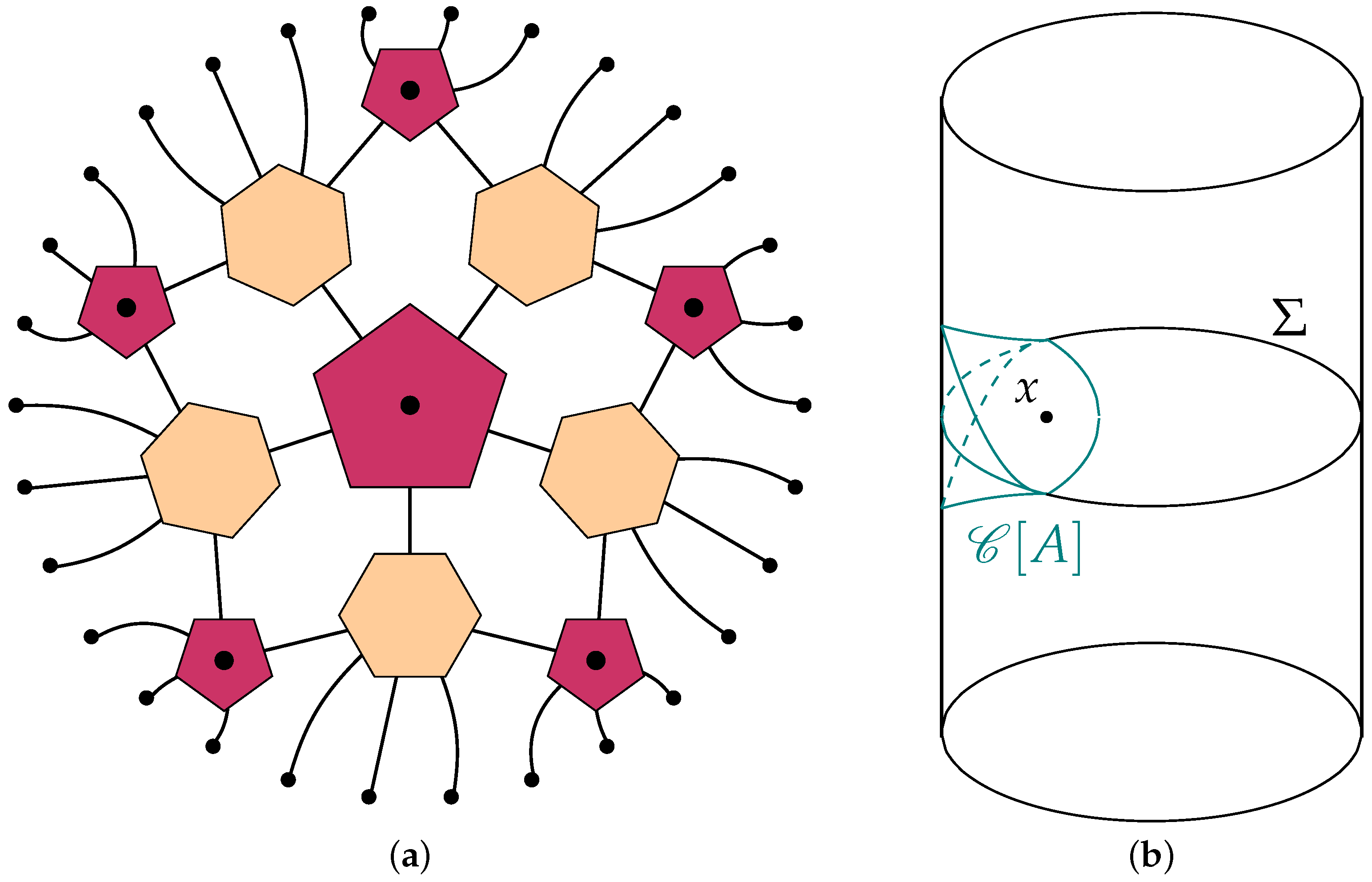
denoted as a $(\mu +\nu )$-dimensional space. We will focus on fixed time slices with periodic boundary of a cylindrical $(1+2)$-dimensional de Sitter space, as represented in Figure 6. Each fixed-time slice is a geometric manifold $\mathsf{\Sigma }$, whose boundary contains the physical degrees of freedom of the spin lattice.

The considered periodic lattice composed of $2N$ qudits, a general case for d-dimensional spins, is described by a pure quantum state $|\psi \rangle$. The set of indices of its coefficients tensor $c^{s_1\dots s_{2N}}$ is divided into a subset A and its complement B, with $\left|A\right|+\left|B\right|=2N$. In this way we map the span of indices in A to the one of those in B. A tensor is perfect if, for any bipartition with $\left|A\right|\le \left|B\right|$, it is proportional to an isometric tensor from A to B, i.e., ${\sum }_b{\left(c^{b{a}^{\prime }}\right)}^{†}{c}^{ba}\propto {\delta }^{a^{\prime }a}$. If c is a unitary transformation when $\left|A\right|=\left|B\right|=N$, then it is perfect. States described by perfect tensors are called absolutely maximally mixed. If $\left|A\right|=1$ and $\left|B\right|=2N-1$, the perfect tensor is an isometric encoding map of a quantum error correcting code, which encodes a single logical spin in a $2N-1$ physical block, with code distance equal to N.

A holographic quantum state is related to a MERA composed of perfect tensors, which cover some geometric manifold $\sum$ associated with a fixed-time slice, where all the interior indices are contracted and physical degrees of freedom are referred to uncontracted legs at the boundary. If there are some open uncontracted legs consisting of bulk indices or logical inputs, like in the case of unitary extensions of isometries, the MERA describes a holographic quantum code, giving rise to an isometric map from bulk to boundary indices.

Holographic states reproduce key properties of the AdS-CFT correspondence, as expressed by the Ryu–Takayanagi formula: in any static state the entropy $S_A$ of a boundary block A at fixed time is

$$S_A=\frac{\mathrm{Area}\left({\gamma }_A\right)}{4G},$$

(27)

where G is the Newton’s gravitational constant and ${\gamma }_A$ is the minimal area bulk surface whose boundary matches $\partial A$. In our simple example, we are dealing with ${\gamma }_A$ consisting of a bulk geodesic, whose length correspond to $\mathrm{Area}\left({\gamma }_A\right)$.

In the discrete tensor network setting, ${\gamma }_A$ is a cut partitioning into two disjoint sets of perfect tensors. Such sets will be denoted with P and Q, as in Figure 7, with some contracted legs along the cut $\gamma$, whose number is called the length of $\gamma$, namely $\left|\gamma \right|$. Let A be a subset of uncontracted physical legs along the boundary corresponding to P, and its complement B is referred to Q, such that the boundary of the cut $\gamma$ is said to match with the boundary of A.

The minimal bulk geodesic ${\gamma }_A$ bounded by A corresponds to the cut $\gamma$ with shortest length. The non-normalized holographic state is expressed in terms of bases $|a\rangle$ and $|b\rangle$ of A and B, respectively

$$|\psi \rangle =\sum _{a,b,\mathcal{l}}{P}^{a\mathcal{l}}{Q}^{b\mathcal{l}}|a\rangle \otimes |b\rangle =\sum _{\mathcal{l}}{|P_{\mathcal{l}}\rangle }_A\otimes {|Q_{\mathcal{l}}\rangle }_B,$$

(28)

where ℓ runs over all possible values of indices contracted along $\gamma$.

The trace over B yields the reduced density operator on A:

$${\varrho }_A=\sum _{\mathcal{l},{\mathcal{l}}^{\prime }}\langle Q_{{\mathcal{l}}^{\prime }}|Q_{\mathcal{l}}\rangle |P_{\mathcal{l}}\rangle \langle P_{{\mathcal{l}}^{\prime }}|,$$

(29)

whose rank is equal at most to $d^{\left|\gamma \right|}$, the number of terms in the sum over contracted indices. The maximal Von Neumann entropy is bounded by choosing the shortest length cut $\gamma ={\gamma }_A$:

$$S_A\le \left|{\gamma }_A\right|logd,$$

(30)

which is saturated if P and Q are isometries from the cut to A and B, respectively. For a simply connected planar tensor network of perfect tensors ruled by a non-positive curvature graph, any connected block A on the boundary saturates the inequality in Equation (30).

The research of a bulk cut ${\gamma }^{*}$ representing a local minimum of the length is implemented by a greedy algorithm. The iterative scheme generates a sequence of cuts $\left\{{\gamma }_{\alpha }\right\}$ bounded by A, with corresponding isometries $\left\{P_{\alpha }\right\}$, such that a local move in the bulk drives the following step from the previous one. Initially, the trivial cut corresponding the boundary block A itself is considered, followed by the inclusion in a new isometry $P_{\alpha +1}$ of a perfect tensor characterized by at least half of its legs contracted with $P_{\alpha }$, as shown in Figure 7. Once the stopping condition is reached, with no more possible local moves, the optimal bulk geodesic ${\gamma }^{*}$ is obtained. Given a connected boundary region A, the set of bulk points reached in the greedy algorithm defines the causal wedge $\mathcal{C}\left[A\right]$, shown in Figure 6b [42].

6. Discussion and Conclusions

Any bulk operator $\varphi \left(x\right)$ referred to a point $x\in \mathcal{C}\left[A\right]$ can be represented as some non-local operators on the boundary region A. The reconstruction of $\varphi \left(x\right)$ is interpreted as correcting spin erasure in B: operators near the bulk center are protected because a large boundary block has to be erased in order to prevent their reconstruction.

Causally connected regions in MERA with a spin block A in the physical lattice establishes the relation with quantum error correction based on the no-cloning theorem. Indeed, the expectation of an observable referred to the physical lattice block A can be reconstructed as the one of an observable lifted by a sequence of isometries and disentanglers: such correspondence is related with holographic AdS-CFT duality between bulk and boundary. The causal relation imposes a condition: if the remaining part of the physical lattice B is not correlated, any spin erasure in the latter does not concern the information shared by the aforementioned observables, the initial and the lifted one. This statement is caused by the no-cloning theorem because it is not possible to clone any information in the remaining part of the lattice as a third party: the information in the bulk lifted observable is protected by any erasure of spins in a product state.

The reconstruction of an operator $\varphi \left(x\right)$ referred to a fixed bulk point changes by moving the block of sites on the boundary: the non-uniqueness of the operator on the boundary leads to the perspective of the bulk operator as a logical one, preserving a code space of the boundary Hilbert space. This code space can be interpreted as the low-energy sector, because local bulk operators correspond to non-local boundary ones.

As a use-case scenario, we consider a probabilistic noise model, where each spin in the boundary is erased with probability p, such that the connected block A breaks into many connected islands. We would like to characterize a code able to correct errors if p is less than a threshold. The greedy algorithm propagates erasure of spins in the boundary towards the bulk center, where local operators cannot be reconstructed if the number of errors exceeds a threshold, since the recovery is not possible if a non-trivial logical operator has support on the erased qudits.

To obtain more resilient codes, we have to modify the holographic code by thinning out the algebra of bulk logical operators, thus reducing the code rate, namely the number of logical qudits over the number of physical ones. A useful strategy consists of alternating tensors with a dangling index with those completely contracted, thus mimicking unitary extensions of MERA, as shown in Figure 6a for the pentagon/hexagon code [42].

A properly defined limit of continuous MERA leads to the study of continuous de Sitter space [15,44,45,46], which is potentially simulated by means of a quantum optics tensor network technique making use of the same real-space renormalization [47].