Dynamical and Probabilistic Approaches to Irreversibility

Abstract

Boltzmann’s H-theorem is considered a great triumph of science. Though some modifications are necessary to adapt it to modern dynamical theories, it is well established that one of its main tenets remains widely accepted: the introduction of probability is a key element in achieving a transition from time-reversible, deterministic dynamical laws at the microscopic level to irreversible laws describing the approach to equilibrium of isolated macroscopic systems. Thus, it is somehow surprising that we still find instances where this subject is labeled as paradoxical and elusive. More remarkable is the fact that this often happens in texts that succeed in presenting Boltzmann’s ideas with clarity. In order to shed light on how probability allows us to go form microscopic reversibility to macroscopic irreversibility, we use numerical results from a two-dimensional lattice gas composed of distinguishable particles. We discuss the roles played by noise, coarse graining, and probability. The simplicity of our model might help the newcomer to this area in better grasping Boltzmann’s fundamental breakthrough.

1. Introduction

In classical mechanics, the fundamental dynamical equations governing the motions of particles have time-reversal symmetry. In principle, these deterministic laws of motion allow us to ascribe a trajectory to any particle as it travels through space, perhaps interacting with a few other particles and boundaries. Conversely, when dealing with a system composed of a very large number of particles, for example, an ideal gas, we are forced to describe its state by using just a few average macroscopic quantities, such as volume, pressure, or temperature, due to our inability to monitor an immense number of degrees of freedom. In this latter case, trying to determine the trajectories of individual particles is not feasible. From a thermodynamic perspective, the evolution of an isolated macroscopic system from a non-equilibrium to an equilibrium state is an irreversible process. That is, there is an arrow of time. Thus, considering the reversible nature of the microscopic laws of motion, we might ask at what point this arrow of time emerges. In 1872, Boltzmann answered this question with his H-theorem, in which he inserted probabilistic arguments. By establishing a kinetic equation, he showed how an isolated multi-particle system tends towards a state of equilibrium, which is where it will remain if left undisturbed [1,2,3,4,5,6,7].

From the very beginning, Boltzmann’s ideas were harshly criticized, most prominently by Loschmidt and Zermelo [3,5,7,8,9,10,11]. However, nowadays, the issue of this reversible-to-irreversible transition is considered mostly settled. For example, in his classical textbook on statistical mechanics, Tolman pointed out that the H-theorem is regarded as one of the greatest achievements of physical science [4]. Thus, it is somehow surprising that adjectives such as paradoxical, elusive, intriguing, etc., are attached to some of the consequences derived from it, even in texts that, in the author’s opinion, succeeded in offering clear explanations of the emergence of irreversibility [3,6].

We must emphasize that in this paper, we embrace the viewpoint that the origin of irreversibility is of a statistical nature. However, as will be discussed in Section 7, there exist other positions in which probability does not play a role in the emergence of an arrow of time.

The main goal of this paper is to present a framework that allows a simple and direct formulation in which the passage from a reversible to an irreversible description of the evolution of a multi-particle system is clear and evident. We will emphasize that the key element in achieving this is the introduction of probability. To this end, in Section 2 we introduce a simple two-dimensional, time-reversible lattice gas model consisting of distinguishable particles. The system evolution from an atypical to a typical configuration, and then backwards upon dynamical inversion, provides us with a setting to discuss apparent irreversibility in Section 3. In Section 4, we present a possible scenario in which the introduction of noise breaks time reversibility, obtaining a dynamical model that is intrinsically irreversible. However, we notice at this point that the resulting entropy is not a monotonically non-decreasing function of time, as required by the second law of thermodynamics (we do not discuss other ideas regarding the emergence of intrinsic irreversibility, such as the proposal of Prigogine and co-workers to modify the microscopic fundamental laws of motion [6,12,13]). In Section 5, we study the configurational entropy of our system from different coarse-grainings. Though the dynamics of our model produces some clearly unrealistic situations, as exemplified by the quasi-periodic behaviors shown in Section 4, in Section 6, we show that it can be used as a tool to demonstrate, in an uncomplicated manner, how the introduction of probability allows us to go from describing the motion of particles with time-reversible dynamics to describing the state of a multi-particle system with monotonically non-decreasing functions of time.

We do not discuss chaos in relation to irreversibility, though in Section 4, we show that the trajectories of our system are unstable under the presence of noise, suggesting a quasi-chaotic behavior.

A quantum-mechanical treatment of the reversible-to-irreversible transition is outside the scope of this paper. References [14,15] are good examples of work that was conducted in this area.

2. Rules of Motion for a Two-Dimensional Lattice Gas of Distinguishable Particles

Let us consider a time-reversible lattice gas model consisting of N distinguishable particles that occupy the sites or nodes of a square lattice. Only horizontal and vertical particle motions are possible. Figure 1 shows, from left to right, four sites with a single particle each. Right, down, left, and up directions are indicated by black, red, green, and blue arrows, respectively (colors are merely a visual aid to identify the direction of a particle). At the upper right section of this lattice, we can see sites with two or more particles. No two particles with same direction can occupy the same site. A site can host up to four particles.

Similar to space, time is a discrete quantity. Every unit time, each particle performs two consecutive steps: translation, followed by clockwise interaction. During translation, a particle moves to an adjacent site according to its direction (if a particle reached an edge of a system, then its velocity direction is rotated by 180° at that time). Particles that are clockwise interact in the following manner: when precisely two particles with opposite directions enter the same site, their directions are clockwise rotated by 90°. Figure 2a shows that, at time t, particles a and b are separated by two length units. At time t + 1, they meet at the site in between (Figure 2b) and rotate 90° clockwise (Figure 2c). Colors change according to the direction–color convention established in Figure 1. Figure 2d shows particle positions at t + 2.

In Figure 3a–c we observe three particles that meet simultaneously at the same site (Figure 3b); in this case, they keep their original directions, since a rotation only occurs when exactly two particles with opposite directions coincide at the same site.

The clockwise interaction dynamics allow us to follow the individual trajectory of every particle, as is made clear by the use of particle labels in Figure 2 and Figure 3. In Figure 4a, we show a 20 × 20–site system with one particle per site at t = 0. The velocity directions were randomly set. The symbol size of a particle at the center was enlarged so that we can easily follow its trajectory. At t = 10, the particle changed its direction after reaching the lower boundary (Figure 4b). Figure 4c shows the same particle at t = 100.

The position and velocity direction of any particle at a given time can be determined if we know the system state at any other past of future time. That is because the dynamics dictated by the clockwise interaction rule are deterministic and time reversible (this point will be made clear when we define dynamical inversion in Section 3).

As described in this section, our model corresponds to an isolated system. That will not be the case when we introduce noise in Section 4.

If we consider indistinguishable particles, as we do in Section 5, our model transforms into the lattice gas model developed by Hardy, Pomeau, and Pazzis [7,16]. We chose to start our discussion with a model with distinguishable particles because at the microscopic level, classical particles are distinguishable.

Other simple models were proposed to clarify the reversible-to-irreversible transition from a probabilistic perspective [17,18,19,20,21]. Kac’s one-dimensional ring model [17,20,21] is perhaps the best known. Conceptually, the two-dimensional lattice gas model presented in Section 2 is as simple as Kac’s ring model. Both describe scenarios in which an arrow of time emerges as we switch from a dynamical to a probabilistic approach, similarly to what Boltzmann achieved in his H-theorem with the assumption of molecular chaos. However, based on the figures and numerical results of the following sections, we argue that our lattice gas displays more realistic behaviors than Kac’s model: (1) Particles spread across the system in a diffusive manner. (2) Instability of trajectories suggests a quasi-chaotic behavior. (3) A meaningful configurational entropy can be calculated. (4) The effects of coarse graining on the evolution of entropy can be studied. (5) Interaction with a heat reservoir can be simulated by the introduction of noise, which destroys time reversibility.

Since time and space are discretized in our model, numerical truncations are not present in our calculations (this is not the case for more realistic models, e.g., ideal gases). This greatly simplifies discussions regarding the roles played by noise, coarse graining, and the introduction of probability in the emergence of irreversibility.

It is difficult to imagine a simpler dynamic for distinguishable particles moving along a two-dimensional lattice than the one presented here. Thus, in extrapolating the results obtained with it to a more realistic and complex scenario, we have to be fully aware of its limitations. For example, the number of configurations that this system can visit is finite. Therefore, any configuration will be re-visited after a certain number of time units (this is known as recurrence time). Except for situations of highly symmetric configurations (see Section 4), the recurrence time is very large, and in most situations we do not have to take it into consideration, since the system evolutions discussed in this paper are for time ranges much smaller than the recurrence time. Along these lines, we might argue that if our universe was reversible but with an exceedingly long recurrence time, it would appear perfectly irreversible to us.

3. Apparent Irreversibility

Before discussing noise and the introduction of probability into the description of the evolution of a system from atypical to typical configurations, in this section, we discuss the concept of apparent irreversibility.

Consider the configuration shown in Figure 5a. At t = 0, every site on the left half of a 50 × 50 site system hosts one particle; the right half is empty. The velocity directions of the 1250 particles are randomly set. Figure 5b–d shows how particles diffuse over the entire system. The system evolves from a special, atypical state (Figure 5a) to a more typical state at t = 500 (Figure 5d). This looks similar to the irreversible diffusive processes that we observe in nature. However, the rules of motions in our system are time reversible: what we observe in the progression of plots of Figure 5a–d is apparent irreversibility [4,6] (in our context, the word apparent is used in the sense of a situation that appears real or true, but that it is not necessarily so). If at t = 500 we performed a dynamical inversion (a process in which we invert the directions of all particles, inverted the order of the translation and interaction steps, and switched the clockwise interaction to a counterclockwise interaction), all particles would return to their original positions, with inverted directions, at t = 1000. This is illustrated by the black curve of Figure 6, where N_L, the number of particles on the left side of the system (1250, initially), is plotted as a function of time. Though a damped oscillatory pattern is observed (a reflection of a ballistic initial behavior of the particles), it is clear that for t < 500, the configuration of the 1250 particles tends toward a more typical distribution where N_L is around 625. After the dynamical inversion at t = 500, N_L traces a mirror image of the behavior observed for t < 500, and it reaches N_L = 1250 at t = 1000.

Because knowing the exact initial configuration is equivalent to knowing the exact configuration at any other time, information is not degraded with time, and thus entropy remains constant, S = 0 (This is similar to a well-known result in statistical mechanics. We can think in terms of an ensemble of Hamiltonian systems. The points in phase space representing their states would behave similar to a fluid. The Liouville’s theorem states that the density of the fluid in the neighborhood of each point, as it travels through phase space, is constant in time. Thus, entropy remains constant, since it is a function of such density. In Section 5, where coarse graining is introduced, we will see that entropy depends on how much information about the system’s configuration we employ in calculating S). Though apparently the system increasingly becomes more disordered with time for t < 500, we saw that the special state at t = 0 can be recovered by dynamical inversion.

Figure 5a–d gives a complete description of the state of the system. When we know all the positions and velocity directions of every particle, we say that we have a micro-description of the system. On the other hand, Figure 6 gives us a macro-description of the state of the system (it describes the state by just one variable: N_L).

4. Noise and Irreversibility

We could think of the system depicted in Figure 5a–d as a simplification of an ideal gas inside a perfectly isolating container that allows for the exchange of neither energy nor particles with the exterior: a system with no contact whatsoever with the rest of the universe. As shown in the previous section, if at time t = 500 we perform on this system a dynamical inversion, we would observe that the more or less evenly distributed particles of Figure 5d would spontaneously collect themselves into the left half of the system at t = 1000 (see black line in Figure 6). If we did not know that the seemingly disordered configuration of Figure 5d was in fact a very special one, we could be quite surprised by the particle crowding at t = 1000. We might call it an atypical event. However, considering that in nature, as far as we know, there are no perfectly isolated systems, we assume that it is extremely unlikely that we will ever observe such atypical behavior; even in a simple toy model such as ours, the system trajectories are very sensitive to any configurational variation, and thus the tiniest perturbation would prevent, with overwhelming probability, the occurrence of such regrouping evolutions. To illustrate this, let us, in addition to the dynamical inversion at t = 500, pick up randomly a single particle and change its direction (think of this as introduction of noise). We will observe that the system does not return to the initial configuration with all particles on the left (N_L = 1250), as shown by the red curve in Figure 6, the amplitude of the oscillations keeps decreasing for t > 500, while N_L approaches a more typical value around 625. That is, the system trajectory described by the black line from t = 500 to 1000 is quite unstable (A simple argument regarding trajectory instability corresponding to an atypical evolution of our simple system goes like this: Consider all of the states that fit the description of particles being more or less evenly spread over the whole system. Of these, only a very small fraction will evolve in the following 500 time units into configurations where all particles are crowded in one half of the system. So, if a particular configuration belongs to this very special group, it is very likely that another one, which differs from the former by the direction or position of a single particle, will not evolve into an atypical crowded situation. Thus, a small variation very likely will destroy a potential particle regrouping).

Another illustration of how easily noise drives our system toward typical states is the following: consider the 20 × 10 site system of Figure 7, in which, again, all particles are initially on the left half, with one particle per site (N_L = 100 at t = 0). This time, all particles are initially pointing to the right, travelling as an ordered group: the black curve of Figure 8 indicates that at t = 0, N_L = 100, whereas N_L = 0 at t = 10. After bouncing at the right border of the system and interacting among themselves, the particles travel mostly toward the left. The black line of Figure 8 illustrates a quasi-periodic behavior for N_L. A more interesting pattern can be observed if the time range of this plot is expanded to 3000 time units, as shown by the black line of Figure 9. Again, if at t = 0 we choose at random one particle and alter its initial direction, we see that the atypical quasi-periodic evolution (black lines of Figure 8 and Figure 9) becomes progressively more typical (fluctuating around N_L = 50), as indicated by both red lines.

Examples such as these suggest that noise can be considered as one of the fundamental factors driving a system into typical configurations, providing nature with an arrow of time [22]. In fact, with the addition of noise, the dynamics of our system became intrinsically irreversible, since its time-reversal property is broken [23]. As explained in the previous section, in the absence of noise, the evolution of our system from atypical to typical configurations is only an apparent irreversible process (It is also possible that a configuration that would not evolve, if left undisturbed, into an atypical one within a short period of time, does precisely that by a small random changes in its configuration. Understandably, this would be a very unlikely event).

5. Indistinguishability, Coarse Graining, and Configurational Entropy

The deterministic rules of motion and the distinguishability of the particles of the lattice gas of Section 2 allows us to determine the position x_i and velocity direction v_i of particle i for t = t + 1 if we know the positions and directions of all N particles at t = t (or at any other past or future time). This determinism can be expressed by two functions X_i and V_i:

x_i(t+1) = X_i({x₁(t), x₂(t), …, x_N(t)}, {v₁(t), v₂(t), …, v_N(t)})

(1)

and

v_i(t+1) = V_i({x₁(t), x₂(t), …, x_N(t)}, {v₁(t), v₂(t), …, v_N(t)}).

(2)

A different situation arises when we are not able to determine the exact state of a system. For example, if we cannot keep track of the identity of each particle (they become indistinguishable to us) but still know all positions and velocity directions, then our model transforms into the lattice gas model of indistinguishable particles proposed by Hardy and co-workers [16]. In this latter model, the meeting of exactly two particles with opposite directions at the same site, at time t, results in two particles leaving the site, at time t+1, in opposite directions that are perpendicular to the original ones. We cannot follow in most cases an individual particle as we did in Figure 4a–c. We have to give up the concept of particle trajectory. Nevertheless, as with the model of Section 2, knowing the state of a system at a given time is equivalent to knowing its state at any other time: the dynamics are deterministic and reversible [7,16].

Imagine that our picture of the microscopic world loses more detail. Now, in addition to being unable of knowing the identity of each particle, suppose that we could not distinguish particle directions (though we were still able to count how many particles reside in each site). Then, we would have a coarse-grained picture. Following a convention introduced in Ref. [7], we say that this coarse-grained description, or c-view, has a coarse-graining index c = 1, because we cannot see details inside an area, or cell, containing a single site. Similarly, we say that c = 2 refers to 2 × 2 sites square cells, and so on.

The information that a c-view gives us about a system with N_c cells (each containing c × c sites) is the number of particles inside each cell, called occupation number. Neither velocity directions nor positions (if c > 1) within the cell are provided. A c-view is specified by the cell occupation numbers (N_c in number) n₁, n₂, …, n_Nc, with n₁ + n₂ + … + n_Nc = N, and N being the total number of particles in the system. Of course, within a cell, particles are considered indistinguishable entities.

We can define a configurational entropy at different space scales by using different c-views. Let Ω be the number of particle configurations compatible with the N_c cell occupation numbers n₁, n₂, …, n_Nc. Then, the c-view entropy can be defined by Boltzmann’s fundamental relation:

$$S^{\left(c\right)}=k_B\ln \left(\mathsf{\Omega }\right),$$

(3)

where k_B is the Boltzmann’s constant. Taking into account the indistinguishability of particles, we have it that [7]:

$$\frac{S^{\left(c\right)}}{k_B}=N_c\ln \left(4c^2\right)!-{\sum }_{I=1}^{N_c}\left\{\mathrm{l}\mathrm{n}{n}_I!+\ln \left(4c^2-n_I\right)!\right\}.$$

(4)

On average, $S^{\left(c\right)}$ increases as a system evolves from an atypical to a typical configuration. The black curve in Figure 10 represents the coarse-grained entropy S^(c=2) as a function of time for the system with the initial configuration depicted in Figure 5a (in Figure 6, the black curve illustrates how N_L evolves from the same initial configuration). As the particles spread over the system (from t = 0 to t = 500), the entropy tends to increase (recall that the prominent damped oscillatory behavior simply reflects a transitory ballistic stage, due to the simplistic rules of motions obeyed by the system). Dynamical inversion occurs at t = 500, and thus the entropy retraces its path and recovers its initial value at t = 1000. As in Figure 6, the red line in Figure 10 represents the entropy for the case where, at the time of the dynamical inversion, noise was introduced by changing the direction of a single particle chosen at random, preventing the return of the system to states of low entropy.

The black curves of Figure 11 and Figure 12 represent the entropy (c = 2) for the system with the initial configuration of Figure 7. As in Figure 8 and Figure 9, which show N_L as a function of time for this system, the black curves represent the entropy in the absence of noise. We see a similar quasi-periodic behavior, this time in entropy, as in Figure 8 and Figure 9. Again, the red curves represents entropy when the direction of a single particle, chosen at random, was altered at t = 0. Noise drives the system to higher entropies over time.

Entropy depends on the amount of detail that we use in describing the state of a system, and thus it is a function of c. Let us illustrate this. In Figure 13, we have a chessboard-like arrangement of particles (t = 0), where half of the 4 × 4 site squares have two particles in each site (32 particles per each square), with directions randomly selected, while the squares of the other half have no particles. We would expect that S would increase with time only if we could study the system with a resolution no larger than the area of the squares. With c = 2 and c = 4 c-views, populated regions can be distinguished from unpopulated ones. In Figure 14 we observe that, as the particles spread along the system, S tends to increase for c = 2 and c = 4 (black and red curves). However, for c = 8 and c = 16, the cells are too big to capture the special (and atypical) initial particle arrangement, and therefore, S does not seem to increase, but merely fluctuates around typical values. Notice that the smaller the coarse-graining index, c, the more information we have about the state of the system and, therefore, the smaller the entropy.

The entropy curves that were so far presented show fluctuations; even the red curve of Figure 10 shows small fluctuations for times close to t = 1000, the stage at which an equilibrium-like situation was reached. Thus, we have that for some times dS/dt < 0, contradicting the second law of thermodynamics. In the next section, we illustrate how, by introducing probabilistic elements into our description of the system time evolution, a monotonically non-decreasing function for S is obtained.

6. A Probabilistic Approach

So far, the c-views (coarse-grained descriptions of a system) that we presented are calculated using an underlying succession of exact states produced by numerical simulations that follow the deterministic rules of motion of Section 2. This is what we call a dynamical approach. Our model, which is an example of a cellular automaton, plays in this paper the role of reality, which can be studied from different perspectives or coarse grainings. Now, we illustrate how we can describe its time evolution, adopting a probabilistic approach.

Let us suppose that we wish to predict the average behavior of a system for which its initial configuration is not fully specified, and that we only know the initial number of particles in each site and have no knowledge about their velocity directions. We could then assume that a particle at site (x, y) at time t can move, at time t + 1, to sites (x + 1, y), (x − 1, y), (x, y + 1), and (x, y − 1) with equal probability (=1/4) (here we refer to an inner site, that is, a site that does not belong to a system edge). Thus, instead of describing the state of a system by specifying particle positions and directions, we can make use of a site particle density ρ_x,y(t), which is now a positive real number within the continuous interval 0 ≤ ρ_x,y ≤ 4 (recall that a site can have up to four particles). For an inner site (x, y), we calculate its particle density at time t+1, ρ_x,y(t+1), as follows:

$${\rho }_{x,y}\left(\mathrm{t}+1\right)=\frac{1}{4}\left[{\rho }_{x-1,y}\left(t\right)+{\rho }_{x+1,y}\left(t\right)+{\rho }_{x,y-1}\left(t\right)+{\rho }_{x,y+1}\left(t\right)\right].$$

(5)

For sites at the edges of a system, we must consider that particles do not cross such limits [7]. By convention, the initial value ρ_x,y(t = 0) corresponds to the particle occupation number (0, 1, 2, 3, or 4) of site (x, y) at t = 0.

In Figure 15a, we show the site particle density, ρ, at t = 0, corresponding to the configuration depicted in Figure 5a, a 50 × 50 site system with one particle at each site on the left half of the system and none for those sites on the right half. Figure 15b,c shows ρ_x,y at times t = 50 and 500, respectively. Black represents ρ = 1 and white represents ρ = 0; values in between are represented by shades of gray.

Likewise, the corresponding site particle densities, ρ, for the initial chessboard configuration of Figure 13 is shown in Figure 16a. Figure 16b–d shows ρ for t = 0, 1, 5, and 10, respectively. In this case, black represents ρ = 2 and white represents ρ = 0; values in between are represented by shades of gray.

In contrast to the situation depicted in Figure 5a–d, the evolutions of the particle density patterns of Figure 15 and Figure 16 are truly irreversible, since as time passes the particle, density becomes increasingly more homogenous across the system (a dynamical inversion is not possible here). As pointed out above, application of Equation (5) implies that we are making a probabilistic prediction about future configurations, starting from incomplete information about its initial state (It is important to understand that the initial density plots depicted in Figure 15a and Figure 16a do not correspond to particular, precise initial configurations of particles; they represent the sets of configurations compatible with such initial densities. Loosely speaking, Figure 15b,c and Figure 16b–d are the average, predicted future densities).

Let us define an entropy as a function of ρ_x,y, a real number, instead of the cell occupation (integer) numbers n₁, n₂, …, n_Nc (see Equation (4)). Thus, we define the particle density of cell I as

$${n^{\prime }}_I={\sum }_{\left(x,y\right)\in I}{\rho }_{x,y},$$

(6)

and replace the factorial functions of Equation (4) with gamma functions, since n_I’ is a real number [7]:

$$\frac{S^{\left(c\right)}}{k_B}=N_c\ln \left(4c^2\right)!-{\sum }_{I=1}^{N_c}\left\{\mathrm{l}\mathrm{n}\mathrm{\Gamma }\left({n^{\prime }}_I+1\right)+\mathrm{l}\mathrm{n}\mathrm{\Gamma }\left(4c^2-{n^{\prime }}_I+1\right)\right\}.$$

(7)

This is a configurational entropy that depends on n’_I, a probabilistic quantity.

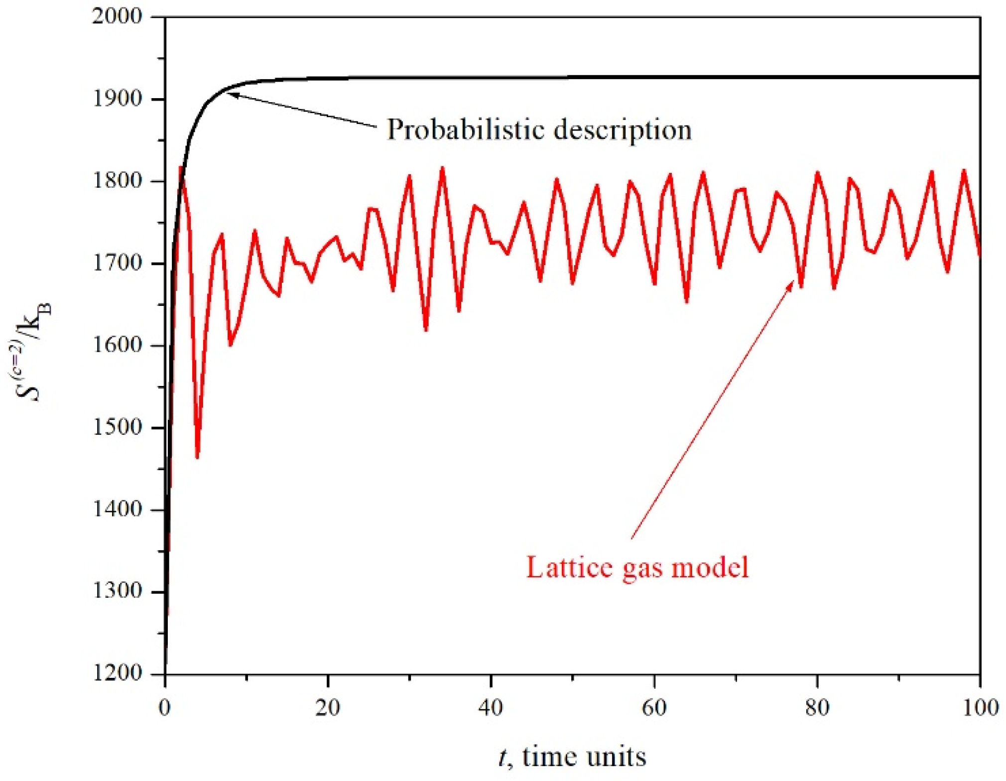
We can now compare the two entropies. The red line of Figure 17 corresponds to the coarse-grained entropy (c = 2) calculated by applying Equation (4) to the evolution of the system with the chessboard-like initial configuration depicted in Figure 13, as the system evolves following the deterministic motion rules of Section 2 (black line of Figure 14). The black line of Figure 17 corresponds to the entropy as calculated using Equation (7); in this case, the predicted evolution of the system follows the probabilistic approach introduced in this section and depicted in Figure 16a–d. Notice that fluctuations are absent, and that the second law of thermodynamics is obeyed:

$$\frac{\mathrm{d}S}{\mathrm{d}t}\ge 0.$$

(8)

The behavior depicted by the black line of Figure 17 is monotonically irreversible.

The transition from time-reversible, deterministic rules of motion (Section 2) to Equation (5), an irreversible kinetic equation, is akin, in spirit, to what Boltzmann achieved in the formulation of the H-theorem, with the introduction of his kinetic equation for the case of dilute gases [1,2,3,4,5,6,7].

7. Beyond the Lattice Gas Model

In the previous section, we discussed how an arrow of time can emerge by introducing probability to the description of the time evolution of a two-dimensional lattice gas. The simplicity of our model prevents us from studying here other types of arrows of time that were proposed. References [21,24] discuss in detail the cosmological, electrodynamic, and radiative arrows of time. In particular, in Penrose’s book [21], we can find an interesting discussion about the roles played by gravitation and the presumably low-entropy initial state of the universe just after the Big Bang regarding the evolution of entropy.

Though the view embraced in this paper is that statistical assumptions are the key ingredients in solving the reversible-to-irreversible transition, it must be mentioned that this is far from being a unique position. As we mentioned in the Introduction, Prigogine is proposed to modify the microscopic fundamental laws of motion in order to obtain intrinsic irreversibility [6,12,13]. In relation to the radiative arrow of time, we mentioned a debate that Walter Ritz and Albert Einstein held in 1909 [25,26]. Ritz argued that radiation asymmetry (which implies irreversibility) in classical electrodynamics is due to an asymmetry in the fundamental laws of electromagnetic radiation, and that it cannot be deduced by purely probabilistic arguments; on the other hand, Einstein maintained that radiative irreversibility can be explained by statistical arguments alone. Interestingly, some authors argued that later on, Einstein himself was not strongly convinced of his own opposition to Ritz’s ideas [26]. Unfortunately, Ritz died shortly after their debate.

It must be mentioned that, under certain assumptions, the Boltzmann kinetic equation can be deduced from the first Bogoliubov–Born–Green–Kirkwood–Yvon (BBGKY) hierarchy equation [2].

Whether the fundamental laws of dynamics are intrinsically irreversible or not, we may ask if the presence of pervasive noise (in the form of photons, phonons, gravitational waves, etc.) will ever allow us to discern between a statistical and a non-statistical origin of irreversibility. Even with new techniques that can probe microscopic systems [27,28,29], it is the opinion of the author that it is too soon to answer such a fascinating question.

8. Summary and Conclusions

We discussed two types of approaches in describing the evolution of the system introduced in Section 2, from an unlikely configuration to a likely one (if the number of particles is very large, we might call the process diffusion or relaxation). In the dynamical approach followed in Section 3, Section 4 and Section 5, all calculations are based on the dynamical laws established in Section 2, though some modifications were required when noise was introduced in Section 5. Coarse graining allowed us to have a description using a smaller number of variables, but the underlying microscopic dynamics remained the same. This must be contrasted to what we carried out in Section 6, where a probabilistic approach was used in order to predict the time evolution of a system.

If in calculating the entropy we make use of the exact state of a system (all particle positions and directions are known), we obtain a constant S = 0 as the system evolves in time, due to the deterministic nature of the rules of motion. On the other hand, when studying the same system from a coarse-grained perspective (c ≥ 1), the entropy S^(c) has a tendency to grow (from unlikely to likely configurations); however, due to fluctuations, instances of dS/dt < 0 happen for short periods of time, contradicting the second law of thermodynamics (of course, the larger the number of particles, the smaller the relative size of the fluctuations; however, fluctuations are always present).

In Section 4, we showed that the introduction of noise destroys the time reversibility of our model. If noise is present, typically, a system evolves toward typical (high entropy) configurations. However, in this case, a fluctuating behavior violates, intermittently, the second law of thermodynamics.

A dynamical approach can result, by chance, in atypical system evolutions (from high to low entropy); however, the average behavior of a large number of events starting from the same initial configuration is expected to be typical. On the other hand, a probabilistic approach (e.g., Boltzmann’s kinetic equation or Equation (5)), results in a monotonically non-decreasing entropy function dS/dt ≥ 0.

We can summarize the arguments presented as follows: If the microscopic dynamical laws of motion are time reversible, noise destroys time reversibility. However, the monotonic irreversibility implicit in the second law of thermodynamics, i.e., dS/dt ≥ 0, is achieved by adopting a probabilistic approach.