Article

Statistical Mechanics of Long Walks in Dynamic Complex Networks: Statistical Arguments for Diversifying Selection †

by
Dimitri Volchenkov
1,* and
C. Steve Suh
2,*
1
Department of Mathematics and Statistics, Texas Tech University, 1108 Memorial Circle, Lubbock, TX 79409, USA
2
Nonlinear Engineering and Control Lab, Department of Mechanical Engineering, Texas A&M University, College Station, TX 77843-3123, USA
*
Authors to whom correspondence should be addressed.
This paper is an extended version of our paper published in the 2022 Conference on Nonlinear Science and Complexity hosted online by the Physics Department of the Aristotle University of Thessaloniki, Thessaloniki, Greece, 26–29 September 2022.
Dynamics 2022, 2(3), 252-269; https://doi.org/10.3390/dynamics2030013
Submission received: 27 June 2022 / Revised: 2 August 2022 / Accepted: 9 August 2022 / Published: 12 August 2022

Abstract

:
We study the thermodynamic limit of very long walks on finite, connected, non-random graphs subject to possible random modifications and transportation capacity noise. As walks might represent the chains of interactions between system units, statistical mechanics of very long walks may be used to quantify the structural properties important for the dynamics of processes defined in networks. Networks open to random structural modifications are characterized by a Fermi–Dirac distribution of node’s fugacity in the framework of grand canonical ensemble of walks. The same distribution appears as the unique stationary solution of a discrete Fokker–Planck equation describing the time evolution of probability distribution of stochastic processes in networks. Nodes of inferior centrality are the most likely candidates for the future structural changes in the network.
PACS:
02.10.Ox; 05.40.Fb; 89.70.+c
MSC:
05Cxx; 05C82; 90Bxx; 91D30

1. Introduction

Dynamic complex networks (DCN) are ubiquitous [1,2]. They are systems whose network properties evolve in time. Defining network behaviors is challenging because the global dynamics of DCNs at the ensemble (macroscopic) level are the manifestation of the coupled constituent dynamics at the individual constituent (microscopic) level [1]. Individual dynamics and global dynamics together define the emergence of collective behaviors such as synchronization and asynchronization at the network level. DCNs dynamics are nonlinear, non-stationary, and complex. Significant efforts have been given to correlate the complex interactions between ensemble constituents with simultaneous collective behaviors as well as critical and abrupt failures when the system is perturbed [3].
Functional units of many real-world systems manifesting themselves as DCNs interact with each other at the different and disparate temporal and spatial scales giving rise to the various behaviors that may not be expressed by a direct sum of individual behaviors of their parts [4]. The networking systems are often metaphorically represented by graphs, in which the graph vertices embody the system functional units, and the graph edges sketch the various interactions between these units. As a knowledge of more detailed characteristics can make a network system appear more complex, its graph representation is essentially observer dependent and therefore not unique [5]. Nevertheless, graph models are useful for the network analysis, as helping us to answer the fundamental question about relations between the local (i.e., pertaining to a single node) and global (of the entire network) properties of a complex system [4].
The first attempt to address this question in the framework of a thermodynamic approach to graphs was initiated in complex network theory (CNT) [6,7]. In the thermodynamic limit of infinitely large graphs  N considered in CNT, any functionally relevant structural features of a graph appear to be asymptotically negligible “fluctuations”; the entire network is viewed as an ever growing collection of structurally homogeneous random graphs; and the famous power law statistics for node’s degree distributions may result from a superposition of the binomial or Poisson degree distributions typical for random graphs [8,9]—true scale-free graphs are rare [10]. The evolution of complex networks is explained in CNT by the preferential attachment mechanism [11] under the spell of Matthew’s principle of accumulated advantage (“For to every one who has will more be given, and he will have abundance; but from him who has not, even what he has will be taken away.” Matthew 25:29, RSV.). Similarly to the formation of a giant component in random graphs [8], a complex network eternally growing in accord with the preferential attachment principle undergoes a topological phase transition from a “rich-get-richer” phase to a “winner-takes-all” phase due to the Bose–Einstein condensation mechanism [6,12,13].
Another thermodynamic approach to the study of complex networks proposed by us recently in [14] concerns the thermodynamic limit of very long walks  n in graphs. On the one hand, infinite walks are possible in finite and even very small graphs, such as those portraying the majority of artificially engineered networking systems and power grids. On the other hand, the statistical ensembles of (random) walks do not require the structure of a backbone graph is random, as it was implicitly assumed in CNT concerning asymptotically infinite graphs. It is obvious that the structures of engineered systems are robust and functionally determined, being anything but random. As the statistics of random walks is essentially sensitive to the graph structural features, such as irregularities, the available cyclic paths, and emerging defects, such as random edge rewiring, dramatically reshaping the global mobility patterns in the entire graph, the proposed thermodynamic approach is also applicable for the analysis of dynamic complex networks (DCN) used to model the evolving relationships between entities. The local fluctuations of path’s growth rate around the graph topological entropy that rise due to the graph structure modifications follow Fermi–Dirac statistics [14].
The major distinguishing features between two approaches are summarized in the following Table 1.
In the present paper, we continue studying the thermodynamic limit of very long walks n in finite connected undirected graphs. In Section 2, we remind the reader three major statistical ensembles of long walks in graphs. In Section 3, we discuss the applications of statistical ensembles for the study of dynamical processes in networks. In Section 4, we generalize the forward Kolmogorov equation for random walks on graphs for the case of “white noise” of strength β > 0 added to edge transportation capacity. The derived Fokker–Planck equation describes the time evolution of probability distributions of stochastic processes defined in networks. In accordance with the unique equation solution, while central hubs accumulate the most of traffic in normally operating transport networks, traffic congestion may catch it at the nodes of low centrality and structural bottlenecks due to the random fluctuations of transportation capacity in networks. In Section 5, we briefly sketch the network evolution theory making use of an analogy with the evolutionary models of stabilizing and diversifying selection. We conclude in the last section.

2. Statistical Ensembles of Walks in Finite Connected Undirected Graphs

The concept of thermodynamic ensembles of long walks has been introduced by us in [14] following the ideas of Gibbs [15]. For example, the microcanonical ensemble (MCE) representing an isolated system with conserved energy corresponds to a collection of walks in a static graph, in which all walks of the same length n are taken with the same probability P n . Isotropic and anisptropic random walks that make up equal probabilities to all available paths of a given length starting at any graph vertex form the canonical ensembles (CNE) of walks. Finally, an open system of walks defined on a graph changing its structure in time due to the growth, withering, or edge rewiring processes that keep the graph topological entropy (GTE) in tact are described by the grand canonical ensemble (GCE), in which every node may be characterized by the quality of being fleeting in the course of network’s transformations—fugacity. In contrast to the classical equilibrium thermodynamics, theses thermodynamic ensembles are not equivalent if defined for walks in graphs, even in the thermodynamic limit n .
In the present section, we discuss these statistical ensembles of walks in details. For simplicity, we shall consider a finite connected undirected graph G ( V , E ) where V, V = N , is a set of graph vertices, and E V × V is a set of edges. We assume that the graph G is defined by an adjacency matrix, A i j = 1 , iff i , j E , but A i j = 0 otherwise, and the adjacency matrix has the following spectral decomposition: A i j = s = 1 N α s u i s u s j , with ordered eigenvalues α max α 1 > α 2 α N where α max is the graph spectral radius (GSR). Since the graph is undirected, its adjacency matrix is symmetric, A i j = A j i , its eigenvalues are real, and the corresponding eigenvectors { u i } i = 1 N form an orthogonal system of vectors in R N .

2.1. The Microcanonical Ensemble of Walks

All walks of length n (n-walks) in MCE are assigned the same probability [14]:
P n exp F n k T ,
in which the (Boltzmann constant and) temperature k T 1 / ln 2 , and the free energy of n–walks F n reads as follows:
F n log 2 P n = k T ln N n = log 2 N n
where N n is the total number of n-walks in the graph G. Using the spectral decomposition of the adjacency matrix, we obtain the following algebraic expression for the free energy of walks [14]:
F n = log 2 N n = log 2 i j A i j n = log 2 i j s = 1 N α s n u i s u j s = log 2 s = 1 N α s n γ s 2 = log 2 γ 1 2 α max n 1 + s = 2 N γ s 2 γ 1 2 α s α max n , γ s i = 1 N u i s .
Since α s / α max < 1 , it follows from (3) that in the limit n the intensive free energy (per edge absorbed by a walk) equals to
μ lim n F n n = lim n 1 n log 2 γ 1 2 α max n 1 + s = 2 N γ s 2 γ 1 2 α s α max n = log 2 α max d G .
log 2 α max in (4) is called the graph topological entropy (GTE) [14,16,17], as being an exponential growth rate of the number of distinguishable n-walks in the graph, a natural measure of complexity in the framework of MCE. The GTE μ can also be interpreted as an effective dimension of space (of the graph), d G . If d -dimensional flat space is modeled by a lattice, or a κ —regular graph (in which every graph vertex has the same number of neighbors, κ = 2 d ), its spectral radius α max = κ , and the GTE equals μ = log 2 κ = d , the dimension of modeled space.

2.2. The Canonical Ensembles of Walks—Random Walks

All n-walks starting at the same vertex i, i V , are taken with equal probability in the CNE [14]. The number of n-walks available from the vertex i, the n-th order degree of the vertex, equals to
κ i n j = 1 N A n i j , κ i 0 = 1 .
Taking into account that κ i n + 1 = j = 1 N A i j κ j n , we obtain the following infinite sequence of irreducible row-stochastic transition matrices defining possible random walks subject to the CNE in G [4,14], viz.,
W i j n = A i j κ j n κ i n + 1 = A i j s = 1 N A n j s s = 1 N A i s s = 1 N A n s r , j = 1 N W i j n = 1 , n N ,
The first order random walk in (6) defined by the transition matrix W i j 1 = A i j / κ i 1 is known for more than a century [18,19,20]. The walk W i j 1 is locally isotropic, as a random walker chooses the next node to visit among all nearest neighbors with equal probability [4,14]. Other random walks defined in (6) by W i j n , n > 1 , make every of κ i n walks available from the node i V with equal probability, and therefore transitions to the nearest neighbors providing more n-walks are more likely to be chosen by the walker than transitions to others, so that these random walks may be locally biased (anisotropic) [4].
In the limit of infinite walks n , the series of transition matrices W i j n converges [4,14] to the Ruelle-Bowen random walk [17], viz.,
W i j = lim n W i j n = lim n A i j κ j n κ i n + 1 = lim n A i j α max n u j 1 γ 1 α max n + 1 u i 1 γ 1 = A i j u j 1 α max u i 1 .
Random walks subject to the CNE are characterized by equilibrium densities (of graph nodes, subgraphs, and currents in the graph) that do not evolve over time, even though the underlying system might be in constant motion. For example, the major left eigenvectors of the row-stochastic transition matrices W i j n , n 1 belonging to the maximal eigenvalue λ = 1 , viz.,
π i n = κ i n κ i n 1 s = 1 N κ s n κ s n 1 , s = 1 N π r n W r s n = π s n
constitute the stationary distributions of random walks defined by W i j n on the graph G.
The first—order stationary distribution π i 1 = κ i 1 / 2 | E | , where | E | is the total number of edges in the graph G, informs us about the normalized number of links incident upon a node—its degree centrality. The stationary distribution for the Ruelle-Bowen random walks, π i = u i 1 2 [21] is related to the eigenvector centrality  u i 1 of the node i in the graph G [22].
The GTE (playing the role of an effective dimension of space for the walks subject to the MCE, see Section 2.1) turns into a direction-dependent graph space dimension tensor in the context of CNE random walks (6) and (7), viz.,
Δ i j ( n ) log 2 κ i ( n ) κ j ( n 1 ) , Δ i j ( ) = log 2 α max u i 1 u j 1 ,
measuring the degree of directional anisotropy of random transitions in CNE [14].

2.3. Grand Canonical Ensemble of Walks

Systems exchanging energy and particles with a heat bath in thermodynamic equilibrium are described by the GCE [15]. The GCE statistics can be applied to the study of the DCN, acquiring or losing nodes in the course of interaction with the environment, or other networks. Although the global growth rate of the number of distinguishable walks possible in a graph tends to the GTE, μ = log 2 α max , in the thermodynamic limit n , the local growth rate of the number of distinguishable walks available from a node, log 2 α max γ 1 u i 1 , may be inferior to the GTE. The GTE μ plays the role of a chemical potential considered fixed for the entire DCN being in a “thermodynamic equilibrium” with the environment in GCE.
In the framework of GCE, the probability to observe such a local “fluctuation” of the intensive free energy at the node i V (due to the local n-walks growth rate inferior to the GTE μ ) for the very long walks n is taken to be [14]:
P i ( n ) = 1 Z n exp n μ log 2 α max n u i 1 γ 1 k T ,
in which k T 1 / ln 2 and Z n is the grand partition function, playing the role of a normalization factor in (10). In the thermodynamic limit of infinite walks n , the exponential factor in (10) representing node’s fugacity in the DCN takes the following form:
lim n exp n μ log 2 α max n u i 1 γ 1 k T = lim n exp [ log 2 α max n log 2 α max n u i 1 γ 1 ] 1 / ln 2 = 1 u i 1 γ 1 , γ 1 j = 1 N u j 1 ,
so that the grand partition function Z that amasses fugacity over all nodes in the graph G reads as follows:
Z lim n Z n = 1 γ 1 j = 1 N 1 u j 1 , γ 1 i = 1 N u i 1 .
Finally, taking into account (11) and (12), we obtain the limiting probability quantifying the ease of separation/amendment of a vertex from/to the network at the node i w.r.t. the system of infinitely long walks n as
P i = lim n P i ( n ) = u i 1 1 j = 1 N u j 1 1 = 1 1 + u i 1 j i N u j 1 1 1 1 + exp ε i M k T
that takes the form of a Fermi–Dirac distribution of fermions in a single-particle state i of the energy ε i log 2 u i 1 j i N u j 1 1 , with zero chemical potential M = 0 of adding/removing a new node if it does not change the system of walks in the graph, and temperature k T 1 / ln 2 . In the thermodynamic limit of infinite walks, any change to the (free) energy is associated to a modification of the system of possible walks in the graph while a node can leave and enter the graph at no cost. The local increment of free energy due to the disappearance of node from the graph is known as entropic pressure discussed by us in [14].
The distribution (13) of relative fugacity of vertices from/into the network can be considered as a normalized inverse eigenvector centrality. The graph vertices with the inferior growth rate of infinitely long walks that they host appear to be insufficiently integrated into the graph structure, and therefore they might be lost, or, on the contrary, acquire new connections in the course of graph structural modifications. The grand canonical potential, viz.,
Ω = k T ln Z = log 2 1 γ 1 j = 1 N 1 u j 1 ,
plays the role of free energy with respect to the grand partition function Z in GCE, and k T 1 / ln 2 .
The Fermi–Dirac distribution, previously observed only in a quantum system of non-interacting fermions, appears in the model due to the non-interacting quality of walks in the graph, similar to the Pauli exclusion principle allowing for only two possible microstates for each single-particle level.

3. Applications of Statistical Mechanics of Walks

In the present section, we discuss some applications of the statistical ensembles of walks for the analysis of feedback loops, determinantal processes, structurality, controllability, and predicatability of walks in graphs.

3.1. Backbones for Feedback: Expected Numbers of Cyclic Walks per Graph’s Size

Positive and negative feedback loops are at the core of self-regulating and controlling mechanisms, regenerative circuits, amplifiers, and other complex dynamical systems in engineering, economics, and biology [23]. The graph cyclic structures serve as a base for the feedback arc sets of cause and effect that form a circuit or loop [24]. The expected numbers of cyclic walks of the given periods that can be activated in a graph of a given size and structure is an important characteristic of the feedback arc sets. The expected numbers of cyclic walks per graph size can be found by applying the Cayley–Hamilton theorem [25] (stating that every square matrix over a commutative ring satisfies its own characteristic equation) to the random walk transition matrices W i j n defined for some n 1 in Section 2.2. The characteristic polynomial det ( t I W ) = 0 of a N × N transition matrix W is monic (its leading coefficient is 1), and therefore an analogous polynomial in a transition matrix W can be interpreted as a regression relation for the probability to reach the graph vertex j starting from the graph vertex i precisely in N steps (i.e., for the N-th degree of transition matrix W), viz.,
W i , j N = k = 1 N ( 1 ) k + 1 Tr k W W N k i , j .
The regression relation (15) shows that the probability for a random walker to get from i to j precisely in N steps is an expectation value over the probabilities to reach j from i in shorter times: N 1 , N 2 , , 0 , weighted by Tr k W , the expected numbers of cyclic walks of the period k possible for a random walker per N steps in the given graph. The trace of the k-th exterior power of W is the k-th coefficient of the characteristic polynomial of the matrix W and can be calculated as a single determinant, viz.,
Tr k W = 1 k ! Tr W k 1 0 Tr W 2 Tr W k 2 Tr W k 1 Tr W k 2 1 Tr W k Tr W k 1 Tr W .
The expected numbers of cycle walks of the period k per N steps (16) are the algebraic invariants of all transition matrices W ( n ) , for any random walk order n 1 , as being related to the graph topological properties (i.e., the numbers of k-loops that can be made in N steps).
The characteristic polynomial coefficients for a transition matrix defined on the graph can be efficiently calculated using the recursive Faddeev–Le Verrier algorithm [26]. In Figure 1, we have shown the spectrum of the expected numbers of cycle walks (or a partition of a N-walk into the cycles of different lengths) a walker can perform in the Flower snark graph (left panel) and in the Kittel graph (right panel), respectively. The presented above diagrams show the possibility of co-existence and co-functioning of the feedback loops of different periods in DCN.

3.2. Determinantal Processes Induced by Canonical Ensembles

Walks subject to CNE are characterized by the equilibrium densities over individual vertices, subgraphs, and random currents in a finite connected undirected graph. These densities can be calculated as the squared determinants of minors made up from the eigenvectors of the symmetrized transition matrices. The corresponding stochastic point processes are called determinantal process, or fermionic processes [27] motivated by the use of Slater determinants in quantum mechanics [28], with multiple applications in physics [29], wireless network modeling [30,31], and in random matrix statistics [32].
By performing a similarity transformation, we make the transition matrix W i j ( n ) to a symmetric form [4,33], viz.,
W ^ i j ( n ) = A i j κ j ( n ) κ i ( n ) κ j ( n + 1 ) κ i ( n + 1 )
The similarity transformation does not change the matrix spectrum. In the what following, we denote the symmetric transition matrix W ^ , omitting the random walk order index n for keeping the notations simple. The symmetric transition matrix (17) can be written in a spectral form:
W ^ = Ψ Λ Ψ , Ψ = Ψ 1 O ( N ) , det Ψ Sgn ( Ψ ) = ± 1 ,
in which Λ is a diagonal matrix of eigenvalues with real valued entries 1 = λ 1 > λ 2 λ N 1 . Each eigenvalue λ k , k = 2 , N , corresponds to an eigenmode (a random current) characterized by the relaxation time toward a stationary distribution τ k = 1 / ln ( 1 λ k ) . The maximal eigenvalue λ 1 = 1 (of multiplicity 1) corresponds to a graph stationary process. The columns ψ k : V S 1 N 1 and rows ψ k : V S 1 N 1 of the orthogonal matrix Ψ form the orthonormal bases in R N . The k-th order wedge products, ψ i 1 ψ i k and ψ i 1 ψ i k , are the determinants of the corresponding k-th order minors of Ψ in (18). The space of exterior forms k R N , k = 0 , N ( 0 R N = R , 1 R N = R N ) has the dimension N k . The properties of determinants of minors of matrices composed of orthonormal vectors were discussed in [34] in detail. These wedge products form the orthonormal basis of the space k R N , viz.,
ψ i 1 ψ i k , ψ j 1 ψ j k = δ i 1 , j 1 δ i k , j k , ψ i 1 ψ i k , ψ j 1 ψ j k = δ i 1 , j 1 δ i k , j k ,
so that the squared determinants of the k-th order minors of the orthogonal matrix Ψ define the properly normalized probability distributions over the index set { i 1 , , i k } :
ψ i 1 ψ i k 2 = 1 , ψ i 1 ψ i k 2 = 1 .
An elementary example of this property is given by the Perron (major) eigenvector of a symmetric transition matrix, ψ 1 (whose elements can be considered as the primitive minors of order 1). Indeed, the squared elements of ψ 1 determine a stationary distribution of random walks over the individual graph nodes, ψ 1 , i 2 = π i , i V π i = 1 .
To show the compatible stationary distributions over the higher-order minors, we consider random walks in a triangle graph (Figure 2).
All random walks transition probabilities between vertices of a triangle equal to 1 / 2 (for any order of random walks). The orthonormal eigenvectors of the symmetric transition probability matrix are given in the rows of Table 2. It is easy to check that the top eigenvector belonging to λ = 1 defines the equal density for every vertex, ( 0.57735 ) 2 = 1 / 3 , as expected.
The following squared determinants of the 2-nd order minors ( all summing to 1) define the stationary distributions over the pairs of indices (all compatible with the equitable density of random walkers over triangle’s vertices):
ψ 1 ψ 2 2 = 0.57735 0.57735 0.44988 0.81503 2 + 0.57735 0.57735 0.44988 0.36515 2 + 0.57735 0.57735 0.81503 0.36515 2 = 0.53333 + 0.00239 + 0.46427 = 1 ;
ψ 1 ψ 3 2 = 0.57735 0.57735 0.68138 0.04892 2 + 0.57735 0.57735 0.68138 0.73030 2 + 0.57735 0.57735 0.04892 0.73030 2 = 0.13333 + 0.66427 + 0.20239 = 1 ;
ψ 2 ψ 3 2 = 0.44988 0.81503 0.68138 0.04892 2 + 0.44988 0.36515 0.68138 0.73030 2 + 0.81503 0.36515 0.04892 0.73030 2 = 0.33333 + 0.33333 + 0.33333 = 1 ;
ψ 1 ψ 2 2 = 0.57735 0.57735 0.44988 0.81503 2 + 0.57735 0.57735 0.68138 0.04892 2 + 0.44988 0.81503 0.68138 0.04892 2 = 0.53333 + 0.13333 + 0.33333 = 1 ;
ψ 1 ψ 3 2 = 0.57735 0.57735 0.44988 0.36515 2 + 0.57735 0.57735 0.68138 0.73030 2 + 0.44988 0.36515 0.68138 0.73030 2 = 0.00239 + 0.66427 + 0.33333 = 1 ;
ψ 2 ψ 3 2 = 0.57735 0.57735 0.81503 0.36515 2 + 0.57735 0.57735 0.04892 0.73030 2 + 0.81503 0.36515 0.04892 0.73030 2 = 0.46427 + 0.20239 + 0.33333 = 1 ;
In the diagrams presented in Figure 3, we highlighted the pairs of indices (the connecting edges in triangles) by color and width in accordance with the probabilities (the values of individual squared determinants) in (21)–(26). The diagrams show stationary configurations admissible in a triangle structure, and the equitable configuration (of 1 / 3 s) is only one of them. Each diagram in Figure 3a can be characterized by the Shannon entropy, S = i , j P i , j log 2 P i , j , i , j = 1 , 2 , 3 , reflecting the diversity of probabilities P i , j in the admissible stationary densities over the pair of indices. The obtained entropy values range from 1.585 bits (for the equitable configuration) to 0.941 bits for the most unequal partition. All six entropies are made up into a matrixplot shown in the right panel of Figure 3b helping to visualize the diversity of stationary configurations possible on the graph.
We conclude this subsection with a remark on that a triangle is a very simple graph, as the corresponding transition matrix in all order of the random walks n is the same. In the more complex and uneven structures, the behavior of random walks for the different orders n > 1 vary dramatically due to the increasing degree of anisotropy and the decreasing mixing time (growing spectral gap) of walks [14].

3.3. Information Flows Associated with Canonical Ensembles

Information is the resolution of uncertainty about the admissible patterns of future behavior [35]. To discuss information in a system, we need to define a canonical ensemble of states of the system first [14]. In the context of walks in graphs, information comes from lumping of many particular long walks (microstates) into a single macrostate characterized by some stationary distribution for the individual vertices ( π ), subgraphs, and random currents as discussed in Section 3.2.
If n r counts the number of visits paid by a walker to the r-th vertex in the course of such a walk of length n = r n r that n r / n π r , r π r = 1 as n , all these walks are lumped into a single π -macrostate. The total number of lumped walks is given by the multinomial coefficient, viz.,
n ! n π 1 ! n π N ! exp n H , H r π r ln π r ,
as n [14]. Therefore, the Boltzmann-Gibbs-Shannon entropy H [36,37] in (27) appears as a growth rate of the multinomial coefficient as n . The free energy over the canonical ensemble of such very long n-walks subject to CNE is F n k T · n H , and the intensive free energy of walks per absorbed edge (4) equals to
μ = lim n F n n = r π r log 2 π r H ( X t ) ,
i.e., the expected amount of information released at each step t of the π -walk { X t V : t Z } , in which Pr ( X t = r ) = π r [14].
  • Structurality of a Graph w.r.t to a Random Walk:
On the one hand, our ability to predict the future walk in a graph can be assessed by the conditional entropies H X t | X t 1 , X 1 , t 1 that quantify the amount of information released when the present vertex of the walk X t becomes known given the previous history. For a walk defined by a transition matrix W i j , the information calculations are feasible [4,14,38,39], as evolution of a Markov process in the future depends only on the present state and does not depend on past history [40]. Indeed, the time average of the conditional entropy of the present conditioned on the past for Markov chains reads as follows:
lim T 1 T t = 1 T H X t | X t 1 , X 1 = lim T 1 T H ( X 1 ) + H X 2 | X 1 + H X 3 | X 2 + = lim T 1 T H ( X 1 ) + T 1 T H X 2 | X 1 = H X 2 | X 1 H X t + 1 | X t = k = 1 N π k s = 1 N W k s log 2 W k s .
The entropy excess [41,42,43] over the entropy rate (29), viz.,
S = H X t H X t + 1 | X t , = k = 1 N π k log 2 π k + s = 1 N W k s log 2 W k s = k = 1 N π k log 2 π k s = 1 N W k s W k s ,
characterizes the amount of uncertainty about the future step that can be resolved from past history of the walk predetermined by the graph structure, [4,14,38,39]. In the present paper, we call this information component “structurality” (measured in bits) having in mind the quality of structure the graph possesses w.r.t a random walk defined by the transition matrix W i j .
  • Controllability of a Random Walk defined in a Graph:
On the other hand, our ability to control the future step of a walk defined in a graph can be assessed by the conditional mutual information  I X t + 1 , X t | X t 1 between the present and the future vertices visited by the walk conditioned on past history [14], viz.,
C = H X t + 1 | X t 1 H X t | X t 1 = k = 1 N π k r = 1 N W k r log 2 W k r W k r 2 log 2 W k r 2 = k = 1 N π k log 2 r = 1 N W k r W k r ( W k r 2 ) W k r 2 .
We call this information component “controllability” having in mind that it quantifies the consequence of presence at a vertex for reaching another vertex at the next step of the walk w.r.t to a random walk defined by the transition matrix W i j .
Both information components, S and C , taken together gauge the amount of apparent uncertainty about the future walker’s location in the graph that can be resolved by observing past history and applying some graph navigation strategy compatible with the chosen CNE. Summing up these components together, we call this part of information predictable [4,14,38,39].
  • Ephemerality of Random Walks defined in a Graph:
The following formal calculation involving entropy and the aforementioned conditional entropies shows the remaining part of information, neither relevant to the past, nor to the future [14]. First, we add and subtract the conditional entropies from H ( X t ) and then isolate the structurality ( S ) and colntrollability ( C ) information components forming the predictable part of information ( P ):
H X t = H ( X t ) H X t + 1 | X t S + H X t + 1 X t 1 H X t X t 1 C P + H X t + 1 X t + H X t X t 1 H X t + 1 X t 1 U .
The remaining combination of conditional entropies denoted in (32) by U (for “unpredictable”), obviously, represents the amount of true uncertainty anchored at the present state of the walker only that cannot be inferred anyway [14]. Following [43], this information component can be called “ephemeral”, and the corresponding quality of random walks on the graph—ephemerality.
The decomposition of entropy for the random walks of different orders defined on a graph can be conveniently visualized with the use of radar graphs as shown in Figure 4.
Two triangles (one shown by a bold line, and a dashed line used for another) presented on the radar graphs in Figure 4 depict the information decomposition H = S + C + U for the two orders of random walks. Namely, the bold line triangle displays three information components associated to the isotropic nearest neighbor random walk defined by the transition matrix W i j ( 1 ) . The dashed triangles show the partition of entropy associated to the anisotropic walk defined by the matrix W i j ( ) taking all infinite walks starting from a node with equal probabilities. Random walks on both graphs (shown in the left right panels of Figure 4) are characterized by the high degree of predictability.
Using the Markov chain models of musical compositions based on the standard MIDI representation of music projected to a single octave ( 12 × 12 matrices), we can study the partition of entropy in musical pieces [4,44,45] in the same way, as we did with graphs. Two examples of such a partition are shown in Figure 5.
The information flow associated to the first order random walks defined on the musical networks of European tonal music is dominated by the controllability components (determining the influence of a present state of the Markov chain, a musical note, on the forthcoming state). The related bold lines triangles shown in Figure 5 are skewed toward controllability corner of the radar plots. In contrast to them, the random walks of infinite order mostly account for the large scale structures in a musical composition that are always in tune with the particular tonality scale, musical style and the human feeling of musical harmony [4].
The possible applications of entropy decomposition to the predictability analysis of stock price dynamics based on the five years of the daily Standard & Poor’s data were discussed in [46]. In [14], the entropy decomposition was considered in a context of navigation through graphs and urban environments.

4. Fugacity Distribution as a Stationary Solution of a Discrete Fokker–Planck Equation

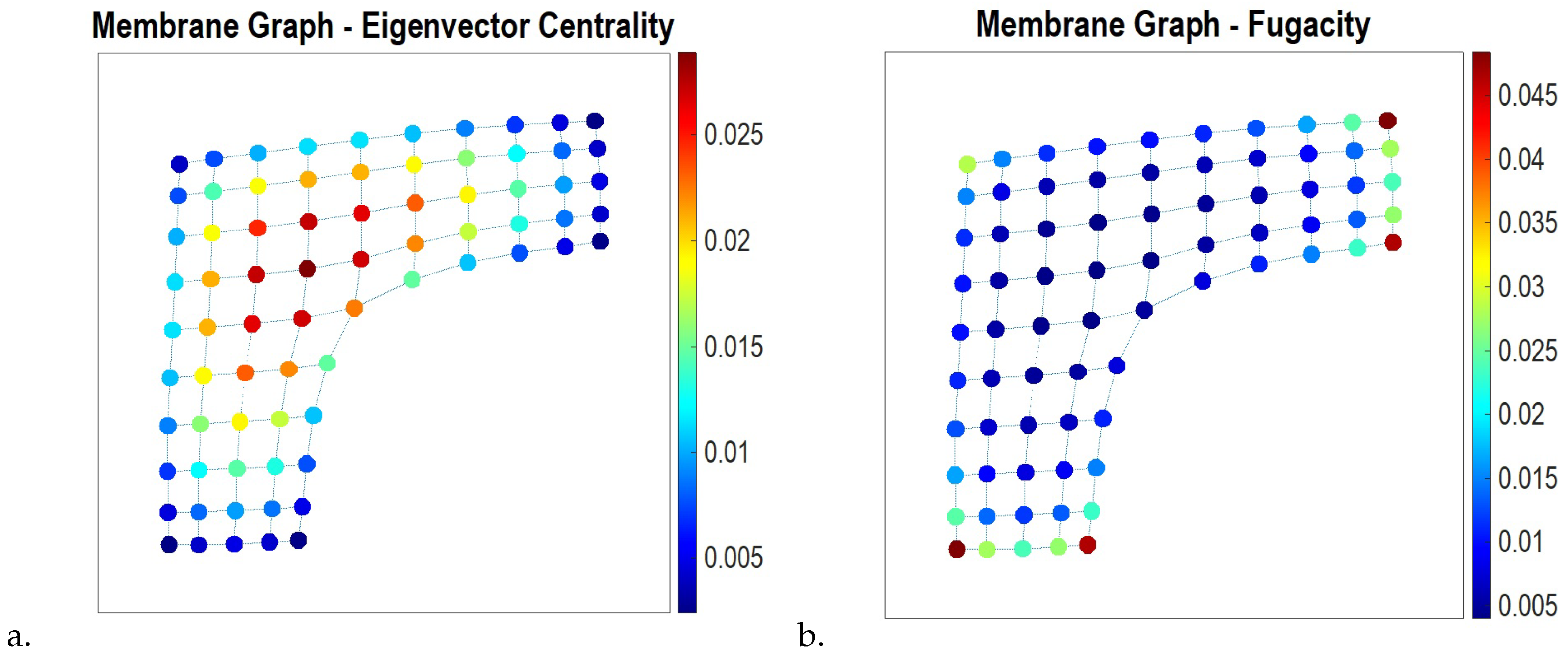
The GCE is used to describe open systems exchanging energy and particles with the environment in a state of thermodynamic equilibrium (Section 2.3). In the context of infinitely long walks in graphs, graph vertices are characterized by their ease of removing from the graph—fugacity, a relative inverse eigenvector centrality of the vertex. The less important the vertices w.r.t. very long walks, the higher chance the network structure will be modified at them by wiring new connections to better integrated nodes and subgraphs, or by their removal from the network. In Figure 6, we have contrasted the structurally opposite location of vertices of high centrality and high fugacity in a membrane graph. The vertices that are prone to possible modifications, as being of minimal centrality, are located right at the corners of the membrane.
Interestingly, a Fermi–Dirac distribution involving (noise dependent) fugacity also appears as the unique stationary solution of a Fokker–Planck equation describing the continuous -time dynamics of distributions subject to the CNE under “noisy” transportation capacity and random edge rewiring in a graph. For keeping the what following calculations simple, let us consider the limiting transition operator of the Ruelle-Bowen random walk (7) in a finite connected undirected graph G ( V , E ) defined by an adjacency matrix A i , j , viz.,
W i j ( ) = A i j α m a x exp log 2 u j 1 log 2 u i 1 = A i j exp log 2 u j 1 log 2 u i 1 μ A i j exp Q i j
where u 1 is the Perron eigenvector belonging to the maximal eigenvalue α max of the adjacency matrix A i j , log 2 u i 1 is a discrete potential function of the Ruelle-Bowen random walk (7), μ = log 2 α max is the GTE (4) playing the role of a chemical potential of very long walks in the graph, and Q i j is its generating matrix. The potential functions of Markov processes defined on graphs and their relations to the Fokker–Planck equations have been discussed in [47,48]. The continuous time evolution of a probability distribution ρ i ( t ) = Pr X ( t ) = i , i V is then described by a forward Kolmogorov equation [49], viz.,
ρ ˙ i ( t ) = j V ρ j ( t ) Q i , j = j V , u j 1 < u i 1 ρ j ( t ) log 2 u j 1 log 2 u i 1 μ + j V , u j 1 > u i 1 ρ i ( t ) log 2 u j 1 log 2 u i 1 μ
supplied with some initial condition ρ ( 0 ) . As was observed in [47], the Fokker–Planck equation can be obtained by adding “white noise” described by the Wiener process, d X t = Q X t d t + 2 β d W t , with strength 2 β to the Kolmogorov Equation (34). The Fokker–Planck equation keeps the form of (34) although written down for the Onsager potential [50]: log 2 u i 1 log 2 u i 1 + β log 2 ρ i ( t ) = log 2 u i 1 ρ i β ( t ) , i V , viz.,
ρ ˙ i ( t ) = j V , u j 1 ρ j β ( t ) < u i 1 ρ i β ( t ) ρ j ( t ) log 2 u j 1 ρ j β ( t ) log 2 u i 1 ρ i β ( t ) μ + j V , u j 1 ρ j β ( t ) > u i 1 ρ i β ( t ) ρ i ( t ) log 2 u j 1 ρ j β ( t ) log 2 u i 1 ρ i β ( t ) μ .
The Fokker–Planck Equation (35) describes the time evolution of a modified, time inhomogeneous Ruelle-Bowen random walk perturbed by “white noise” of the strength 2 β of transport capacity, viz.,
W ˜ i , j ( β , ) ( t ) = A i j α max u j 1 u i 1 ρ j ( t ) ρ i ( t ) β .
In the absence of noise, β = 0 , the Fokker–Planck Equation (35) turns back into the Kolmogorov Equation (34), and the perturbed transition operator (36) takes again the form of the Ruelle–Bowen transition operator (7). The distribution ρ i ( t ) then rapidly converges for any initial condition ρ ( 0 ) to a stationary distribution of the Ruelle–Bowen walk featured by the squared eigenvector centrality of vertices in the graph.
For all β > 0 , it can be shown by a direct computation that the unique, noise dependent stationary distribution satisfying the Fokker–Planck Equation (35) is the Gibbs distribution, viz.,
ρ i * ( β ) = 1 Z exp μ log 2 u i 1 β k T = 1 Z 1 u i 1 1 / β , Z i V u i 1 1 / β
that takes the form of a Fermi–Dirac distribution,
ρ i * ( β ) = 1 1 + u i 1 1 / β j i u j 1 1 / β ,
coinciding with the relative fugacity distribution derinved for the GCE (13) in the particular case of β = 1 . Finally, in the case of very strong noise, β = , the stationary solution (38) converges to a uniform distribution over graph’s nodes independently of the graph structure, viz.,
ρ i * ( ) = lim β 1 1 + u i 1 1 / β j i u j 1 1 / β = 1 N .

5. Discussion: Statistical Grounds for Diversifying Selection

Since DCNs are ubiquitous in the real world, including complex biological and ecological systems, their evolution might be described in terms of the theory of evolution in reference to the process of natural selection. In the present section, we would like to discuss a possible connection between statistics of walks emerging in two thermodynamic limits, the limit of infinite graph N and the limit of infinite walks n , and the modes of natural selection. Specifically, we are interested in two types of natural selection, which have the intrinsic characteristic time scales and, therefore, might be observed in finite time.
Stabilizing selection, in which the population mean stabilizes on a particular non-extreme trait during some characteristic time of stabilization [51], favors the most common phenotype in the population [52]. In the theory of stabilizing selection [53], the principle of accumulated advantage and positive feedback resulting in the reproductive success of the average phenotypes are considered as the major mechanisms limiting the individual variability. Obviously, the CNT that explains the growth of complex evolving networks in the spirit of preferential attachment makes use of an analogy with evolutionary models of stabilizing selection. By assigning an intrinsic fitness value to each node—the higher the fitness, the higher the probability of attracting new edges [54]—an operator initiates the Bose–Einstein condensation mechanism driving a phase transition of the network topology to the appearance of a few “super hubs” of the maximal centrality and of the highest fitness accumulating all branches of the network as N [12,13].
Such a theory certainly was not complete, since it did not explain another important type of natural selection—diversifying, or disruptive selection describing changes in population genetics favorable to the extreme values for a trait over the normative values formed by in the course of stabilizing selection process [52]. Disruptive selection occurs in times of rapid environmental change, such as habitat change or change in resources availability [55,56]. The characteristic time of speciation through a phyletic gradualism mode of evolution enough for the variance of the trait to increase and for the population to be divided into two (or more) distinct groups defines an intrinsic time scale of the diversifying selection process [57,58]. Our work provides the statistical ground for “diversifying selection” in DCN, in the thermodynamic limit of infinite walks n . We have shown that if the DCN is open to random structural modifications, or if the transportation capacity is affected by “white noise”, centrality flips its role in the network dynamics. Namely, the nodes of minimal centrality loosely integrated into the fabric of the network would most likely feature its structural modifications. Concentration of walkers in a “noisy” transportation network (traffic congestion) would most likely to occur at the nodes of lowest centrality and in structural bottlenecks (see Figure 7, right panel). In Figure 7, we have shown the Minnesota Road Network with its vertices highlighted accordingly their eigenvector centrality (left panel) and their fugacity (right panel).
We are very grateful to our reviewer for a profound and interesting question about the possibility of using the preferential attachment principle as a specific algorithm for network evolution corresponding to diversifying selection. On the one hand, as we wrote in the Introduction section, the preferential attachment mechanism referred to the Matthew effect of accumulated advantage determines network’s evolution as the eternal growth by adding nodes subjected to the Bose—Einstein statistics and concluding at the Bose–Einstein condensation in complex networks, in which the fittest “winner” takes all of the evolving graph. In contrast to it, the Fermi–Dirac statistics originally describing identical particles that obey the Pauli exclusion principle does not allow for condensation (of particles at a single state). The thermodynamics limit of infinite walks subjected to the Fermi–Dirac statistics neither requires a network to grow, nor predicts any “eventual stage” of its structural evolution. Similarly, while stabilizing selection fosters a final “condensate” (stabilization) of the entire population on a single trait, or the most common phenotype, disruptive selection favors the speciation in the population in times of rapid environmental changes. On the other hand, abandoning the principle of accumulated advantage, we can propose a recurrent stochastic algorithm for the gradual improvement of a network’s structure based on the fugacity distribution. Namely, new edges may be sequentially added to the network in a random or partly random fashion preferably connecting to the most “disadvantageous” nodes characterized by the maximal fugacity value. The new connection increases the fraction of very long walks hosted by such a node, improving nodes’ connectivity and reducing its fugacity. The change of (free) energy due to amendment/removal of an edge and the related change in the network mobility patterns may be described by entropic forces as discussed in [14]. Then, the fugacity scores are re-calculated for all nodes of the modified graph, and a new edge is added randomly with a preference given accordingly to the renewed fugacity distribution. In such an algorithm, high fugacity attracts the future structural modification, precisely as assumed in the framework of the GCE of walks (Section 2.3). As it is seen in Figure 7b, the nodes of prominent fugacity in the real-world transportation network appear to cluster together, as being located physically proximate to each other and forming ghettos of vertices poorly integrated into the network. The phenomenon of structural clustering of relatively isolated suburbs was discussed in [59,60]. The physical proximity of nodes with high fugacity calling for the urgent structural improvements makes applications of the proposed algorithm to the real-world transportation networks economically feasible, as requiring only the local structural modifications of the underlying graph.

6. Conclusions

In the present paper, we study the statistical ensembles of very long walks defined in finite connected graphs. We developed three important applications of these statistical ensembles to the analysis of network dynamics concerning the feedback and determinantal processes in DCN, as well as the properties of information flows in networks associated with the structurality, controllability, and predictability of walks in the network. The special attention in our work has been given to the DCN open to random structural modifications described in the framework of GCE of very long walks. Fugacity of a node quantifies the likelihood of local structural modifications at the node in the course of network evolution.
For describing the time evolution of probability distributions of stochastic processes defined on graphs, we introduced a discrete finite version of the Fokker–Planck equation as a generalization of the Kolmogorov equation for the different values of “white noise” strength β > 0 affecting transportation capacity in the network. Being the unique stationary solution of the derived Fokker–Planck equation, the Gibbs distribution takes the form of a Fermi–Dirac distribution, coinciding with the relative fugacity distribution of GCE of walks for β = 1 . In the case of very strong noise, the stationary solution of the Fokker–Planck equation converges to a uniform distribution over graph’s nodes, independently of the network structure.
Our work contributes to the evolution theory of DCN by providing a statistical ground for the “diversifying selection” mechanism featuring the loosely integrated nodes as the most likely place for the future network developments fostered by random structural changes in the network.

Author Contributions

Conceptualization, D.V. and C.S.S.; methodology, D.V.; software, D.V.; validation, D.V. and C.S.S.; formal analysis, D.V. and C.S.S.; investigation, D.V. and C.S.S.; resources, D.V. and C.S.S.; writing—original draft preparation, D.V.; writing—review and editing, C.S.S.; visualization, D.V. All authors have read and agreed to the published version of the manuscript.

Funding

This research received no external funding.

Institutional Review Board Statement

Not applicable.

Informed Consent Statement

Not applicable.

Data Availability Statement

The data are contained within the article.

Acknowledgments

The authors are grateful to their universities for the administrative and technical support.

Conflicts of Interest

The authors declare no conflict of interest.

Abbreviations

The following abbreviations are used in this manuscript:
CNTcomplex network theory
DCNdynamic complex networks
MCEmicrocanonical ensemble (of walks)
CNEcanonical ensemble (of walks)
GCEgrand canonical ensemble (of walks)
GSRgraph spectral radius
GTEgraph topological entropy

References

  1. Yang, C.-L.; Suh, C.S. A General Framework for Dynamic Complex Networks. J. Vib. Test. Syst. Dyn. 2021, 5, 87–111. [Google Scholar] [CrossRef]
  2. Shettigar, N.; Yang, C.-L.; Tu, K.-C.; Suh, C.S. On The Biophysical Complexity of Brain Dynamics: An Outlook. Dynamics 2022, 2, 114–148. [Google Scholar] [CrossRef]
  3. Yang, C.-L.; Suh, C.S. On Controlling Dynamic Complex Networks. Phys. Nonlinear Phenom. 2022; Undergoing 2nd review. [Google Scholar]
  4. Volchenkov, D. Grammar of Complexity: From Mathematics to a Sustainable World. In Nonlinear Physical Science; World Scientific Series; Higher Education Press: Beijing, China, 2018; pp. 1–3. [Google Scholar]
  5. Johnson, J. Hypernetworks in the Science of Complex Systems. In Complexity Science; World Scientific Series; Imperial College Press: London, UK, 2014; Volume 3. [Google Scholar]
  6. Albert, R.; Barabási, A.-L. Statistical mechanics of complex networks. Rev. Mod. Phys. 2002, 74, 47–49. [Google Scholar] [CrossRef]
  7. Newman, M. Networks: An Introduction; Oxford University Press: Oxford, UK, 2010. [Google Scholar]
  8. Bollobás, B. Random Graphs, 2nd ed.; Cambridge University Press: Cambridge, UK, 2001. [Google Scholar]
  9. Frieze, A.; Karonski, M. Introduction to Random Graphs; Cambridge University Press: Cambridge, UK, 2015. [Google Scholar]
  10. Broido, A.D.; Clauset, A. Scale-free networks are rare. Nat. Commun. 2019, 10, 1017. [Google Scholar] [CrossRef] [PubMed]
  11. Barabási, A.-L.; Albert, R. Emergence of scaling in random networks. Science 1999, 286, 509–512. [Google Scholar] [CrossRef] [PubMed]
  12. Bianconi, G.; Barabási, A.-L. Bose–Einstein condensation in complex networks. Phys. Rev. Lett. 2001, 86, 5632–5635. [Google Scholar] [CrossRef] [PubMed]
  13. Bianconi, G.; Barabási, A.-L. Competition and multiscaling in evolving networks. Europhys. Lett. 2001, 54, 436–442. [Google Scholar] [CrossRef]
  14. Volchenkov, D. Infinite Ergodic Walks in Finite Connected Undirected Graphs. Entropy 2021, 23, 205. [Google Scholar] [CrossRef]
  15. Gibbs, J.W. Elementary Principles in Statistical Mechanics; Charles Scribner’s Sons: New York, NY, USA, 1902. [Google Scholar]
  16. Adler, R.L.; Konheim, A.G.; McAndrew, M.H. Topological entropy. Trans. Am. Math. Soc. 1965, 114, 309–319. [Google Scholar] [CrossRef]
  17. Delvenne, J.C.; Libert, A.S. Centrality measures and thermodynamic formalism for complex networks. Phys. Rev. E 2011, 83, 046117. [Google Scholar] [CrossRef] [PubMed]
  18. Pearson, K. The Problem of the Random Walk. Nature 1905, 72, 294. [Google Scholar] [CrossRef]
  19. Lovász, L. Random Walks on Graphs: A Survey. In Combinatorics, Paul Erdös is Eighty; Bolyai Society, Mathematical Studies: Keszthely, Hungary, 1993; Volume 2, pp. 1–46. [Google Scholar]
  20. Aldous, D.; Fill, J.A. Reversible Markov Chains and Random Walks on Graphs; Unfinished Monograph, Recompiled 2014; 2002. Available online: http://www.stat.berkeley.edu/~aldous/RWG/book.html (accessed on 27 June 2022).
  21. Burda, Z.; Duda, J.; Luck, J.M.; Waclaw, B. Localization of the Maximal Entropy Random Walk. Phys. Rev. Lett. 2009, 102, 160602. [Google Scholar] [CrossRef]
  22. Landau, E. Zur relativen Wertbemessung der Turnierresultate. Deutsches Wochenschach 1895, 11, 366–369. [Google Scholar]
  23. Åström, K.J.; Murray, R.M. Feedback Systems: An Introduction for Scientists and Engineers; Princeton University Press: Princeton, NJ, USA, 2008. [Google Scholar]
  24. Ford, A. Chapter 9: Information feedback and causal loop diagrams. In Modeling the Environment; Island Press: Washington, DC, USA, 2010; p. 99. [Google Scholar]
  25. Gantmacher, F.R. The Theory of Matrices; Chelsea Publishing: New York, NY, USA, 1960; ISBN 978-0-8218-1376-8. [Google Scholar]
  26. Faddeev, D.K.; Sominsky, I.S. Problem 979. In Problems in Higher Algebra; Mir Publishers: Moscow, Russia, 1972. [Google Scholar]
  27. Macchi, O. The coincidence approach to stochastic point processes. Adv. Appl. Probab. 1975, 7, 83–122. [Google Scholar] [CrossRef]
  28. Slater, J. The Theory of Complex Spectra. Phys. Rev. 1929, 34, 1293–1322. [Google Scholar] [CrossRef]
  29. Vershik, A.M. Asymptotic combinatorics with applications to mathematical physics. In Proceedings of the European Mathematical Summer School, Euler Institute, St. Petersburg, Russia, 9–20 July 2001; Springer: Berlin, Germany, 2003; p. 151, ISBN 978-3-540-44890-7. [Google Scholar]
  30. Deng, N.; Zhou, W.; Haenggi, M. The Ginibre point process as a model for wireless networks with repulsion. IEEE Trans. Wirel. Commun. 2015, 14, 107–121. [Google Scholar] [CrossRef]
  31. Miyoshi, N.; Shirai, T. A Cellular Network Model with Ginibre Configured Base Stations. Adv. Appl. Probab. 2016, 46, 832–845. [Google Scholar] [CrossRef]
  32. Katz, N.M.; Sarnak, P. Zeroes of Zeta Functions and Symmetry. Bull. AMS 1999, 36, 1–26. [Google Scholar] [CrossRef]
  33. Volchenkov, D.; Blanchard, P. Introduction to Random Walks and Diffusions on Graphs and Databases. In Synergetics; Springer Series; Springer: Berlin/Heidelberg, Germany, 2011; Volume 10. [Google Scholar]
  34. Muir, T. Orthogonants. In Treatise on the Theory of Determinants; Revised and Enlarged by W. H. Metzler; Dover: New York, NY, USA, 1960; Chapter 14. [Google Scholar]
  35. Webler, F.; Andersen, M. Measurement in the Age of Information. Information 2022, 13, 111. [Google Scholar] [CrossRef]
  36. Khinchin, A.I. Mathematical Foundations of Information Theory; Dover: New York, NY, USA, 1957. [Google Scholar]
  37. Ramshaw, J.D. The Statistical Foundations of Entropy; World Scientific: Singapore, 2018. [Google Scholar]
  38. Volchenkov, D. Assessing Pandemic Uncertainty on Conditions of Vaccination and Self-isolation. Lobachevskii J. Math. 2022, 43, 490–500. [Google Scholar] [CrossRef]
  39. Volchenkov, D. Memories of the Future. Predictable and Unpredictable Information in Fractional Flipping a Biased Coin. Entropy 2019, 21, 807. [Google Scholar] [CrossRef] [PubMed]
  40. Grabski, F. Discrete state space Markov processes. In Semi-Markov Processes: Applications in System Reliability and Maintenance; Elsevier: Amsterdam, The Ntherlands, 2015; pp. 1–17. ISBN 978-0-12-800518-7. [Google Scholar]
  41. Watanabe, S.; Accardi, L.; Freudenberg, W.; Ohya, M. (Eds.) Algebraic Geometrical Method in Singular Statistical Estimation; Series in Quantum Bio-Informatics; World Scientific: Singapore, 2008; pp. 325–336. [Google Scholar]
  42. James, R.G.; Ellison, C.J.; Crutchfield, J.P. Anatomy of a bit: Information in a time series observation. Chaos 2011, 21, 037109. [Google Scholar] [CrossRef] [PubMed]
  43. Travers, N.F.; Crutchfield, J.P. Infinite excess entropy processes with countable-state generators. Entropy 2014, 16, 1396–1413. [Google Scholar] [CrossRef]
  44. Volchenkov, D.; Blanchard, P.; Dawin, J.-R. Markov Chains or the Game of Structure and Chance. From Complex Networks, to Language Evolution, to Musical Compositions. Eur. Phys. J. 2010, 184, 1–82. [Google Scholar]
  45. Volchenkov, D.; Dawin, J.-R. Musical Markov Chains. Int. J. Mod. Phys. 2012, 16, 116–135. [Google Scholar] [CrossRef]
  46. Smirnov, V.; Volchenkov, D. Five Years of Phase Space Dynamics of the Standard & Poor’s 500. Appl. Math. Nonlinear Sci. 2019, 4, 203–216. [Google Scholar]
  47. Chow, S.N.; Huang, W.; Li, Y.; Zhou, H. Fokker–Planck Equations for a Free Energy Functional or Markov Process on a Graph. Arch. Rational. Mech. Anal. 2012, 203, 969–1008. [Google Scholar] [CrossRef]
  48. Che, R.; Huang, W.; Li, Y.; Tetali, P. Convergence to global equilibrium for Fokker–Planck equations on a graph and Talagrand-type inequalities. J. Differ. Equ. 2016, 261, 2552–2583. [Google Scholar] [CrossRef]
  49. Kolmogoroff, A. Über die analytischen Methoden in der Wahrscheinlichkeitsrechnung. Math. Ann. 1931, 104, 415–458. [Google Scholar] [CrossRef]
  50. Bergmann, P.G.; Lebowitz, J.L. New Approach to Nonequilibrium Processes. Phys. Rev. 1955, 99, 578. [Google Scholar] [CrossRef]
  51. Charlesworth, B.; Lande, R.; Slatkin, M. A neo-Darwinian commentary on macroevolution. Evolution 1982, 36, 474–498. [Google Scholar] [PubMed]
  52. Campbell, N.A.; Reece, J.B. Biology; Benjamin Cummings: San Francisco, CA, USA, 2002; pp. 450–451. [Google Scholar]
  53. Schmalhausen, I.I. Factors of Evolution: The Theory of Stabilizing Selection; Blakiston: San Diego, CA, USA, 1949. [Google Scholar]
  54. Pastor-Satorras, R.; Vespignani, A. Evolution and Structure of the Internet: A Statistical Physics Approach, 1st ed.; Cambridge University Press: Cambridge, UK, 2007. [Google Scholar]
  55. Kondrashov, A.S.; Mina, M.V. Sympatric speciation: When is it possible? Biol. J. Linn. Soc. 1986, 27, 201–223. [Google Scholar] [CrossRef]
  56. Martin, R.A.; Pfennig, D.W. Disruptive selection in natural populations: The roles of ecological specialization and resource competition. Am. Nat. 2009, 174, 268–281. [Google Scholar] [CrossRef]
  57. Boam, T.B.; Thoday, J.M. Effects of disruptive selection: Polymorphism and divergence without isolation. Heredity 1959, 13, 205–218. [Google Scholar]
  58. DeLeon, L.F.; Harrel, A.; Hendry, A.P.; Huber, S.K.; Podos, J. Disruptive Selection in a Bimodal Population of Darwin’s Finches. Proc. Biol. Sci. 2009, 276, 753–759. [Google Scholar]
  59. Volchenkov, D.; Blanchard, P. Mathematical Analysis of Urban Spatial Networks; Springer Series Understanding Complex Systems; Springer: Berlin/Heidelberg, Germany, 2009; ISBN 978-3-540-87828-5. [Google Scholar]
  60. Blanchard, P.; Volchenkov, D. Urban Landscape is an Important Factor in Rising Inequality, Spatial Segregation, and Social Isolation. In Il Paesaggio Urbano Come Fattore Importante Per L’aumento Delle Disparitá, Per La Segregazione Spaziale E Per L’Isolamento Sociale; Albeverio, S., Giordano, P., Vancheri, A., Eds.; Metodi e Modelli Matematici per le Dinamiche Urbane, UNITEXT; Springer: Milano, Italy, 2021; Volume 128. (In Italian) [Google Scholar] [CrossRef]
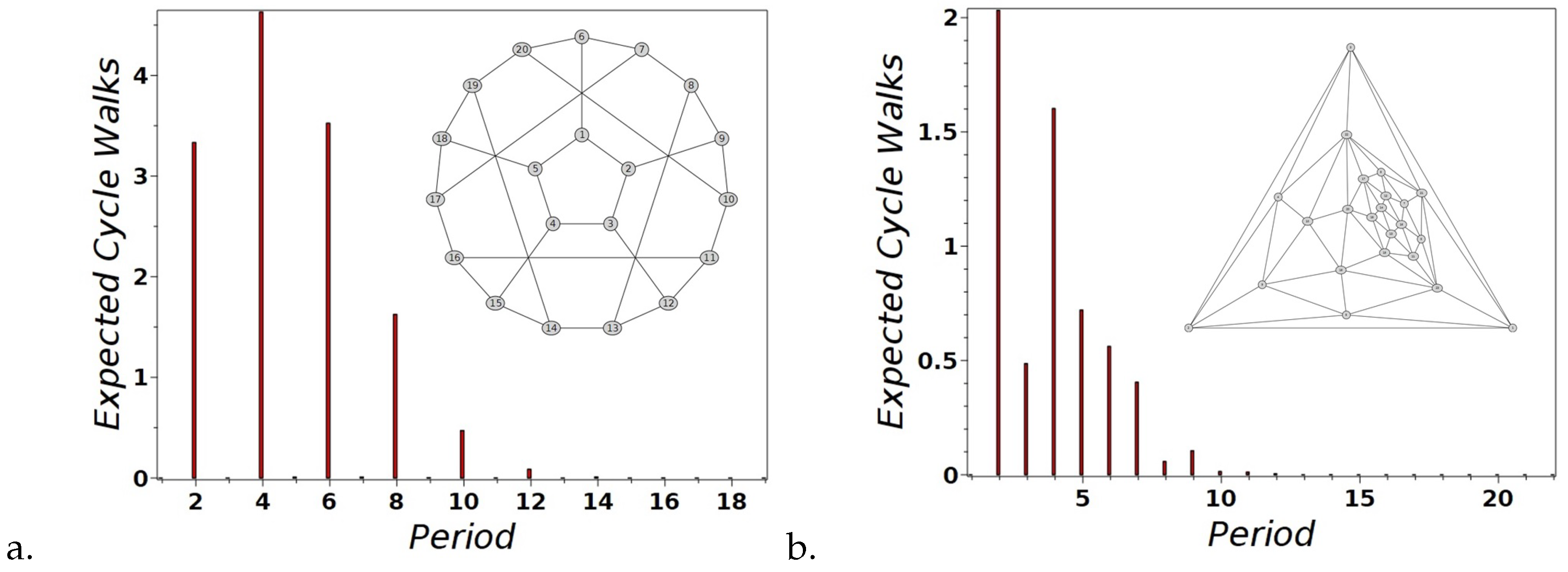
Figure 1. The expected numbers of cycle walks a walker performs in (a) Flower snark graph and (b) Kittell graph per N steps (the graph size).
Dynamics 02 00013 g001
Figure 2. A triangle graph.
Dynamics 02 00013 g002
Figure 3. (a) The stationary densities over the pairs of indices possible on a triangle structure. The pairs of indices are highlighted by color and width in accordance with the corresponding stationary probabilities in (21)–(26). (b) The matrixplot of entropy values for the six diagrams shown in the left panel of the figure. The vertical bars are colored in relation to to the pairs of indices (irrelevant to the probability values in the left panel).
Dynamics 02 00013 g003
Figure 4. The radar graphs representing information decomposition for two canonical ensembles of walks defined by W ( 1 ) and W ( ) , respectively, in (a) the Banana tree graph and in (b) the Flower snark graph.
Dynamics 02 00013 g004
Figure 5. The radar graphs representing information decomposition for two canonical ensembles of walks in the Markov models of the following musical pieces: (a) W.A. Mozart, “Eine Kleine Nachtmusik” (K.525) and (b) R. Wagner, “Das Rheingold” (WWV 86A), the Prelude and Entrance of Gods into Valhalla.
Dynamics 02 00013 g005
Figure 6. The vertices of a membrane graph are highlighted accordingly their (a) Eigenvector centrality, (b) Fugacity.
Dynamics 02 00013 g006
Figure 7. The vertices of Minnesota Road Network are highlighted accordingly their (a) Eigenvector centrality, (b) Fugacity.
Dynamics 02 00013 g007
Table 1. The major differences between CNT and DCN.
CNTDCN
Thermodynamic limitInfinite graphs, N Infinite walks, n
DynamicsEternal growthRandom structural modifications
StatisticsBose-EinsteinFermi–Dirac
Important nodesHigh centrality/ fitnessHigh fugacity
Graph evolution by natural selectionStabilizing selectionDiversifying selection
Table 2. The orthonormal eigenvectors of transition matrix.
Vertex 1Vertex 2Vertex 3
λ = 1 0.57735 0.57735 0.57735
λ = 1 / 2 0.44988 0.81503 0.36515
λ = 1 / 2 0.68138 0.04892 0.73030
Publisher’s Note: MDPI stays neutral with regard to jurisdictional claims in published maps and institutional affiliations.