Communication

On the Zero-Neutron Density in Stochastic Nuclear Dynamics

Department of Mathematics, University of the Basque Country (UPV/EHU), Apto 644, 48080 Bilbao, Spain
Dynamics 2021, 1(2), 198-203; https://doi.org/10.3390/dynamics1020012
Submission received: 28 July 2021 / Revised: 29 September 2021 / Accepted: 22 October 2021 / Published: 4 November 2021

Abstract

:
In this short paper, we compare the deterministic model for the nuclear reactor dynamic (Hetrick, 1993) with the stochastic model (Kinard and Allen, 2004). Our numerical results show coincidences between the deterministic model and the mean of the stochastic paths, although, as already observed by other authors, there is alarge amount of dispersion between the individual paths. Notably, we always observe that the neutron density approaches zero within a short time. In this paper, we investigate this question; more concretely, we study the mean-extinction of the neutron density. The technique used here first builds the backward Kolmogorov differential equation and then solves it numerically using the finite-element method with FreeFem++. Our results confirm that in a very short time the neutrons disappear although later they recover probably due to the external source.

In this paper, we research the time-dependency of a nuclear reactor. Previous models in nuclear reactor dynamics are investigated in [1,2]. We aim to determinate the time behavior of the power level of a nuclear reactor to obtain better control over it, for example, by using the control rod position. The deterministic models explained in [3] or [4] build one-group, time-dependent diffusion equations. The literature that has studied their solutions and their numerical simulation is very extensive, as can be seen in the references of [4]. A few years later, J.G Hayes and E.J. Allen in [5] built a stochastic model, which is explained below. J.G Hayes and E.J. Allen consider the simplest case of a single precursor, while the determinist models assume m type of precursors; moreover, they assume that the nuclear reactor is large and homogeneous, so that spatial effects can be ignored. Then, they have two variables, n ( t ) and c ( t ) , representing neutron and precursor densities, respectively.
In this way, considering a very small time-interval t , such that the probability of more than one event occurring during t is very small, they assume that the changes and their probabilities regarding the first order are given in Table 1 with x = ( n , c ) T .
The physical parameters are as follows:
  • b the neutron birth rate due to fission;
  • d the neutron death rate due to fission;
  • ν the total number of neutrons per fission: ( 1 β ) ν prompt and β ν delayed;
  • λ the constant of fission product c ( t ) ;
  • β ν the number of atoms of fission product c ( t ) produced per fission;
  • q is the extraneous neutron sources.
Fixing x ( t ) at time t, we calculate the expected change for the change x = ( n , c ) T
E ( X ) = j = 1 5 p j X ( j ) = A n ( t ) c ( t ) + q 0 t ,
where
A = ( ( 1 β ) ν 1 ) b d λ β ν b λ ,
and the covariance matrix
E ( x ( x ) T ) = j = 1 5 p j ( x ( j ) ) ( x ( j ) ) T = D ( n , c ) t ,
such that
D ( n , c ) = ( ( 1 β ) ν 1 ) 2 b + d n + λ c + q β ν ( ( 1 β ) ν 1 ) b n λ c β ν ( ( 1 β ) ν 1 ) b n λ c β 2 ν 2 b n + λ c .
Finally we obtain the following Stochastic Differential System (SDE)
d n ( t ) c ( t ) = A n ( t ) c ( t ) + q 0 d t + D 1 / 2 d W 1 ( t ) W 2 ( t ) .
The deterministic nuclear model for two variables n ( t ) and c ( t ) is the linear Ordinary Differential Equations (EDOs)
d n ( t ) d t = ( ( 1 β ) ν 1 ) b d n ( t ) + λ c ( t ) + q , d c ( t ) d t = β ν b n ( t ) λ c ( t ) ,
with a fix-point in
q d + ( 1 ν ) b , β ν q b λ d + ( 1 ν ) b ,
whose stability depends on its Jacobin’s eigenvalues. We can find these using the symbolic manipulator of MATLAB, although it has a complicated expression.
Let us consider the two following examples.
Case 1:
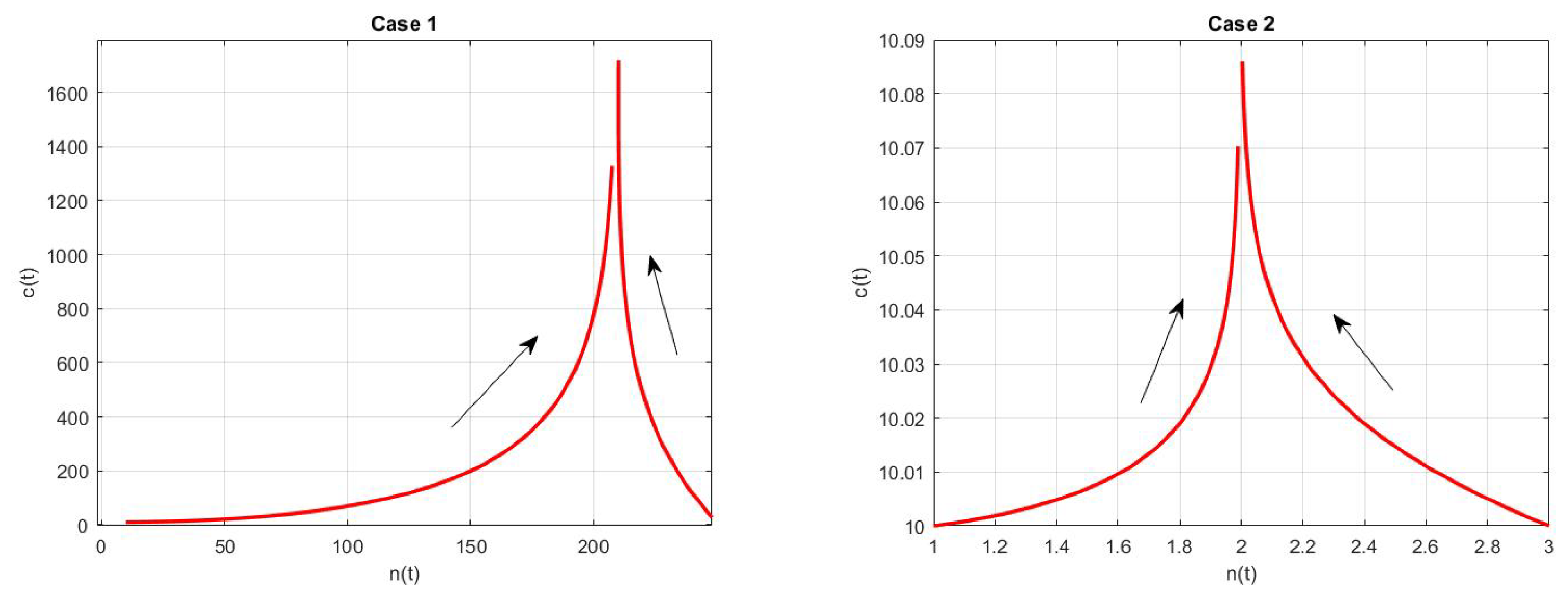
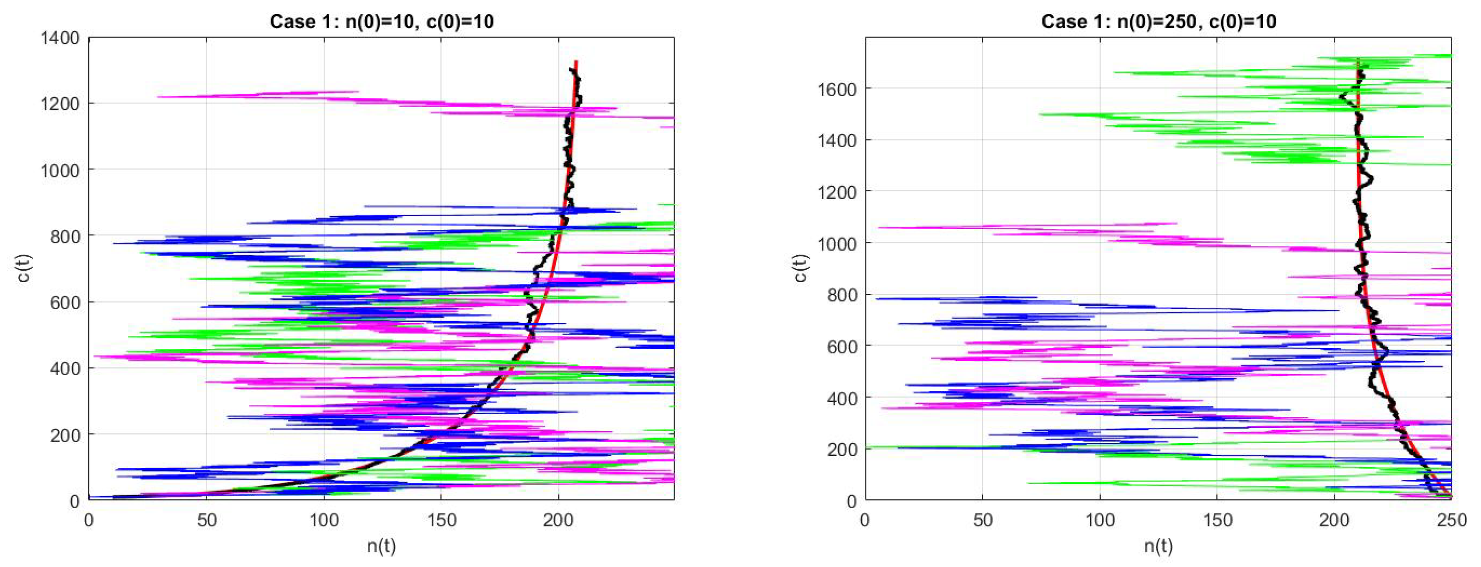
As in the first numerical case, we consider the example in [6], p. 163, with
λ = 0.077 / s e c , β = 0.0079 , ν = 2.432 , b = 4111.84 / s , d = 5858.16 / s , q = 10 , 000 / s ,
which are values for a nuclear reactor involving the thermal fission of uranium-235 in [3]. For these values, the deterministic model (6) has a fixed point at 10 5 × ( 0.0033 , 3.3772 ) and its Jacobian has eigenvalues of 0.0480 and 48.1301 , so the fixed point is unstable. In Figure 1, we plot the numerical solution with Matlab for n ( 0 ) = c ( 0 ) = 10 and n ( 0 ) = 250 , c ( 0 ) = 10 , 0 t 0.1 . (We refer to [7,8,9,10] for a review of the numerical solutions of ODEs).
Case 2:
In the second example, we change the parameter ν = 2.432 / 2 to modify the asymptotic behavior of (6). When the fixed point is 10 3 × ( 0.0020 , 1.0191 ) and the spectrum of the Jacobian is 5009.0 and 1.01 , then the fixed point is an attractor of the linear system. In Figure 1, we plot the numerical solution for n ( 0 ) = 1 , c ( 0 ) = 10 and n ( 0 ) = 3 , c ( 0 ) = 10 , 0 t 0.001 .
Our numerical simulations for stochastic model (5) were performed using the classic Euler–Maruyama numerical method, although it has a strong order 1/2 and weak order 1 (we refer to [11,12,13,14] and, more recently, Ref. [15] for a review on the numerical solutions of SDEs). Thus, we have
n ( t + t ) c ( t + t ) = n ( t ) c ( t ) + A n ( t ) c ( t ) t + q 0 t + D 1 / 2 t η 1 η 2 ,
where η 1 , η 2 N ( 0 , 1 ) . For each step, we have to compute the matrix D 1 / 2 . At this point, we have two options: it is well-known that a positive definite matrix has a unique positive definite matrix square root, and can be caluclated for a 2 × 2 matrix ([6], Remark 5.3). The other option uses the command sqrtm of Matlab. The results are the same, although the second can be applied to any dimension.
In Figure 2 we plot case 1. The deterministic solution is shown in red, the mean of 1000 trials is given in black, and tree sample paths are shown in green, blue and magenta. The step size is t = 10 4 for n ( 0 ) = 10 , c ( 0 ) = 10 on the left and n ( 0 ) = 250 , c ( 0 ) = 10 on the right. These numerical results confirm the observations in Figure 5.7 in ([6], p. 164), Figure 1 in [5] and Figure 1 in [13]: the means are close to the deterministic model, but with very important deviations; in other words, a sample path can be very far from that mean. One of the two variables could even reach very small values, close to zero. This same situation is observed in case 2, on which we do not believe it is necessary to comment.
In the previous figures, we were surprised to see that the paths became very close to zero in a very short time. To understand this behavior, we researched a new random variable T defining the persistence time, i.e., the time it takes for the size of either variables to reach zero.
T inf { t 0 : n ( t ) = 0 or c ( t ) = 0 } ,
obviously, T depends on the initial values n ( 0 ) ) and c ( 0 ) , although this is not explicitly indicated. As the mean persistence-time τ E ( T ) for (5) satisfies the stationary backward Kolmogorov equation (see, for example, ([6], p. 150), [16,17,18]), then, if we name n ( 0 ) = x and c ( 0 ) = y , this partial differential equation is
μ 1 ( x , y ) τ x + μ 2 ( x , y ) τ y + 1 2 d 11 ( x , y ) 2 τ x 2 2 d 12 ( x , y ) 2 τ x y + d 22 ( x , y ) 2 τ y 2 = 1 ,
where
μ 1 ( x , y ) = ( ( 1 β ) ν 1 ) b d x + λ y + q , , μ 2 ( x , y ) = β ν b x λ y ,
and the boundary conditions are
τ ( 0 , x ) = τ ( y , 0 ) = 0 , τ x ( M x , y ) = 0 , τ y ( x , M y ) = 0 ,
provided that the number of x and y cannot exceed some values, such as M x and M y , respectively.
The Finite-Element Method (FEM) is a classic method for the numerical solution of partial derivative equations (PDE). These techniques are explained in any introductory course in the numerical solution of PDE. There is an ample bibliography about FEMs and their implementation (see, for instance, [19] for a very clear introduction).
To resolve the boundary problems (9) and (10) using the FEM, let us multiply (9) by a regular function ϕ ( x , y ) , satisfying the homogeneous Dirichlet boundary conditions. After integrating these over the domain Ω = [ 0 , M x ] × [ 0 , M y ] , the following terms will appear:
Ω d 11 2 τ x 2 ϕ = Ω d 11 τ x ϕ x Ω d 11 x τ x ϕ + 0 M y τ x · d 11 · ϕ ( M x , y ) d y , Ω d 22 2 τ y 2 ϕ = Ω d 22 τ y ϕ y Ω d 22 y τ y ϕ + 0 M x τ y · d 22 · ϕ ( x , M y ) d x , Ω d 12 2 τ x y ϕ = Ω d 12 τ y ϕ x + Ω d 12 x τ y ϕ 0 M y τ y · d 12 · ϕ ( M x , y ) d y .
such that from (10)
0 M y τ x · d 11 · ϕ ( M x , y ) d y = 0 M x τ y · d 22 · ϕ ( x , M y ) d x = 0 .
We computed the FEM solution of (9) and (10) with M x = 300 , M y = 100 using FreeFem++, with the result shown in Figure 3. From these results, we highlight the following: For this set of initial values: 0 < n ( 0 ) < 300 , 0 < c ( 0 ) < 100 , the mean time for the number of neutrons to reach zero is less than a tenth; more specifically, as we can see from Figure, τ ( 10 , 10 ) 0.0703856 and τ ( 250 , 10 ) 0.0853348 . These results explain our previous observations.

Conclusions

Our main conclusion is that the deterministic solutions and mean of stochastic solution averages are very close, but, in a very short time, the neutrons disappear. However, they recover quickly, probably due to the external source. To test this assumption, we consider q = 100 . In Figure 4, on the left, we plot n ( 0 ) = 10 ; c ( 0 ) = 10 : the deterministic solution is given in red, the mean of 1000 trials in black, and tree sample paths in green, blue and magenta in 0 t 0.1 . On the right, the numerical solution of (9) and (10) with M x = 100 , M y = 100 is shown. These results suggest that when the source is reduced, the stochastic model moves away from the deterministic one and, above all, the neutrons disappear much earlier.
However, in [20,21] an alternative stochastic formulation was proposed based on the classical Chemical Calgevin Method (e.g., [22,23,24,25]). However, in my opinion this statement is not correct. In remark 5.4 from ([6], p. 143) or [26], it is shown that the both models are the same.

Funding

This work was supported by Spanish Ministry of Sciences Innovation and Universities with the project PGC2018-094522-B-100 and by the Basque Government with the project IT1247-19.

Institutional Review Board Statement

Not applicable.

Informed Consent Statement

Not applicable.

Data Availability Statement

The numerical methods were implemented in Matlab© and FreeFem++ which is freely available [27]. The experiments were carried out in an Intel(R) Core(TM)i7-8665U CPU @ 1.90 GHz, 16.0 GB of RAM. The codes for the numerical tests are available on request.

Acknowledgments

The author would like to thank the referees for the constructive and helpful comments and suggestions on the manuscript.

Conflicts of Interest

The author declares no conflict of interest.

References

  1. Hetrick, D. Dynamics of Nuclear Reactors; American Nuclear Sociaty: La Grange Park, IL, USA, 1993. [Google Scholar]
  2. Kinard, M.; Allen, E. Efficient numerical solution of the point kinetics equations in nuclear reactor dynamics. Ann. Nucl. Energy 2004, 31, 1039–1051. [Google Scholar] [CrossRef]
  3. Hetrick, D. Dynamics of Nuclear Reactors; University of Chicago: Chicago, IL, USA, 1971. [Google Scholar]
  4. Stacey, W. Nuclear reactor Physics, 2nd ed.; Completety Revised and Enlarged; WILEY-VCG Verlag GmbH & Co. KGaA: Weinheim, Germany, 2007. [Google Scholar]
  5. Hayes, J.; Allen, E. Stochastic point-kinetics equations in nuclear reactor dynamics. Ann. Nucl. Energy 2005, 32, 572–587. [Google Scholar] [CrossRef] [Green Version]
  6. Allen, E. Modeling with Itô Stochastic Differential Equations; Springer: Berlin/Heidelberg, Germany, 2007. [Google Scholar]
  7. Higham, D.; Higham, N. MATLAB Guide; SIAM: Philadelphia, PA, USA, 2000. [Google Scholar]
  8. Shampine, L.; Gladwell, I.; Thompson, S. Solving ODEs with MATLAB; Cambridge University Press: Cambridge, UK, 2003. [Google Scholar]
  9. Moler, C. Numerical Computing with MATLAB; SIAM: Philadelphia, PA, USA, 2004. [Google Scholar]
  10. Sharin, M. Exploration of Mathematical Models in Biology with MATLAB; Wiley: Hoboken, NJ, USA, 2014. [Google Scholar]
  11. Kloeden, P.; Platen, E. Numerical Solution of Stochastic Differential Equations; Cambridge University Press: Cambridge, UK, 1998. [Google Scholar]
  12. Higham, D. An Algorithmic Introduction to Numerical Simulation of Stochastic Differential Equations. SIAM Rev. 2001, 43, 525–546. [Google Scholar] [CrossRef]
  13. Ray, S. Numerical simulation of stochastic point kinetic equation in the dynamical system of nuclear reactor. Ann. Nucl. Energy 2012, 49, 154–159. [Google Scholar]
  14. Suescún-Díaz, D.; Oviedo-Torres, Y.; Girón-Cruz, L. Solution of the stochastic point kinetics equations using the implicit Euler-Maruyama method. Ann. Nucl. Energy 2018, 117, 45–52. [Google Scholar] [CrossRef]
  15. Higham, D.; Kloeden, E. An Introduction to the Numerical Simulation of Stochastic Differential Equations; SIAM: Philadelphia, PA, USA, 2021. [Google Scholar]
  16. de la Hoz, F.; Vadillo, F. A mean extinction-time estimate for a stochastic Lotka-Volterra predator-prey model. Appl. Math. Comput. 2012, 219, 170–179. [Google Scholar] [CrossRef]
  17. Doubova, A.; Vadillo, F. Extinction-time for stochastic population models. J. Comput. Appl. Mathemtics 2016, 295, 159–169. [Google Scholar] [CrossRef]
  18. Vadillo, F. Comparing stochastic Lotka-Volterra predator-prey models. Appl. Math. Comput. 2019, 360, 181–189. [Google Scholar] [CrossRef]
  19. Gockenbach, M. Understanding and Implementing the Finite Element Method; SIAM: Philadelphia, PA, USA, 2006. [Google Scholar]
  20. Ayyoubzadeh, S.M.; Vosoughi, N. An alternative stochastic formulation for the point reactor. Ann. Nucl. Energy 2014, 63, 691–695. [Google Scholar] [CrossRef]
  21. Elsayed, A.; El-Beltagy, M.; Al-Juhani, A.; Al-Qahtani, S. A New Model for the Stochastic Point Reactor: Development and Comparison with Available Models. Energies 2021, 14, 955. [Google Scholar] [CrossRef]
  22. Gillespie, D. Approximate accelerated stochastic simulation of chemically. J. Chem. Phys. 2001, 115, 1716–1733. [Google Scholar] [CrossRef]
  23. Gillespie, D. The Chemical Langevin and Fokker-Planck Equations for the Reversible Isomerization Reaction. J. Phys. Chem. 2002, 106, 5063–5071. [Google Scholar] [CrossRef]
  24. Gillespie, D.; Petzold, L. Numerical simulation for biochemical kinetics. In System Modeling in Cellular Biology From Concepts to Nuts and Bolts; Szallasi, Z., Stelling, J., Periwal, V., Eds.; MIT Press: Cambridge, MA, USA, 2006; pp. 331–353. [Google Scholar]
  25. Schilick, T. Molecular Modeling and Simulation. An Interdisciplinary Guide, 2nd ed.; Springer: Berlin/Heidelberg, Germany, 2010. [Google Scholar]
  26. Vadillo, F. On Stochastic Models of Chemical Reactions. Chem. Phys. 2021, 549, 111259. [Google Scholar] [CrossRef]
  27. Hecht, F. New development in freefem++. J. Numer. Math. 2012, 20, 251–265. [Google Scholar] [CrossRef]
Figure 1. The numerical solution of deterministic mode case 1 is shown on the left, with n ( 0 ) = c ( 0 ) = 10 and n ( 0 ) = 250 , c ( 0 ) = 10 , for 0 t 0.1 . On the right, case 2 is shown, with n ( 0 ) = 1 , c ( 0 ) = 10 and n ( 0 ) = 3 , c ( 0 ) = 10 , for 0 t 0.001 .
Dynamics 01 00012 g001
Figure 2. The numerical solution of stochastic mode case 1. The deterministic solution, is shown in red, the mean of 1000 trials in black, and tree sample paths in green, blue and magenta.
Dynamics 01 00012 g002
Figure 3. Numerical solution of (9)–(10) with M x = 300 , M y = 100 .
Dynamics 01 00012 g003
Figure 4. On the left, for n ( 0 ) = 10 ; c ( 0 ) = 10 : the deterministic solution is shown in red, the mean of 1000 trials in black, and tree sample paths in green, blue and magenta in 0 t 0.1 . On right the numerical solution of (9) and (10) with M x = 100 , M y = 100 .
Dynamics 01 00012 g004
Table 1. Possible change in x = ( n , c ) T .
ChangeProbability
x ( 1 ) = [ 1 , 0 ] T p 1 = q t
x ( 2 ) = [ 1 , 0 ] T p 2 = d n ( t ) t
x ( 3 ) = [ 1 , 1 ] T p 3 = λ c ( t ) t
x ( 4 ) = [ ( 1 β ) ν 1 , β ν ] T p 4 = b n ( t ) t
x ( 5 ) = [ 0 , 0 ] T p 5 = 1 i = 1 4 p i
Publisher’s Note: MDPI stays neutral with regard to jurisdictional claims in published maps and institutional affiliations.

