Entropy

Definition

The concept of entropy constitutes, together with energy, a cornerstone of contemporary physics and related areas. It was originally introduced by Clausius in 1865 along abstract lines focusing on thermodynamical irreversibility of macroscopic physical processes. In the next decade, Boltzmann made the genius connection—further developed by Gibbs—of the entropy with the microscopic world, which led to the formulation of a new and impressively successful physical theory, thereafter named statistical mechanics. The extension to quantum mechanical systems was formalized by von Neumann in 1927, and the connections with the theory of communications and, more widely, with the theory of information were respectively introduced by Shannon in 1948 and Jaynes in 1957. Since then, over fifty new entropic functionals emerged in the scientific and technological literature. The most popular among them are the additive Renyi one introduced in 1961, and the nonadditive one introduced in 1988 as a basis for the generalization of the Boltzmann–Gibbs and related equilibrium and nonequilibrium theories, focusing on natural, artificial and social complex systems. Along such lines, theoretical, experimental, observational and computational efforts, and their connections to nonlinear dynamical systems and the theory of probabilities, are currently under progress. Illustrative applications, in physics and elsewhere, of these recent developments are briefly described in the present synopsis.

1. Introduction

Thermodynamics is an empirical physical theory which describes relevant aspects of the behavior of macroscopic systems. In some form or another, all large physical systems are shown to satisfy this theory. It is based on two most relevant concepts, namely energy and entropy. The German physicist and mathematician Rudolf Julius Emanuel Clausius (1822–1888) introduced the concept of entropy in 1865 [1,2], along rather abstract lines in fact. He coined the word from the Greek $\tau \rho o\pi \eta$ ($trop\overline{e}$), meaning transformation, turning, change. Clausius seemingly appreciated the phonetic and etymological consonance with the word ’energy’ itself, from the Greek $ϵ\nu ϵ\rho \gamma ϵ\iota \alpha$ ($energeia$), meaning activity, operation, work. It is generally believed that Clausius denoted the entropy with the letter S in honor of the French scientist Sadi Carnot. For a reversible infinitesimal process, the exact differential quantity $dS$ is related to the differential heat transfer $\delta Q_{reversible}$ through $dS=\frac{\delta Q_{reversible}}{T}$, T being the absolute temperature. The quantity $T^{-1}$ plays the role of an integrating factor, which transforms the differential transfer of heat (dependent on the specific path of the physical transformation) into the exact differential quantity of entropy (path-independent). This relation was thereafter generalized by Clausius into its celebrated inequality $dS\ge \delta Q/T$, the equality corresponding to a reversible process. The inequality corresponds to irreversible processes and is directly implied by the so-called Second Principle of Thermodynamics, deeply related to our human perception of the arrow of time.

One decade later, the Austrian physicist and philosopher Ludwig Eduard Boltzmann (1844–1906) made a crucial discovery, namely the connection of the thermodynamic entropy S with the microscopic world [3,4]. The celebrated formula $S=klnW$, W being the total number of equally probable microscopic possibilities compatible with our information about the system, is carved in his tombstone in the Central Cemetery of Vienna. Although undoubtedly Boltzmann knew this relation, it appears that he never wrote it in one of his papers. The American physicist, chemist and mathematician Josiah Willard Gibbs (1839–1903) further discussed and extended the physical meaning of this connection [5,6,7]. Their efforts culminated in the formulation of a powerful theory, currently known as statistical mechanics. This very name was, at the time, a deeply controversial matter. Indeed, it juxtaposes the word mechanics—cornerstone of a fully deterministic understanding of Newtonian mechanics—and the word statistics—cornerstone of a probabilistic description, precisely based on non-deterministic concepts. On top of that, there was the contradiction with the Aristotelian view that fluids, e.g., the air, belong to the mineral kingdom of nature, where there is no place for spontaneous motion. In severe variance, Boltzmann’s interpretation of the very concept of temperature was directly related to spontaneous space-time fluctuations of the molecules (‘atoms’) which constitute the fluid itself.

Many important contributions followed, including those by Max Planck, Paul and Tatyana Ehrenfest, and Albert Einstein himself. Moreover, we mention here an important next step concerning entropy, namely its extension to quantum mechanical systems. It was introduced in 1927 [8] by the Hungarian-American mathematician, physicist and computer scientist János Lajos Neumann (John von Neumann; 1903–1957).

The next nontrivial advance was done in 1948 by the American electrical engineer and mathematician Claude Elwood Shannon (1916–2001), who based on the concept of entropy his “Mathematical Theory of Communication” [9,10,11]. This was the seed of what nowadays is ubiquitously referred to as the information theory, within which the American physicist Edwin Thompson Jaynes (1922–1998) introduced the maximal entropy principle, thus establishing the connection with statistical mechanics [12,13]. Along these lines, several generalizations were introduced, the first of them, hereafter noted $S_q^R$, by the Hungarian mathematician Alfréd Rényi (1921–1970) in 1961 [14,15,16,17]. Various others followed in the next few decades within the realm of information theory, cybernetics and other computer-based frames, such as the functionals by Havrda, Charvat [18], Lindhard, Nielsen [19], Sharma, Taneja, Mittal [20,21,22]. During this long maturation period, many important issues have been punctuated. Let us mention, for instance, Jaynes’ “anthropomorphic” conceptualization of entropy [23] (first pointed by E.P. Wigner), and also Landauer’s “Information is physical” [24]. In all cases, the entropy emerges as a measure (a logarithmic measure for the Boltzmann–Gibbs instance) of the number of states of the system that are accessible, or, equivalently, as a measure of our ignorance or uncertainty about the system.

In 1988, the Greek-Argentine-Brazilian physicist Constantino Tsallis proposed the generalization of statistical mechanics itself on the basis of a nonadditive entropy, noted $S_q$, where the index q is a real number; $S_q$ recovers the Boltzmann–Gibbs (BG) expression for the value $q=1$ [25]. This theory is currently referred to as nonextensive statistical mechanics [26]. There was subsequently an explosion of entropic functionals: there are nowadays over fifty such entropies in the available literature. However, very few among them have found neat applications in physics and elsewhere.

2. Basics

2.1. Definitions and Properties of Entropy

The Boltzmann–Gibbs–von Neumann–Shannon entropic functional (or entropy for simplicity) for discrete variables is defined as follows:

$$S_{BG}\equiv -k\sum _{i=1}^W{p}_{i}ln{p}_i\left(\sum _{i=1}^W{p}_i=1\right),$$

(1)

where k is a conventional positive constant (currently taken to be the Boltzmann constant in physics, and $k=1$ in information theory), and $\left\{p_i\right\}$ are the probabilities corresponding to W possible states.

For classical systems, the discrete index i is replaced by a real continuous variable x, and we have the form that was used by Boltzmann and Gibbs themselves, namely

$$S_{BG}\equiv -k\int dxp\left(x\right)lnp\left(x\right)\left(\int dxp\left(x\right)=1\right).$$

(2)

(Some mathematical care might be necessary in this limiting case; for instance, if the distribution is extremely thin, this classical expression of $S_{BG}$ might lead to unphysical negative values; although not particularly transparent, such difficulties simply disappear if we take into account that the Planck constant is different from zero.)

For quantum systems, we have

$$S_{BG}\equiv -kTr\rho ln\rho \left(Tr\rho =1\right),$$

(3)

where $\rho$ is the density matrix, acting on an appropriate Hilbert space; under this form, $S_{BG}$ is also referred to as von Neumann entropy [8]. Definition (1) can be expressed as a particular instance of (2) through Dirac’s delta distributions (with $p\left(x\right)={\sum }_{i=1}^W\delta (x_i-p_i)$), and also as a particular instance of (3) when $\rho$ is diagonal.

In all cases, we may say that entropy is a logarithmic measure of the lack of information on the system. When we know everything about the state of the system (more precisely, on which one of the possible W states the system is), $S_{BG}$ vanishes. When we know nothing (more precisely, when $p_i=1/W$ for all values of i) $S_{BG}$ attains its maximal value

$$S_{BG}=klnW.$$

(4)

This equality constitutes a crucial connection between the macroscopic world (represented by the thermodynamical entropy $S_{BG}$) and the microscopic world (represented by the total number W of microscopic possibilities).

Let us now address the generalizations of $S_{BG}$ that exist in the literature. Given their enormous amount, we shall restrict ourselves to the two most popular ones after the BG entropy itself, namely the additive Renyi entropy $S_q^R$ [14,15,16,17] and the nonadditive entropy $S_q$ [25]. They are respectively defined as follows, q being a real number:

$$S_q^R\equiv k\frac{ln{\sum }_{i=1}^W{p}_i^q}{1-q}(S_1^R=S_{BG}),$$

(5)

and

$$\begin{array}{ccc}\hfill S_q& \equiv & k\frac{1-{\sum }_{i=1}^W{p}_i^q}{q-1}=k\sum _{i=1}^W{p}_i{ln}_q\frac{1}{p_i}\hfill \\ & =& -k\sum _{i=1}^W{p}_i^q{ln}_q{p}_i=-k\sum _{i=1}^W{p}_i{ln}_{2-q}{p}_i(S_1=S_{BG}),\hfill \end{array}$$

(6)

where the q-logarithmic function is defined through

$${ln}_{q}z\equiv \frac{z^{1-q}-1}{1-q}({ln}_{1}z=lnz).$$

(7)

The quantity $\sigma \left(p\right)\equiv ln(1/p)$ is referred to as surprise [27] or unexpectedness [28]. It vanishes when the probability p equals unity, and diverges when the probability $p\to 0$. We can consistently define q-surprise or q-unexpectedness as ${\sigma }_q\left(p\right)\equiv {ln}_q(1/p)$, hence ${\sigma }_q\left(1\right)=0$ and ${\sigma }_q\left(0\right)$ diverges. With this definition, $S_q$ can be rewritten in the following way:

$$S_q=k\sum _{i=1}^W{p}_i{ln}_q(1/p_i)\equiv ⟨{ln}_q(1/p_i)⟩=⟨{\sigma }_q⟩,$$

(8)

where $⟨\cdots ⟩$ denotes the mean value.

It can be verified that

$$S_q^R/k=\frac{ln[1+(1-q)S_q/k]}{1-q},$$

(9)

which implies that $S_q^R$ monotonically increases with $S_q$ (like, say, ${\left(S_{BG}\right)}^3$ monotonically increases with $S_{BG}$). Moreover, it can be shown that $S_q\left(\left\{p_i\right\}\right)$ is concave for $q>0$, and convex for $q<0$, whereas $S_q^R$ is concave for $0<q\le 1$, convex for $q<0$, and neither concave nor convex for $q>1$. They both attain, for equal probabilities, their extremal value (maximal for $q>0$, and minimal for $q<0$), namely

$$S_q^R=klnW,$$

(10)

and

$$S_q=k{ln}_{q}W.$$

(11)

2.2. Additivity versus Extensivity

We address now two important notions, namely entropic additivity and extensivity. Following O. Penrose [29], an entropic functional $S\left(\left\{p_i\right\}\right)$ is said additive if, for two probabilistically independent systems A and B (i.e., $p_{ij}^{A+B}=p_i^A{p}_j^B)$, we verify $S(A+B)=S\left(A\right)+S\left(B\right)$, in other words, if we verify that

$$S\left(\left\{p_{i,j}^{A+B}\right\}\right)=S\left(\left\{p_i^A\right\}\right)+S\left(\left\{p_j^B\right\}\right).$$

(12)

Otherwise, $S\left(\left\{p_i\right\}\right)$ is said nonadditive. It immediately follows that $S_{BG}$ and $S_q^R$ (for all values of q) are additive. In contrast, $S_q$ satisfies

$$\frac{S_q(A+B)}{k}=\frac{S_q\left(A\right)}{k}+\frac{S_q\left(B\right)}{k}+(1-q)\frac{S_q\left(A\right)}{k}\frac{S_q\left(B\right)}{k},$$

(13)

hence

$$S_q(A+B)=S_q\left(A\right)+S_q\left(B\right)+\frac{1-q}{k}{S}_q\left(A\right)S_q\left(B\right).$$

(14)

Therefore, unless $(1-q)/k\to 0$, $S_q$ is nonadditive.

Let us briefly mention at this point a simple generalization of $S_q$ which appears to be convenient for some specific purposes, such as black holes, cosmology, and possibly other physical systems. We define [30]

$$S_{q,\delta }\equiv k\sum _{i=1}^W{p}_i{\left[{ln}_q\frac{1}{p_i}\right]}^{\delta }.$$

(15)

We can verify that $S_{1,1}=S_{BG}$, $S_{q,1}=S_q$, and $S_{1,\delta }=S_{\delta }$ where [26,31]

$$S_{\delta }\equiv k\sum _{i=1}{p}_i{\left[ln\frac{1}{p_i}\right]}^{\delta }.$$

(16)

Various properties of the nonadditive entropy $S_{q,\delta }$ are discussed in [32].

Let us now address the other important entropic concept, namely extensivity. An entropy $S\left(N\right)$ is said extensive if a specific entropic functional is applied to a many-body system with $N=L^d$ particles, where L is its dimensionless linear size and d its spatial dimension, and satisfies the thermodynamical expectation

$$0<\underset{N\to \infty }{lim}\frac{S\left(N\right)}{N}<\infty ,$$

(17)

hence $S\left(N\right)\propto N$ for $N\gg 1$. Therefore, entropic additivity only depends on the entropic functional, whereas entropic extensivity depends on both the chosen entropic functional and the system itself (its constituents and the correlations among them).

Let us illustrate this distinction through four, among infinitely many, equal-probability typical examples of $W\left(N\right)(N\to \infty )$, where W is the total number of possibilities whose probability does not vanish.

• Exponential class $W\left(N\right)\sim A{\mu }^N(A>0;\mu >1)$:
  This is the typical case within the BG theory. We have $S_{BG}\left(N\right)=klnW\left(N\right)\sim Nln\mu +lnA\propto N$, therefore $S_{BG}$ is extensive, as thermodynamically required.
• Power-law class $W\left(N\right)\sim B{N}^{\rho }(B>0;\rho >0)$:
  We should not use $S_{BG}$ since it implies $S_{BG}\left(N\right)=klnW\left(N\right)\sim \rho lnN+lnB\propto lnN$, thus violating thermodynamics. We verify instead that $S_{q=1-1/\rho }\left(N\right)=k{ln}_{q=1-1/\rho }W\left(N\right)\propto N$, as thermodynamically required.
• Stretched exponential class $W\left(N\right)\sim C{\nu }^{N^{\gamma }}(C>0;\nu >1;0<\gamma <1)$:
  In this instance, no value of q exists which would imply an extensive entropy $S_q$. We can instead used $S_{\delta }$ with $\delta =1/\gamma$. Indeed, $S_{\delta =1/\gamma }\left(N\right)=k{[lnW\left(N\right)]}^{\delta }\propto N$, as thermodynamically required.
• Logarithmic class $W\left(N\right)\sim DlnN(D>0)$:
  In this case, no values of $(q,\delta )$ exist which imply an extensive entropy $S_{q,\delta }$. Instead, we can use the Curado entropy [33] $S_{\lambda }^C\left(N\right)=k\left[e^{\lambda W\left(N\right)}-e^{\lambda }\right]$ with $\lambda =1/D$. Indeed, we can verify that $S_{\lambda =1/D}^C\left(N\right)\propto N$, as thermodynamically required.

These four paradigmatic cases are indicated in Figure 1.

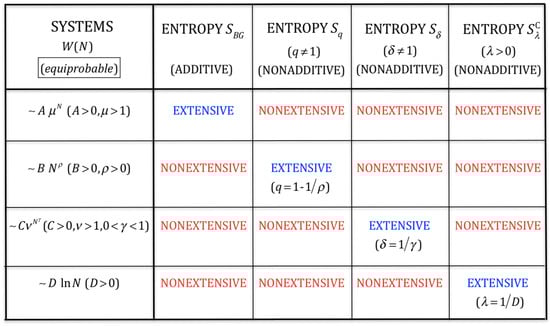
Figure 1. Typical behaviors of $W\left(N\right)$ (number of nonzero-probability states of a system with N random variables) in the $N\to \infty$ limit and entropic functionals which, under the assumption of equal probabilities for all states with nonzero probability, yield extensive entropies for specific values of the corresponding (nonadditive) entropic indices. In what concerns the exponential class $W\left(N\right)\sim A{\mu }^N$, $S_{BG}$ is not the unique entropy that yields entropic extensivity; the (additive) Renyi entropic functional $S_q^R$ also is extensive for all values of q. Analogously, in what concerns the stretched-exponential class $W\left(N\right)\sim C{\nu }^{N^{\gamma }}$, the (nonadditive) entropic functional $S_{\delta }$ is not unique. All the entropic families illustrated in this table contain $S_{BG}$ as a particular case, except $S_{\lambda }^C$, which is appropriate for the logarithmic class $W\left(N\right)\sim DlnN$. In the limit $N\to \infty$, the inequalities ${\mu }^N\gg {\nu }^{N^{\gamma }}\gg N^{\rho }\gg lnN\gg 1$ are satisfied, hence ${lim}_{N\to \infty }{\nu }^{N^{\gamma }}/{\mu }^N={lim}_{N\to \infty }{N}^{\rho }/{\mu }^N={lim}_{N\to \infty }lnN/{\mu }^N=0$. This exhibits that, in all these nonadditive cases, the occupancy of the full phase space corresponds essentially to zero Lebesgue measure, similarly to a whole class of (multi) fractals. If the equal probabilities hypothesis is not satisfied, specific analysis becomes necessary and the results might be different.

It is pertinent to remind, at this point, Einstein’s 1949 words [34]: “A theory is the more impressive the greater the simplicity of its premises is, the more different kinds of things it relates, and the more extended is its area of applicability. Therefore the deep impression that classical thermodynamics made upon me. It is the only physical theory of universal content concerning which I am convinced that, within the framework of applicability of its basic concepts, it will never be overthrown”.

To better understand the strength of these words, a metaphor can be used. Within Newtonian mechanics, we have the well-known Galilean composition of velocities $v_{13}=v_{12}+v_{23}$. In special relativity, this law was generalized into $v_{13}=[v_{12}+v_{23}]/[1+v_{12}{v}_{23}/c^2]$. Why did Einstein abandon the simple linear composition of Galileo? Because he had a higher goal, namely to unify mechanics and Maxwell electromagnetism, and, for this, he had to impose the invariance with regard to the Lorentz transformation. We may thus see the violation of the linear Galilean composition as a small price to pay for a major endeavor. Analogously, what is expressed in Figure 1, is that generalizing the linear composition law of $S_{BG}$ with regard to independent systems into the nonlinear composition (13) may be seen as a small price to pay for a major endeavor, namely to always satisfy the Legendre structure of thermodynamics. However, it is mandatory to register here that such a viewpoint is nevertheless not free from controversy, in spite of its simplicity. For example, the well-known expression of Bekenstein and Hawking for the entropy for a black hole is proportional to its surface instead of to its volume, therefore violating the above requirement.

2.3. Range of Interactions

Let us consider a d-dimensional classical many-body system with say attractive two-body isotropic interactions decaying with a dimensionless distance $r\ge 1$ as $-A/r^{\alpha }$ ($A>0$, $\alpha \ge 0$), and with a infinitely repulsive potential for $0\le r\le 1$. At zero temperature T, the total kinetic energy vanishes, and the potential energy per particle is proportional to ${\int }_1^{\infty }dr{r}^d{r}^{-\alpha }$. This quantity converges if $\alpha /d>1$ and diverges otherwise. These two regimes are from now on respectively referred to as short-range and long-range interactions: see Figure 2.

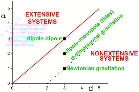
Figure 2. The classical systems for which $\alpha /d>1$ correspond to an extensive total energy and typically involve absolutely convergent series, whereas the so-called nonextensive systems ($0\le \alpha /d<1$ for the classical ones) correspond to a superextensive total energy and typically involve divergent series. The marginal systems ($\alpha /d=1$ here) typically involve conditionally convergent series, which therefore depend on the boundary conditions, i.e., typically on the external shape of the system. Capacitors constitute a notorious example of the $\alpha /d=1$ case. The model usually referred to in the literature as the Hamiltonian-Mean-Field (HMF) one [35] lies on the $\alpha =0$ axis (for all values of $d>0$). The models usually referred to as the d-dimensional $\alpha$-XY [36], $\alpha$-Heisenberg [37,38,39] and $\alpha$-Fermi–Pasta–Ulam (or $\alpha$-Fermi–Pasta–Ulam–Tsingou problem [40,41]) [42,43,44] models lie parallel to the vertical axis at abscissa d (for all values of $\alpha \ge 0$). The standard Lennard–Jones gas is located at $(d,\alpha )=(3,6)$. From [33].

In addition, they can be shown to respectively correspond, within the BG theory, to finite and divergent partition functions. This is precisely the point that was addressed by Gibbs himself [5,6,7]: “In treating of the canonical distribution, we shall always suppose the multiple integral in Equation (92) [the partition function, as we call it nowadays] to have a finite value, as otherwise the coefficient of probability vanishes, and the law of distribution becomes illusory. This will exclude certain cases, but not such apparently, as will affect the value of our results with respect to their bearing on thermodynamics. It will exclude, for instance, cases in which the system or parts of it can be distributed in unlimited space [...]. It also excludes many cases in which the energy can decrease without limit, as when the system contains material points which attract one another inversely as the squares of their distances [...]. For the purposes of a general discussion, it is sufficient to call attention to the assumption implicitly involved in the formula (92)”.

The standard BG recipe demands integration up to infinity in ${\int }_1^{\infty }dr{r}^d{r}^{-\alpha }$. In slight variance, let us assume that the N-particle system is roughly homogeneously distributed within a limited sphere. Then, the potential energy per particle scales as follows:

$$\frac{U_{pot}\left(N\right)}{N}\propto -A{\int }_1^{N^{1/d}}dr{r}^{d-1}{r}^{-\alpha }=-\frac{A}{d}{N}^{*},$$

(18)

with

$$N^{☆}\equiv \frac{N^{1-\alpha /d}-1}{1-\alpha /d}={ln}_{\alpha /d}N\sim \left\{\begin{array}{ccc}{\displaystyle \frac{1}{\alpha /d-1}}\hfill & \hfill & \mathrm{if}\alpha /d>1;\hfill \\ \\ lnN\hfill & \hfill & \mathrm{if}\alpha /d=1;\hfill \\ \\ {\displaystyle \frac{N^{1-\alpha /d}}{1-\alpha /d}}\hfill & \hfill & \mathrm{if}0<\alpha /d<1.\hfill \end{array}\right.$$

(19)

Therefore, in the $N\to \infty$ limit, $\frac{U_{pot}\left(N\right)}{N}$ approaches a constant ($\propto -A/(\alpha -d)$) if $\alpha /d>1$, and diverges like $N^{1-\alpha /d}/(1-\alpha /d)$ if $0\le \alpha /d<1$ (it diverges logarithmically if $\alpha /d=1$). In other words, the total potential energy is extensive for short-range interactions ($\alpha /d>1$), and nonextensive for long-range interactions ($0\le \alpha /d\le 1$). Equation (19) recovers the characterization with ${\int }_1^{\infty }dr{r}^d{r}^{-\alpha }$ in the limit $N\to \infty$. They have, however, the great advantage of providing a finite value for finite N. This fact will be now shown to enable a proper scaling for the macroscopic quantities in the thermodynamic limit ($N\to \infty$) for all values of$\alpha /d\ge 0$, and not only for $\alpha /d>1$.

2.4. Thermodynamics and Legendre Transformations

The mathematical structure of classical thermodynamics is based on the Legendre transforms. It is not sufficiently realized that thermodynamics does not depend from microscopic details only for short-range interactions. As we illustrate here below, it does depend on quantities such as $(\alpha ,d)$ for long-range interactions. In Landsberg’s words [45,46]: “The presence of long-range forces causes important amendments to thermodynamics, some of which are not fully investigated as yet”.

Let us consider now an illustrative d-dimensional homogeneous and isotropic classical fluid containing magnetic particles in thermodynamical equilibrium. Its Gibbs free energy is then given by

$$\begin{array}{ccc}\hfill G(N,T,p,\mu ,H)& =& U(N,T,p,\mu ,H)-TS(N,T,p,\mu ,H)\hfill \\ & +& pV(N,T,p,\mu ,H)-\mu N-HM(N,T,p,\mu ,H),\hfill \end{array}$$

(20)

where $(T,p,\mu ,H)$ correspond respectively to the temperature, pressure, chemical potential and external magnetic field, U is the internal energy, S is the entropy, V is the volume, N is the number of particles and M the magnetization.

If the interactions are short-ranged, i.e., if $\alpha /d>1$, we can divide this equation by N and then take the $N\to \infty$ limit. We obtain

$$g(T,p,\mu ,H)=u(T,p,\mu ,H)-Ts(T,p,\mu ,H)+pv(T,p,\mu ,H)-\mu -Hm(T,p,H),$$

(21)

where $g(T,p,\mu ,H)\equiv {lim}_{N\to \infty }G(N,T,p,\mu ,H)/N$, and analogously for the other variables of the equation.

In contrast, for long-ranged interactions (i.e., if $0\le \alpha /d\le 1$), all the terms of expression (21) diverge, hence, they are nonsensical on thermodynamical grounds. Consequently, the generically correct procedure for all values of $\alpha /d\ge 0$, must conform to the following lines:

$$\begin{array}{c}\hfill \underset{N\to \infty }{lim}\frac{G(N,T,p,\mu ,H)}{N{N}^{☆}}=\underset{N\to \infty }{lim}\frac{U(N,T,p,\mu ,H)}{N{N}^{☆}}-\underset{N\to \infty }{lim}\left[\frac{T}{N^{☆}}\frac{S(N,T,p,\mu ,H)}{N}\right]\\ \hfill +\underset{N\to \infty }{lim}\left[\frac{p}{N^{☆}}\frac{V(N,T,p,\mu ,H)}{N}\right]-\underset{N\to \infty }{lim}\frac{\mu }{N^{☆}}-\underset{N\to \infty }{lim}\left[\frac{H}{N^{☆}}\frac{M(N,T,p,\mu ,H)}{N}\right]\end{array}$$

(22)

hence,

$$\begin{array}{c}g(T^{☆},p^{☆},{\mu }^{☆},H^{☆})=u(T^{☆},p^{☆},{\mu }^{☆},H^{☆})-T^{☆}s(T^{☆},p^{☆},{\mu }^{☆},H^{☆})\hfill \\ +p^{☆}v(T^{☆},p^{☆},{\mu }^{☆},H^{☆})-H^{☆}m(T^{☆},p^{☆},{\mu }^{☆},H^{☆}),\hfill \end{array}$$

(23)

where the definitions of $T^{☆}$ and of all the other variables are self-explanatory (e.g., $T^{☆}\equiv {lim}_{N\to \infty }[T/N^{☆}]$ and $s(T^{☆},p^{☆},{\mu }^{☆},H^{☆})\equiv {lim}_{N\to \infty }[S(N,T,p,\mu ,H)/N]$). Consequently, in order to have finite thermodynamic equations of states, we must in general express them in the variables $(T^{☆},p^{☆},{\mu }^{☆},H^{☆})$. This procedure recovers, if $\alpha /d>1$, the usual equations of states, as well as the usual extensive ($G,U,S,V,N,M$) and intensive ($T,p,\mu ,H$) thermodynamic variables. In contrast, if $0\le \alpha /d\le 1$, the situation is more complex, and three, instead of the traditional two, classes of thermodynamic variables emerge. We may call them extensive ($S,V,N,M$), pseudo-extensive ($G,U$) (super-extensive in the present case) and pseudo-intensive ($T,p,\mu ,H$) (super-intensive in the present case) variables. All the energy-type thermodynamical variables ($G,F,U$), F being the Helmholtz free energy, give rise to pseudo-extensive ones, whereas those which appear in the usual Legendre thermodynamical pairs give rise to pseudo-intensive ones ($T,p,\mu ,H$) and extensive ones ($S,V,N,M$). Let us emphasize that $(S,V,N,M)$ are extensive in all cases! See Figure 3.

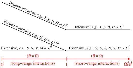
Figure 3. Schematic representation of the different scaling regimes for classical d-dimensional systems. In the case of attractive long-ranged interactions (i.e., $0\le \alpha /d\le 1$, $\alpha$ characterizing the interaction range in a potential with the form $1/r^{\alpha }$; for example, Newtonian gravitation corresponds to $(d,\alpha )=(3,1)$), we may distinguish three classes of thermodynamic variables, namely, those scaling with $L^{\theta }$, named pseudo-intensive (L is a characteristic linear length, $\theta$ is a system-dependent parameter), those scaling with $L^{d+\theta }$ with $\theta =d-\alpha$, the pseudo-extensive ones (the energies), and those scaling with $L^d$ (which are always extensive). In the case of short-ranged interactions (i.e., $\alpha >d$), we have $\theta =0$ and the energies recover their standard $L^d$ extensive scaling, falling within the same class of S, N, V, M, etc., whereas the previous pseudo-intensive variables become truly intensive ones (independent of L); this is the region, with only two classes of variables that is covered by the traditional textbooks of thermodynamics. From [26,30,33,47,48,49].

Let us also emphasize that, consistently, (i) the ratio of any two pseudo-intensive variables ($T,p,\mu ,H,\cdots$), e.g., $p/T$, is intensive in all cases; (ii) the ratio of any pseudo-extensive variable $(G,F,U)$ with any pseudo-intensive variable, e.g., $U/T$, is extensive in all cases. A most important implication of these facts is that, in expressions such as $e_q^{-{\beta }_q{\mathcal{H}}_N}$ where ${\mathcal{H}}_N$ is the N-body Hamiltonian (see Section 2.6 here below), the argument ${\beta }_q{\mathcal{H}}_N$ is extensive in all cases. This plays a crucial role in the possible q-generalization of what is currently referred to as the Large Deviation Theory. Indeed, the extensivity of ${\beta }_q{\mathcal{H}}_N$ appears to mirror, in all cases, the extensivity of the total entropy involved in $r_{q}N$, $r_q$ being the ratio function, possibly always related to some relative nonadditive entropy per particle.

2.5. Classification of Entropic Functionals

There is no unique classification or taxonomy of entropic functionals. A few facts must nevertheless be emphasized. First, the Boltzmann–Gibbs entropy $S_{BG}$ and the Renyi entropy $S_q^R$ are the unique to be additive. All the others that are present in the literature are nonadditive.

Second, it is interesting to refer to trace-form entropies S since they are the only ones that can be expressed as $S=k⟨\sigma ⟩$, where $\sigma$ is the previously introduced intuitive surprise function, which vanishes in the case of certainty and diverges in the case of vanishing probability of occurrence.

Third, we consider now another property for a dimensionless entropic form $S\left(\left\{p_i\right\}\right)/k$, namely composability. An entropy is said composable [50,51] (see also [26,52,53]) if the entropy $S(A+B)/k$ corresponding to a system composed of two probabilistically independent subsystems A and B can be expressed in the form

$$\frac{S(A+B)}{k}=F\left(\frac{S\left(A\right)}{k},\frac{S\left(B\right)}{k};\left\{\eta \right\}\right),$$

(24)

where $F(x,y;\{\eta \left\}\right)$ is a smooth function of $(x,y)$ which depends on a (typically small) set of universal indices $\left\{\eta \right\}$ defined in such a way that $F(x,y;\{0\left\}\right)=x+y$ (additivity), and which satisfies $F(x,0;\{\eta \left\}\right)=x$ (null-composability), $F(x,y;\{\eta \left\}\right)=F(y,x;\{\eta \left\}\right)$ (symmetry), $F(x,F(y,z;\left\{\eta \right\});\{\eta \left\}\right)=F\left(F\right(x,y;\left\{\eta \right\}),z;\{\eta \left\}\right)$ (associativity). This associativity appears to be consistent, for thermodynamical systems, with the $0th$ Principle of Thermodynamics. In other words, the whole concept of composability is constructed upon the requirement that the entropy of $(A+B)$ does not depend on the microscopic configurations of A and of B. Equivalently, we are able to macroscopically calculate the entropy of the composed system without any need of entering into the knowledge of the microscopic states of the subsystems. This property appears to be a natural one for an entropic form if we desire to use it as a basis for a statistical mechanics which would naturally connect to thermodynamics. The entropy $S_{BG}$ is composable since it satisfies Equation (24). More precisely, we have $F_{BG}(x,y)=x+y$. Being $S_{BG}$ nonparametric, no index exists in $F_{BG}$.

Fourth, most but not all entropies available in the literature recover $S_{BG}$ as a particular case.

Let us finally mention that the Enciso–Tempesta theorem [54] establishes that the (generically nonadditive) entropy $S_q$ is the only one which simultaneously is trace-form, composable, and contains $S_{BG}$ as a particular case. See Figure 4. For further properties of $S_q$ and other entropies, the reader might refer to [55]. In addition, a quite general structure, usually referred to as the $\Phi$-entropy, and its mathematical properties are available at [56].

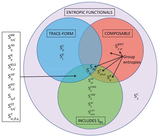
Figure 4. It has been proved [54] that $S_q$ is the unique entropic form which simultaneously is trace-form, composable, and recovers $S_{BG}$ as a particular instance. $S_q$ (hence $S_{BG}$), the Renyi entropy $S_q^R$ [14], the Tempesta $(a,b,\alpha )$-entropy $S_{a,b,\alpha }^T$ (Equation (9.1) in [57]), the Jensen–Pazuki–Pruessner–Tempesta entropy $S_{\gamma ,\alpha }^{JPPT}$ [58] and many others belong to the class of group entropies and are therefore composable. To facilitate the identification, we are here using the following notations: Sharma–Mittal entropy $S_{q,r}^{SM}$ [20,21,22], Landsberg–Vedral–Rajagopal–Abe entropy $S_q^{LVRA}$ [59,60,61], Tsallis–Mendes–Plastino entropy $S_q^{TMP}$, Arimoto entropy $S_q^{Ar}$ [62], Curado–Tempesta–Tsallis entropy $S_{a,b,r}^{CTT}$ [63], Borges–Roditi entropy $S_{q,q^{\prime }}^{BR}$ [64], Abe entropy $S_q^{Ab}$ [65], Kaniadakis entropy $S_{\kappa }^K$ [66,67,68], Kaniadakis–Lissia–Scarfone entropy $S_{\kappa ,r}^{KLS}$ [69], Anteneodo–Plastino entropy $S_{\eta }^{AP}$ [70], Hanel–Thurner entropy $S_{c,d}^{HT}$ [71,72], $S_{q,\delta }$ [30], Schwammle–Tsallis entropy $S_{q,q^{\prime }}^{ST}$ [73], the Tempesta $(\alpha ,\beta ,q)$-entropy $S_{\alpha ,\beta ,q}^T$ [74], the Curado b-entropy $S_b^C$ [75,76], the Curado $\lambda$-entropy $S_{\lambda }^C$ [33], and the exponential c-entropy $S_c^E$ [77]; one more exponential form is, in fact, available in the literature, namely the Pal and Pal non-composable trace-form entropy $S^{PP}$ [78]. The entropic form $S_{\lambda }^C$ is a rare case which does not include $S_{BG}$ and is neither trace-form nor composable. From [33].

2.6. Boltzmann–Gibbs and Nonextensive Statistical Mechanics

2.6.1. Boltzmann–Gibbs Statistical Mechanics

In the canonical form of BG statistics (for a not necessarily large system in thermal equilibrium with a much larger thermostat at temperature T), the entropy $S_{BG}\left(\left\{p_i\right\}\right)$ is maximized with the constraints

$$\sum _{i=1}^W{p}_i=1$$

(25)

and

$$\sum _{i=1}^W{p}_i{E}_i=U_{BG},$$

(26)

where $E_i$ is the energy corresponding to the i-th state of the entire N-body system. The thermal equilibrium distribution which comes out is given by the celebrated BG exponential weight

$$p_i=\frac{e^{-\beta E_i}}{Z_{BG}\left(\beta \right)}(\beta =1/kT),$$

(27)

with the partition function defined as

$$Z_{BG}\left(\beta \right)\equiv \sum _{i=1}^W{e}^{-\beta E_i}.$$

(28)

Important relations that are straightforwardly implied by this result include the Clausius relation

$$\frac{1}{T}=\frac{\partial S_{BG}}{\partial U_{BG}},$$

(29)

the Helmholtz free energy

$$F_{BG}\left(\beta \right)\equiv U_{BG}-T{S}_{BG}=-(1/\beta )ln{Z}_{BG}\left(\beta \right),$$

(30)

the internal energy

$$U_{BG}\left(\beta \right)=-\frac{\partial ln{Z}_{BG}\left(\beta \right)}{\partial \beta },$$

(31)

and the specific heat

$$C_{BG}\equiv T\frac{\partial S_{BG}}{\partial T}=\frac{\partial U_{BG}}{\partial T}=-T\frac{{\partial }^2{F}_{BG}\left(\beta \right)}{\partial T^2}\ge 0.$$

(32)

All these expressions are consistent with the Legendre structure of thermodynamics. In addition, they enable, whenever mathematically tractable, first-principle calculations of quantities, such as equation of states, specific heat, magnetic susceptibility, and others, which are simply inaccessible to thermodynamics alone [79,80].

2.6.2. q-Generalization of the Boltzmann–Gibbs Theory

If we adopt an entropic functional differing from $S_{BG}$ but containing it as a particular instance, we can formally generalize the BG theory. When we adopt as basis the nonadditive entropy $S_q$, such a generalization is usually referred to as nonextensive statistical mechanics [25,26], as mentioned earlier. This generalization can be outlined through various, basically equivalent [81,82], paths. We follow here the version developed in [83]. We optimize $S_q$ (maximize for $q>0$ and minimize for $q<0$) with the constraints (25) and

$$\frac{{\sum }_{i=1}^W{p}_i^q{E}_i}{{\sum }_{i=1}^W{p}_i^q}=U_q,$$

(33)

where we impose, for reasons that are analyzed in [84], the average of $E_i$ by using the escort distribution $p_i^q/{\sum }_{i=1}^W{p}_i^q$, instead of simply $p_i$. This procedure yields the following q-generalized results:

$$p_i=\frac{e_q^{-{\beta }_q(E_i-U_q)}}{{\overline{Z}}_q\left({\beta }_q\right)},$$

(34)

with

$${\overline{Z}}_q\left({\beta }_q\right)\equiv \sum _{i=1}^W{e}_q^{-{\beta }_q(E_i-U_q)},$$

(35)

and

$${\beta }_q=\frac{\beta }{{\sum }_{i=1}^W{p}_i^q},$$

(36)

$\beta \equiv 1/kT$ being the Lagrange parameter. The q-exponential function is defined as $e_q^z\equiv {[1+(1-q)z]}^{\frac{1}{1-q}}$ if $[1+(1-q\left)z\right]>0$ and zero otherwise, with $e_1^z=e^z$. It is the inverse of the q-logarithmic function, i.e., $e_q^{{ln}_{q}z}={ln}_q{e}_q^z=z$.

We can rewrite Equation (34) as follows:

$$p_i=\frac{e_q^{-{\beta }_q^{\prime }{E}_i}}{Z_q^{\prime }\left({\beta }_q^{\prime }\right)},$$

(37)

with

$${\beta }_q^{\prime }\equiv \frac{{\beta }_q}{1+(1-q){\beta }_q{U}_q},$$

(38)

and

$$Z_q^{\prime }\left({\beta }_q^{\prime }\right)\equiv \sum _{i=1}^W{e}_q^{-{\beta }_q^{\prime }{E}_i}.$$

(39)

In addition, it can be proved that

$$\frac{1}{T}=\frac{\partial S_q}{\partial U_q},$$

(40)

$$F_q\left(\beta \right)\equiv U_q\left(\beta \right)-T{S}_q\left(\beta \right)=-(1/\beta ){ln}_q{Z}_q\left(\beta \right),$$

(41)

with

$${ln}_q{Z}_q={ln}_q{\overline{Z}}_q-\beta U_q,$$

(42)

and

$$U_q\left(\beta \right)=-\frac{\partial {ln}_q{Z}_q\left(\beta \right)}{\partial \beta },$$

(43)

and

$$C_q\equiv T\frac{\partial S_q}{\partial T}=\frac{\partial U_q}{\partial T}=-T\frac{{\partial }^2{F}_q\left(T\right)}{\partial T^2}.$$

(44)

As before, these expressions are consistent with the Legendre structure of thermodynamics. In addition, as for the BG theory (here recovered as the $q=1$ particular case), they enable, whenever mathematically tractable, first-principle calculations of quantities, such as equation of states, specific heat, magnetic susceptibility, and others, which are simply inaccessible to thermodynamics alone. Some analytical calculations of this type, focusing on overdamped many-body systems, are available in [85,86,87,88,89,90,91,92,93].

As a final remark, it is worthy to emphasize that the BG entropy and associated statistical mechanics appear to be sufficient but not necessary for the validity of classical thermodynamics and the Einstein likelihood principle, see [94].

3. Results and Applications

The ubiquitous applications of $S_{BG}$ and associated statistical mechanics are not reviewed here since a vast literature profusely describes them during the last 150 years (see, e.g., [80] and references therein). We shall here restrict our focus onto some typical applications of non-BG entropies, mainly those of the popular $S_q$, in physics and beyond, thus illustrating this vast and intensively developing field.

3.1. In Physics

3.1.1. Nonlinear Dynamical Systems

Nonlinear dynamics has various direct connections with the time evolution of the entropy of a system and its consequences. There are, in this respect, two important classes of chaotic behavior, namely strong chaos, characterized by exponential sensitivity to the initial conditions (referred to, for classical systems, as having a positive maximal Lyapunov exponent) and weak chaos, characterized by subexponential (frequently power-law) sensitivity to the initial conditions (referred to, for classical systems, as having a vanishing maximal Lyapunov exponent). We focus here on two important issues: (i) the time evolution of the entropy while exploring the system phase-space, and (ii) the Central Limit Theorem attractor in the space of distributions when averaging along time a single coordinate of the system.

(i) Let us illustrate the first issue with a paradigmatic dissipative system, namely the logistic map $x_{t+1}=1-a{x}_t^2(x_t\in [-1,1];a\in [0,2];t=0,1,2,\cdots )$. For $a=2$, the system is strongly chaotic since the sensitivity to the initial conditions satisfies $\xi \equiv {lim}_{\Delta x\left(0\right)\to 0}\frac{\Delta x\left(t\right)}{\Delta x\left(0\right)}=e^{\lambda t}$ with a Lyapunov exponent $\lambda =ln2>0$. Consistently, if we start at $t=0$ from a set of M initial conditions in an arbitrarily chosen single window within W of them equally partitioning the interval $[-1,1]$, we obtain the entropy production per unit time

$$K_{BG}\equiv \underset{t\to \infty }{lim}\underset{W\to \infty }{lim}\underset{M\to \infty }{lim}\frac{S_{BG}\left(t\right)/k}{t}=\lambda >0,$$

(45)

thus verifying the Pesin identity. We also verify that $K_q\equiv {lim}_{t\to \infty }{lim}_{W\to \infty }{lim}_{M\to \infty }\frac{S_q\left(t\right)/k}{t}$ vanishes if $q>1$ and diverges if $q<1$. In other words, $q=1$ is the unique value of the index for which $S_q\left(t\right)$ asymptotically increases linearly with time. See Figure 5.

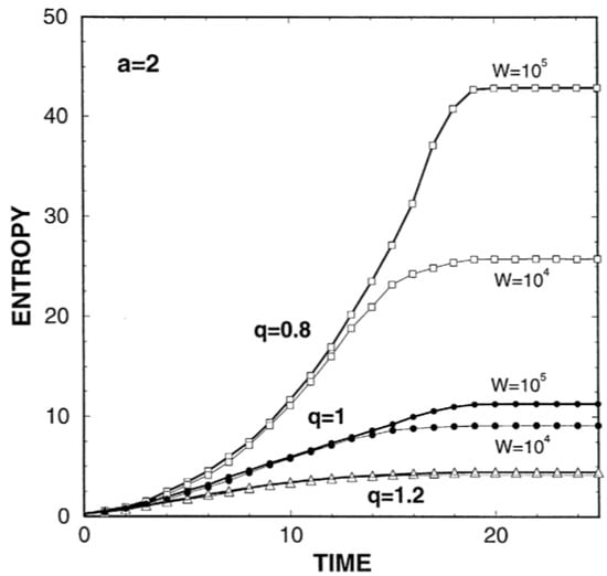
Figure 5. Time evolution of $S_q$ for $a=2$. The interval $[-1,1]$ is partitioned into W equal cells. The initial distribution consists of $M={10}^6$ points placed at random inside a randomly picked cell. We indicate three typical values of q and the two cases $W={10}^4$ and $W={10}^5$. Results are averages over 100 runs. From [95].

If we do the same operations at the edge of chaos, more precisely at the Feigenbaum (or Feigenbaum–Coullet–Tresser) point $a=a_c\equiv 1.40115518909\cdots$, which corresponds to a vanishing Lyapunov exponent $\lambda$ (i.e., weak chaos), we verify that $\xi =e_{q_{sensitivity}}^{{\lambda }_{q_{sensitivity}}t}$ with $q_{sensitivity}=0.244487701341282066198\cdots$ and ${\lambda }_{q_{sensitivity}}=1/(1-q_{sensitivity})$. It follows that, for $t\to \infty$, $\xi$ diverges subexponentially, more precisely, a power-law $\xi \propto t^{1/(1-q_{sensitivity})}$. Moreover, it can be shown that $\frac{1}{1-q_{sensitivity}}=\frac{1}{{\alpha }_{min}}-\frac{1}{{\alpha }_{max}}=\frac{ln{\alpha }_F}{ln2}$, where ${\alpha }_F$ is the so-called Feigenbaum universal constant, the multifractal function $f\left(\alpha \right)$ being concave, defined in the interval $[{\alpha }_{min},{\alpha }_{max}]$ with $f\left({\alpha }_{min}\right)=f\left({\alpha }_{max}\right)=0$. Analogously to the BG case, we verify a q-generalized Pesin identity $K_{q_{entropy}}={\lambda }_{q_{entropy}}$ with $q_{entropy}=q_{sensitivity}$ and ${\lambda }_{q_{entropy}}={\lambda }_{q_{sensitivity}}$. See Figure 6. Consistently, we have that $K_q$ vanishes for $q>q_{entropy}$ and diverges for $q<q_{entropy}$.

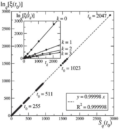
Figure 6. Numerical confirmation (full circles) of the q-generalized Pesin-like identity $K_q^{\left(k\right)}={\lambda }_q^{\left(k\right)}$ at the logistic-map edge of chaos. On the ordinate, we plot the q-logarithm of ${\xi }_{t_k}$ (equal to ${\lambda }_q^{\left(k\right)}t$), and, on the abscissa, $S_q$ (equal to $K_q^{\left(q\right)}t$), both for $q=0.2445...$ The dashed line is a linear fit. Inset: The full lines are from the analytic result. From [96].

(ii) Let us illustrate now the second issue, still with the same logistic map. Along the Central Limit Theorem line, we may define $y\equiv {\sum }_{t=1}^T{x}_t$. For $a=2$, we have that, after proper scaling and centering, the distribution $P\left(y\right)$ is given by a Gaussian, according to the classical Central Limit Theorem, whereas, for $a=a_c$, it is given by a $q_{attractor}$-Gaussian with $q_{attractor}=1.66\pm 0.04$, see Figure 7. Incidentally, we verify for the logistic map at the Feigenbaum point (edge of chaos) that $q_{sensitivity}=q_{entropy}\ne q_{attractor}$. This is a generic tendency of many non-Boltzmann–Gibbs systems. More precisely, there might be not only one but various indices q differing from unity which are associated to various properties of the same system under specific classes of initial or boundary conditions. However, similarly to the critical exponents within the standard theory of phase transitions, relatively simple relations are expected to exist among these various q-values.

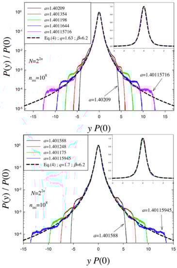
Figure 7. Data collapse of probability density functions (in log-linear plots) for $T=2^{2n}$, where $2n$ is an odd number (top) or an even number (bottom). As n increases, good fits with $q_{attractor}$-Gaussian $\propto e_{q_{attractor}}^{-\beta y^2}$ (with $(q_{attractor},\beta )=(1.63,6.2)$ (top), and $(q_{stat},\beta )=(1.70,6.2)$ (bottom)) are obtained for increasingly large regions. Insets: Linear-linear plots of the data for a better visualization of the central part. From [97].

Let us further illustrate the second issue, now with a paradigmatic conservative system, namely the standard map introduced by Chirikov in 1979:

$$\begin{array}{ccc}\hfill p_{i+1}& =& p_i-Ksin{x}_i\left(mod2\pi \right)(K\ge 0)\hfill \\ \hfill x_{i+1}& =& x_i+p_{i+1}\left(mod2\pi \right)\hfill \end{array}$$

(46)

Typical phase portraits are shown in Figure 8. Each $(x,p)$ point yields a Lyapunov exponent ${\lambda }^{\left(1\right)}=-{\lambda }^{\left(2\right)}\ge 0$, see Figure 9. Next, along the Central Limit Theorem lines, we define the following quantity

$$\overline{y}\equiv \sum _{i=1}^T(x_i^{\left(j\right)}-⟨x⟩),$$

(47)

with

$$⟨x⟩\equiv \frac{1}{M}\frac{1}{T}\sum _{j=1}^M\sum _{i=1}^T{x}_i^{\left(j\right)},$$

(48)

where $M>>1$ (typically $M\ge {10}^7$) is the number of initial conditions and $T>>1$ (typically $T\ge 2^{23}\simeq {10}^7$) is the number of iterations for each of those M initial conditions. Finally, by constructing the histogram for $\overline{y}$, we obtain the results indicated in Figure 10 and Figure 11. The limiting $K=0$ case (hence a linear map, though with a highly nontrivial set of stable orbits) has been revisited, along the same lines, with higher precision [98] and the value $q_{attract}\simeq 1.935$ has been re-obtained. Nevertheless, since some numerical error naturally persists, an analytical effort has been accomplished [99] and the exact value turns out to be $q_{attract}=2$.

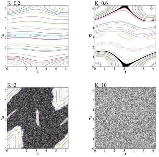
Figure 8. Phase portrait of the standard map for representative values of K. In each case, black dots represent the region of chaotic sea in the available phase space and all other colors represent different stability islands. From [100].

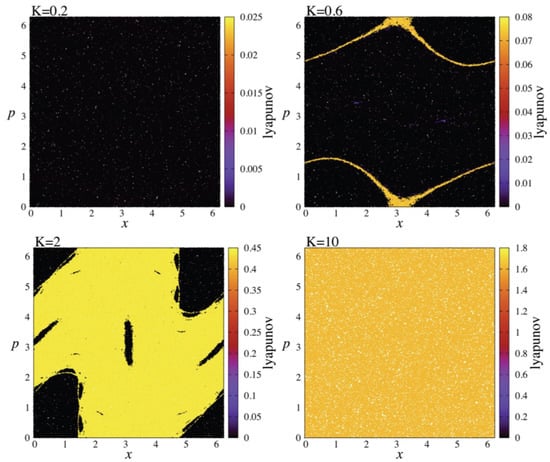
Figure 9. Lyapunov exponent results of the phase portrait of the standard map. The same representative K values are used. For each case, Lyapunov exponents are calculated for 200,000 initial conditions. In the calculation, each initial condition is iterated 107 times. From [100].

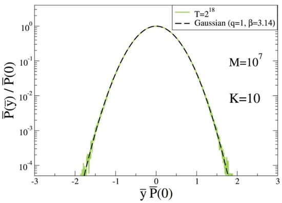
Figure 10. Normalized probability distribution function for $K=10$ with $T=2^{18}$. From [100].

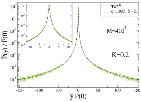
Figure 11. Normalized probability distribution function for $K=0.2$ with $T=2^{22}$. From [100].

3.1.2. First-Principle Calculation of q for a Quantum Hamiltonian System

The calculation of q from first principles is mathematically tractable in some cases. One such example is the quantum phase transition at $T=0$ for the $d=1$ first-neighbor Ising ferromagnet in the presence of a transverse magnetic field, and similar quantum systems characterized by a central charge $c\ge 0$. A subsystem of linear size L of an infinitely long such chain satisfies $S_{BG}\left(L\right)\propto lnL$, which is nonextensive and violates therefore the Legendre structure of thermodynamics. It turns out, however, that a value of q, noted $q_{entropy}$, exists such that $S_{q_{entropy}}\left(L\right)\propto L$, thus satisfying thermodynamics. Its value is given [101] by

$$q_{entropy}=\frac{\sqrt{9+c^2}-3}{c},$$

(49)

which is depicted in Figure 12.

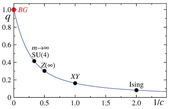
Figure 12. The index $q_{entropy}$ as a function of the inverse central charge $1/c$. The universality classes of some specific models are indicated, see [94]. The BG value $q_{entropy}=1$ is recovered in the $c\to \infty$ limit.

3.1.3. Long-Range Interactions

As discussed in Section 2.3, Gibbs himself dismissed [5,6,7] BG statistical mechanics whenever anomalies such as say long-range interactions make the partition function function to diverge. This means that, for $\alpha /d>1$ in the classical systems focused on in that Section, we expect the distribution of velocities to be Maxwellian (i.e., $q_{momenta}=1$), and the distribution of energies to precisely be the BG weight (i.e., $q_{energy}=1$). In contrast, models, such as the d-dimensional $\alpha$-XY [36] and $\alpha$-Heisenberg [37,38,39] ferromagnets, as well as the $\alpha$-Fermi–Pasta–Ulam [42,43,44] one, are numerically shown to violate the BG theory and exhibit q-statistics instead. This is illustrated for the $\alpha$-XY ferromagnet in Figure 13 and Figure 14. For $\alpha /d=0.9$, we obtain $q_{momenta}\simeq 1.6$ and $q_{energy}\simeq 1.3$, whereas, for $\alpha /d=2$, we verify that $q_{momenta}=1$.

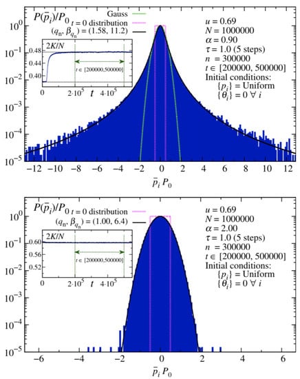
Figure 13. A typical single-initial-condition one-momentum distribution $P\left(p\right)$ for $N={10}^6$, $u=0.69$, $\tau =1$ (corresponding to 5 molecular-dynamics steps), calculated in the region $[t_{min};t_{max}]=[200,000;500,000]$ for $\alpha =0.9$ (top plot), and $\alpha =2.0$ (bottom plot). The upper temperature indicated in the $\alpha =0.9$ inset coincides with that analytically calculated within BG statistical mechanics, namely $T_{kin}\equiv 2K\left(t\right)/N\simeq 0.475$. The horizontal line of the $\alpha =2.0$ inset corresponds to the numerically calculated time average; indeed, analytical solutions are only available for $\alpha <1$ and in the $\alpha \to \infty$ limit. The continuous curves correspond to $P\left(\tilde{p}\right)/P_0=e_{q_n}^{-{\beta }_{q_n}^{\left(P_0\right)}\left[\tilde{p}{P}_0\right){]}^2/2}$ with $(q_n,{\beta }_{q_n}^{\left(P_0\right)})=(1.58,11.2)$ for $\alpha =0.9$ and (1.0,6.4) for $\alpha =2.0$. Notice that, for $\alpha =0.9$, $1/{\beta }_{q_n}^{\left(P_0\right)}\ne T$. Each distribution has been rescaled with its own $P_0$. From [102].

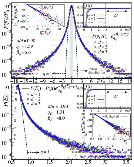
Figure 14. Distributions of the time-averages of the momenta ${\overline{p}}_i$ and of the energies ${\overline{E}}_i$ (with $\tau =1$) for $\alpha /d=0.9$, in $d=1$, 2 and 3 dimensions. The simulations were done for the energy per particle $u=0.69$ and total number of rotators $N={10}^6$. Top: Distribution $P\left({\overline{p}}_i\right)$ is shown ($P_0\equiv P({\overline{p}}_i=0)$), the full line being a q-Gaussian with $q_p=1.59$ and ${\beta }_p=5.6$, and the dashed line being a Gaussian $(q=1)$. The left inset shows the same data in a q-logarithm versus squared-momentum representation; a straight line is obtained as expected (since ${ln}_q\left(e_q^x\right)=x$). Bottom: The full line represents the q-exponential $P\left({\overline{E}}_i\right)=P\left(\mu \right){exp}_{q_E}[-{\beta }_E({\overline{E}}_i-\mu )]$, with $q_E=1.31$ (${\beta }_E=48.0$, $\mu =0.69$, and $P\left(\mu \right)=12$); the corresponding exponential (dashed line) is also shown for comparison. Since the density of states is necessary to reproduce the entire range of data, a chemical potential $\mu$ was introduced in the fitting. The bottom inset shows a straight line by using the q-logarithm in the ordinate. The kinetic temperature $T\left(t\right)\equiv 2K\left(t\right)/N$ and time window $\Delta t$, along which the time averages were calculated, coincide in both cases (shown as insets). One notices that, in all plots, the collapse of all dimensions occurs with nearly the same value of q. From [103].

3.1.4. Overdamped Many-Body Systems

In various overdamped classical d-dimensional many-body systems including short-range repulsive interactions, it has been possible to analytically calculate and numerically verify the validity of q-statistics, focusing on space and velocity distributions, equations of states, Carnot cycle, H-theorem and the 0-$th$ principle of thermodynamics [85,86,87,88,89,90,91,92,93,104]. For example, for repulsive interactions proportional to $1/r^{\alpha }$, it is proved [104] that $q_{position}=1-\alpha /d<1$, which, in the limit $\alpha /d\to 0$, recovers the result $q_{position}=q_{momenta}=0$ [85,86,87]. This class of systems constitute a rare case where nearly all thermostatistical quantities can be analytically calculated, thus verifying q-statistics.

3.1.5. Low Energy Physics

Several validations of q-statistics are available in the literature for low-energy systems. Two of them are selected here as illustrations: cold atoms and granular matter.

In 2003, Lutz suggested [105] that the velocity distribution of cold atoms in dissipative optical lattices should be a q-Gaussian with $q=1+44E_R/U_0$, $E_R$ and $U_0$ being parameters of the lattice potential. The Lutz prediction was computationally and experimentally verified in 2006 [106,107], see Figure 15.

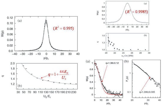
Figure 15. Quantum Monte Carlo verification (left panels) [(a) Analytic and numerical distributions; (b) Analytical and numerical functions $q(U_0/E_r)$], and laboratory verification with $C_s$ atoms (right panels) [(Top a) Analytical and experimental distributions; (Bottom b) Experimental frequency dependence of q; (Left a) Linear-linear representation of the experimental distribution of momenta, the black curve corresponding to the present q-Gaussian, the red curve corresponding to a Maxwellian distribution; (Right b) The same in log-log representation.] of the 2003 Lutz prediction. From [106].

Another experimental validation of q-statistics was performed for granular matter. In 1996, the scaling law $\alpha =2/(3-q)$ was predicted [108], $\alpha$ being defined from the anomalous diffusion scaling $x^2\sim t^{\alpha }$, and q corresponding to the index of the q-Gaussian solution of the nonlinear Fokker–Planck equation introduced by Plastino and Plastino [109]. This prediction was verified within $\pm 2\%$ error in 2015 [110], see Figure 16, Figure 17 and Figure 18.

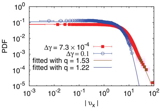
Figure 16. Probability density functions of the horizontal components of the randomly fluctuating displacements tracked during two typical increments of shear strain ($\Delta \gamma =7.3\times {10}^{-4}$ and $\Delta \gamma ={10}^{-1}$). The scatters correspond to experimental data, and the solid lines correspond to q-Gaussian fittings. From [110].

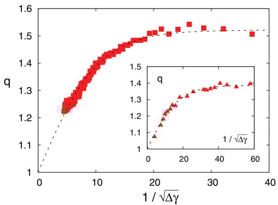
Figure 17. Evolution of the measured value q as a function of the squared inverse of the strain increment for both the experiments and simulations. The dashed line corresponds to a regression using the function $q(1/\sqrt{\Delta \gamma })=1+atanh(b/\sqrt{\Delta \gamma })$, with $(a,b)=(0.521,0.096)$. Inset: The same plot for data from a simulation that highlights the limit $q=1$ when $\Delta \gamma \to \infty$. The fitted parameters for simulations were $(a,b)=(0.387,0.057)$. From [110].

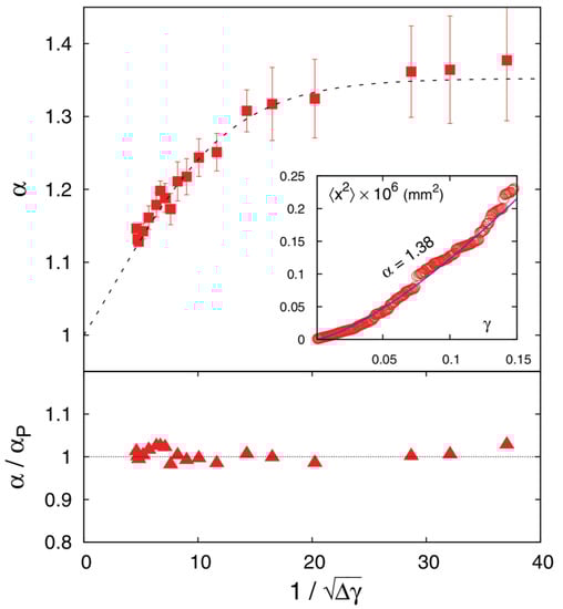
Figure 18. Verification of the scaling law $\alpha =2/(3-q)$ [108] for several regimes of diffusion. Top: Evolution of the measured diffusion exponent $\alpha$ as a function of $1/\sqrt{\Delta \gamma }$; the dashed line is a direct application of the scaling law from the fit of the values shown in Figure 17, $\alpha (1/\sqrt{\Delta \gamma })=2/[3-q(1/\sqrt{\Delta \gamma })]$. Inset: A typical diffusion curve showing the mean square displacement fluctuations $⟨x^2⟩$ as a function of the shear strain $\gamma$; this allows the assessment of the diffusion exponent $\alpha \equiv \mu$ for each strain window tested. In the case shown, it corresponds to the smallest strain window, the rightmost point in the curve in the main panel. Note that for a constant strain rate, $\gamma$ is proportional to time. Bottom: Measure of the deviation of the data relative to the scaling law prediction ${\alpha }_P=2/(3-q)$, as a function of $1/\sqrt{\Delta \gamma }$, showing a remarkable agreement of the order of $\pm 2\%$. From [110].

3.1.6. High Energy Physics

Many validations of q-statistics are available in the literature for high-energy systems. Two of them are selected here as illustrations: high-energy collisions experiments at LHC/CERN [111] and AMS-02 observations of matter and anti-matter [112], see Figure 19 and Figure 20, respectively.

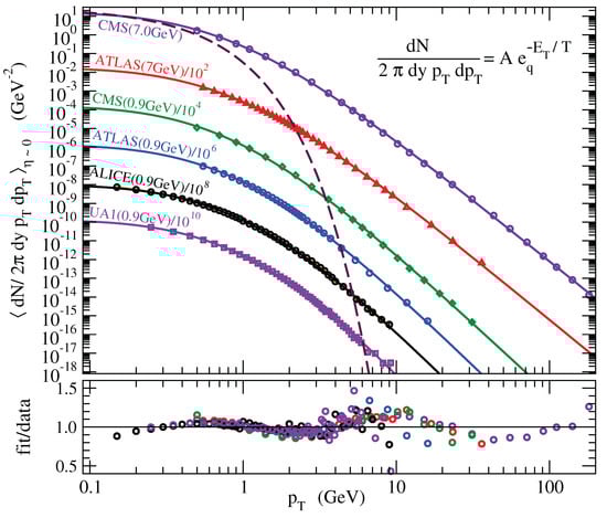
Figure 19. Experimental transverse momentum distribution of hadrons in $pp$ collisions at central rapidity y compared with theoretical q-exponentials with $q\simeq 1.13\pm 0.02$ and $T\simeq (0.14\pm 0.01)GeV$. The corresponding Boltzmann–Gibbs (purely exponential) fit is illustrated as the dashed curve. The data and the analytical curves have been divided by a constant factor as indicated, for a better visualization. The ratios data/fit are shown at the bottom, where a nearly log-periodic behavior is observed on top of the q-exponential one. See [111] for details.

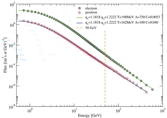
Figure 20. The measured AMS-02 data are very well fitted by linear combination of escort and non-escort distributions (solid lines); $q_1=13/11$ and $q_2=1/(2-q_1)=11/9$. From [112].

3.2. Beyond Physics

3.2.1. Mathematics

The product $xy$ of two real numbers has been conveniently generalized as the following q-product [113,114]:

$$x{\otimes }_{q}y\equiv e_q^{{ln}_{q}x+{ln}_{q}y}={\left[x^{1-q}+y^{1-q}-1\right]}_{+}^{\frac{1}{1-q}}(x\ge 0,y\ge 0),$$

(50)

where ${[\cdots ]}_{+}=[\cdots ]$ if $[\cdots ]>0$ and vanishes otherwise. Let us list some of its main properties:

(i) It recovers the standard product as the $q=1$ particular instance, i.e.,

$$x{\otimes }_{1}y=xy;$$

(51)

(ii) It is commutative, i.e.,

$$x{\otimes }_{q}y=y{\otimes }_{q}x;$$

(52)

(iii) It is additive under q-logarithm, i.e.,

$${ln}_q\left(x{\otimes }_{q}y\right)={ln}_{q}x+{ln}_{q}y,$$

(53)

whereas we remind that

$${ln}_q\left(xy\right)={ln}_{q}x+{ln}_{q}y+(1-q)\left({ln}_{q}x\right)\left({ln}_{q}y\right).$$

(54)

Consistently,

$$e_q^x{\otimes }_q{e}_q^y=e_q^{x+y},$$

(55)

whereas

$$e_q^x{e}_q^y=e_q^{x+y+(1-q)xy};$$

(56)

(iv) It is associative, i.e.,

$$x{\otimes }_q\left(y{\otimes }_{q}z\right)=\left(x{\otimes }_{q}y\right){\otimes }_{q}z=x{\otimes }_{q}y{\otimes }_{q}z={(x^{1-q}+y^{1-q}+z^{1-q}-2)}^{1/(1-q)};$$

(57)

(v) It admits unity, i.e.,

$$x{\otimes }_{q}1=x;$$

(58)

(vi) It admits zero under certain conditions, more precisely,

$$\begin{array}{c}\hfill x{\otimes }_{q}0=\left\{\begin{array}{c}0\mathrm{if}\left(q\ge 1\mathrm{and}x\ge 0\right)\mathrm{or}\mathrm{if}\left(q<1\mathrm{and}0\le x\le 1\right),\\ \\ {\left(x^{1-q}-1\right)}^{\frac{1}{1-q}}\mathrm{if}q<1\mathrm{and}x>1;\end{array}\right.\end{array}$$

(59)

On the basis of this product, it is possible to generalize, for $q\ge 1$, the Fourier-Transform of a nonnegative function $f\left(x\right)$ as follows: [115,116]:

$$F_q\left[f\right]\left(\xi \right)\equiv \int dx{e}_q^{i\xi x}{\otimes }_{q}f\left(x\right)F_q\left[f\right]\left(\xi \right)={\int }_{-\infty }^{\infty }dx{e}_q^{i\xi x{\left[f\left(x\right)\right]}^{q-1}}f\left(x\right).$$

(60)

It is clear that this transformation is, for $q\ne 1$, nonlinear. Indeed, if we do $f\left(x\right)\to \lambda f\left(x\right)$, $\lambda$ being any constant, we straightforwardly verify that $F_q\left[\lambda f\right]\left(\xi \right)\ne \lambda F_q\left[f\right]\left(\xi \right)$. This generalization of the standard Fourier transform $F_1\left[f\right]\left(\xi \right)$ was introduced in order to have a remarkable property: it transforms q-Gaussians into q-Gaussians. Indeed, the following equality can be easily verified:

$$F_q\left[B_q\sqrt{\beta }{e}_q^{-\beta x^2}\right]\left(\xi \right)=e_{q_1}^{-{\beta }_1{\xi }^2},$$

(61)

where

$$(q_1,{\beta }_1)=\left(\frac{1+q}{3-q},\frac{3-q}{8{\beta }^{2-q}{B}_q^{2(q-1)}}\right)(1\le q<2),$$

(62)

$B_q$ being an appropriate normalizing quantity. Within this frame, and others as well, the Central Limit Theorem has been generalized [115], showing that, while averaging a large number of random variables within a wide class of nonlocal correlations (yet only partially explored), q-Gaussians emerge as attractors in the space of distributions. This provides an epistemological basis for understanding why are there so many q-Gaussians (and consistently so many q-exponentials) in nature. Further details and proofs can be found in [117].

Another relevant line of mathematical research concerns the relations of various sets of q-indices (e.g., q-triplets) that frequently appear in complex systems [118,119].

3.2.2. Chemistry

Among the many chemical applications available in the literature, we select here a rather intriguing one concerning Mendeleev’s Table. The free atom ground-state energy (as calculated by a performant ab initio Hartree–Fock method) of all the elements approximately follows, as function of the atomic number Z, a q-exponential. Indeed, as depicted in Figure 21, from the hydrogen to the lawrencium, it is given by [120]

$$E=E_H{e}_{0.58145}^{2.4333(Z-1)}(E_H=-13.60534ev).$$

(63)

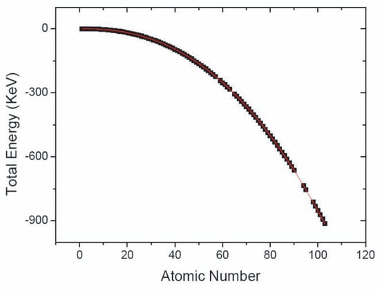
Figure 21. Ground-state energy E of the free atom as a function of the atomic number Z. The results from hydrogen to lawrencium are presented. The red line has been calculated with Equation (63). From [120].

The reason for this peculiar behavior is unknown. However, it plausibly is a consequence of the proton–electron and electron–electron long-range Coulombian interactions.

3.2.3. Economics

There are many applications of q-statistics to economics (see for instance [121,122,123]). As an illustration, we exhibit in Figure 22 the cumulative return distributions corresponding to the 100 American companies with the highest market capitalization [124].

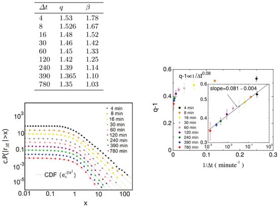
Figure 22. Left panel: Cumulative distributions of absolute normalized returns corresponding to different time scales $\Delta t$ for the 100 American companies with the highest market capitalization (points), and the fitted cumulative q-Gaussian distributions (lines). In order to better visualize the associated results, each q-Gaussian CDF and the respective experimental data have been multiplied by a positive factor $c\ne 1$. Right panel: Dependence of the index q on the time scale $\Delta t$, for the estimated q-Gaussian pdfs of normalized absolute returns in the left panel. Inset: log-log representation exhibiting a power-law dependence of the type $q-1\propto {\left(\Delta t\right)}^{-\tau }$ , with $\tau =0.081\pm 0.004$. From [124].

3.2.4. Biology and Life Sciences

Let us next focus on DNA structures as discussed in [125]. Typical results for the inter-nucleotide intervals are shown in Figure 23.

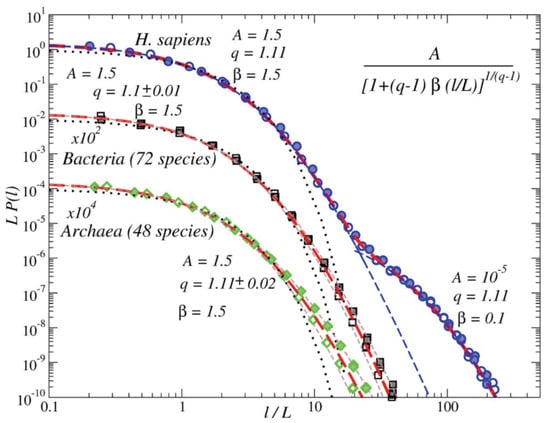
Figure 23. PDFs of the inter-nucleotide intervals A-A, T-T (open symbols); G-G, C-C (full symbols) in the DNA sequences from Homo Sapiens and Bacteria full genomes (in scaled form). Dashed lines show the best fits by a q-exponential distribution $A=1/{[1+(q-1)\beta (l/L)]}^{\frac{1}{q-1}}$. While in Bacteria the approximation by a single q-exponential with $q\sim 1.1$ and $\beta \sim 1.5$ is possible, in H. Sapiens, a sum of two q-exponentials with $q\sim 1.11$ and $\beta \sim 1.5$ and 0.1 makes the best fit. To avoid overlapping, the PDFs for Bacteria are shifted downwards by two decades. For comparison, dotted lines show corresponding exponential PDFs. From [125].

It is definitively remarkable that the value $q=1.11$ plays a universal role in so diverse biological beings. Its explanation certainly remains an open problem. Moreover, it would be undoubtedly interesting to check whether the double q-exponential behavior that is observed in Homo Sapiens is also present in other mammals.

3.2.5. Computer Sciences

The search for global minima in a cost function of many variables which simultaneously presents many local minima is a most relevant problem in all kinds of scientific and technological systems. It might be computationally very hard. One such method is the so-called Simulated Annealing (SA), also referred to as the Boltzmann machine. It consists of (i) a searching algorithm based on normal diffusion within the phase-space, (ii) an accepting algorithm based on the Boltzmann weight, and (iii) a cooling algorithm based on the monotonic decrease of temperature along time t as follows:

$$\frac{T\left(t\right)}{T\left(1\right)}=\frac{ln2}{ln(1+t)}(t=1,2,3,...),$$

(64)

where $T\left(1\right)$ is an initial high temperature imposed onto the system. A performant (both in speed and precision) q-generalization of this machine is available and usually referred to as Generalized Simulated Annealing (GSA) [126]. It generalizes the SA ingredient (i) into a $q_V$-Gaussian anomalous diffusion (typically with $q_V\ge 1$), ingredient (ii) into a $q_A$-exponential weight (typically with $q_A\le 1$), and time evolution (iii) into

$$\frac{T\left(t\right)}{T\left(1\right)}=\frac{2^{q_V-1}-1}{{(1+t)}^{q_V-1}-1}=\frac{{ln}_{q_V}(1/2)}{{ln}_{q_V}[1/(t+1)]}(t=1,2,3,...).$$

(65)

We verify that, for $q_V=q_A=1$, the Boltzmann machine is precisely recovered. The GSA algorithm is being successfully applied in physics, chemistry, computational sciences, engineering, and elsewhere when the relevant cost function presents a large amount of local minima in a multi-dimensional phase-space, by all means a very frequent case in complex systems.

3.2.6. Random Networks

Complex networks are ubiquitous in natural, artificial and social systems. Among them, many classes of either growing or non-growing, geographical or fully nonlocal, d-dimensional networks exist which exhibit asymptotic scale-invariance, typically based on various kinds of preferential attachments [127,128,129,130,131,132,133,134,135,136]. A quite general network with weighted links is introduced and numerically analyzed in [136], see Figure 24 and Figure 25.

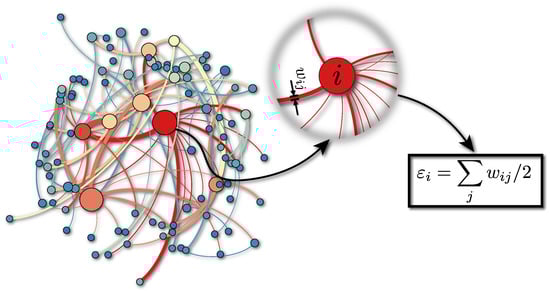
Figure 24. Sample of a network with 100 sites for the following model parameters $(d,{\alpha }_A,{\alpha }_G,\eta ,w_0)=(2,1,5,1,1)$, where ${\alpha }_A$ and ${\alpha }_G$ respectively characterize the attachment and geographical ranges; $\eta$ and $w_0$ are parameters of the distribution of widths. As illustrated for this choice of parameters, hubs (highly connected nodes) naturally emerge in the network. Each link has a specific width $w_{ij}$ and the total energy ${\epsilon }_i$ associated with the site i will be given by half of the sum over all link widths connected to the site i (see zoom of site i). From [136].

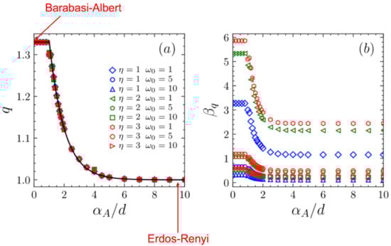
Figure 25. In all cases, the energy distribution is well fitted with the form $p_q\propto e_q^{-{\beta }_q\epsilon }$. (a) q as a function of ${\alpha }_A/d$ (black solid line); $q=4/3$ for $0\le {\alpha }_A/d\le 1$ and decreases exponentially with ${\alpha }_A/d$ for ${\alpha }_A/d>1$, down to $q_{\infty }=1$. (b) ${\beta }_q$ as a function of ${\alpha }_A/d$ for $\eta =1,2,3$ and $w_0=1,5,10$, for typical values of ${\alpha }_A/d$; ${\beta }_q$ increases with $\eta$ and decreases with $w_0$ and ${\alpha }_A/d$. From [136].

3.2.7. Image and Signal Processing

Nonadditive entropies have been profusely used in image and signal processing, in order to improve speed and clarity. Two such examples are here exhibited.

The detection of possibly pathological microcalcifications as revealed in mammograms can be sensibly improved by using q-entropy with $q\ne 1$ [137], see Figure 26.

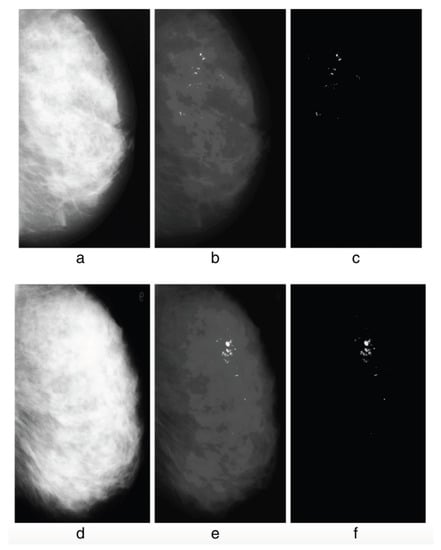
Figure 26. Without q-entropy enhancement with $q\ne 1$, detection of microcalcifications is meager: 80.21% Tps (true positives) with 8.1 Fps (false positives), whereas upon introduction of the q-entropy, the results surge to 96.55% Tps with 0.4 Fps. Detection results from the experiment: (a) mdb236, (b) output with the Mcs enhanced, (c) output with the Mcs extracted, (d) mdb216, (e) output with the Mcs enhanced, (f) output with the Mcs extracted. From [137].

The image of Computer Tomography scans revealing fibrosis due to COVID-19 can be sensibly improved by incorporating in the algorithm the q-entropy with $q=0.5$ [138], see Figure 27.

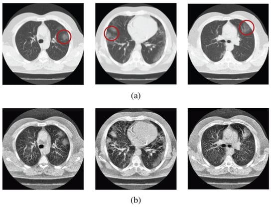
Figure 27. Sample scans from the dataset before and after enhancement showing infected lungs. (a) Original Computer Tomography scans, with red circles highlighting some regions where fibrosis can be seen; (b) enhanced Computer Tomography scans using $q=0.5$. From [138].

3.2.8. Engineering

Various engineering projects have been settled down which include nonadditive entropies and related properties. One of those projects, concerning civil engineering, is presented in Figure 28 and Figure 29. By sticking a sensible microphone onto a civil engineering material supporting variable stresses, it is possible to detect and computationally process the microfracture signals which occur. If a convenient protocol is implemented, it is possible to predict when the block will break macroscopically. This type of technique could in principle be implemented to check the structural health of buildings, bridges, monuments.

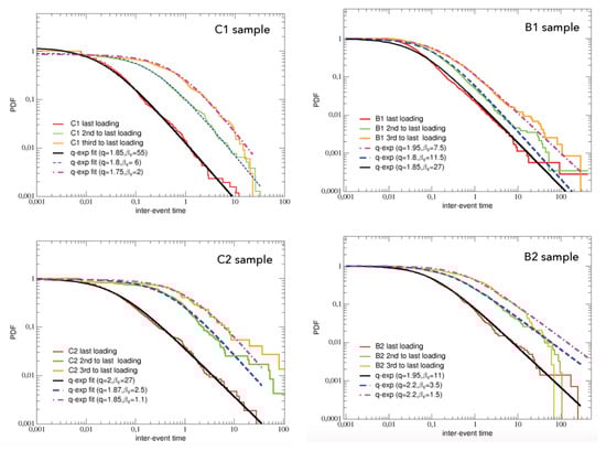
Figure 28. Cumulative pdfs of the inter-event times of acoustic emission for the last three loadings of the specimens. Left: C1, C2 (concrete) and Right: B1, B2 (basalt). The q-exponential fittings are also shown. From [139].

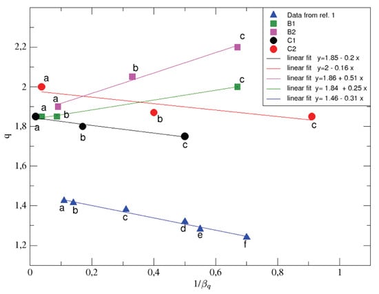
Figure 29. The values of the entropic index of the q-exponential fits, reproducing the complementary cumulative pdfs obtained from experimental data about the AE inter-event time series for both the concrete (C1, C2—full circles) and basalt (B1, B2—full squares) specimens, are reported as function of $1/{\beta }_q$. Linear fits of the reported values are also shown. The macroscopic failure occurs when $1/{\beta }_q$ vanishes. The values for q and $1/{\beta }_q$ extracted from analogous failure tests with cement mortar specimens in [140] are also reported (triangles). From [139].

4. Final Remarks

At this stage, it is a must to emphasize a basic open question: why, among over fifty entropic functionals that are available in the literature, has $S_q$ proved to lead to so many successful applications in science and technology? This question is definitively hard to answer. It strikes, however, the fact that, as proved in the Enciso–Tempesta theorem [54] and schematized in Figure 4, $S_q$ is the unique one simultaneously satisfying that (i) it recovers $S_{BG}$ as a particular case, (ii) it is trace-form, and (iii) it is composable. It is allowed to think that this uniqueness has the potential of explaining the emergence of $S_q$ in so many applications.

Many other open questions exist. Let us mention here two among the most intriguing ones, namely:

(i) Why, in several first-principle numerical calculations focusing on long-range interactions, $q_{momenta}$ and $q_{energy}$ do not attain unity as soon $\alpha /d=1$ is overcome? Is it the existence of very slowly converging finite-size effects with regard to the size of the system and/or to the time required for the system to achieve its true stationary state? Is it the class of initial conditions that have been implemented up to now?

(ii) What are the generic scaling laws relating the various q-indices (e.g., q-triplets) systematically emerging in all kinds of classes of systems under all kinds of boundary and initial conditions? How many of them are independent? The path followed in [118,119] and references therein seems promising but much remains to be understood.

Answers to these and to many other questions are definitively welcome. Among other important issues, they would clarify the—still today challenging—basics of the so-called “Boltzmann program” for statistical mechanics. In other words, how is it possible that optimization techniques using specific entropic functionals are capable of precisely leading to definitively useful and verifiable quantities related to mathematically intractable calculations of many-body classical and quantum systems?

References

- Clausius, R. Uber die Wärmeleitung gasförmiger Körper. Ann. Phys. 1865, 125, 353–400. [Google Scholar] [CrossRef]
- Clausius, R. The Mechanical Theory of Heat with Its Applications to the Steam Engine and to Physical Properties of Bodies; John van Voorst, 1 Paternoster Row. MDCCCLXVII: London, UK, 1865. [Google Scholar]
- Boltzmann, L. Weitere Studien u̇ber das Wȧrmegleichgewicht unter Gas moleku̇len [Further Studies on Thermal Equilibrium Between Gas Molecules]. Wien. Ber. 1872, 66, 275. [Google Scholar]
- Boltzmann, L. Uber die Beziehung eines allgemeine mechanischen Satzes zum zweiten Haupsatze der Warmetheorie Sitzungsberichte, K. Akademie der Wissenschaften in Wien, Math. Naturwissenschaften 1877, 75, 67–73. [Google Scholar]
- Gibbs, J.W. Elementary Principles in Statistical Mechanics—Developed with Especial Reference to the Rational Foundation of Thermodynamics; C. Scribner’s Sons: New York, NY, USA, 1902. [Google Scholar]
- Gibbs, J.W. The collected works. In Thermodynamics; Yale University Press: New Haven, CT, USA, 1948; Volume 1. [Google Scholar]
- Gibbs, J.W. Elementary Principles in Statistical Mechanics; OX Bow Press: Woodbridge, CT, USA, 1981. [Google Scholar]
- von Neumann, J. Thermodynamik quantenmechanischer Gesamtheiten. Nachrichten Ges. Wiss. Gott. 1927, 1927, 273–291. [Google Scholar]
- Shannon, C.E. A mathematical theory of communication. Bell Syst. Tech. J. 1948, 27, 379–423. [Google Scholar] [CrossRef]
- Shannon, C.E. A mathematical theory of communication. Bell Syst. Tech. J. 1948, 27, 623–656. [Google Scholar] [CrossRef]
- Shannon, C.E. The Mathematical Theory of Communication; University of Illinois Press: Urbana, IL, USA, 1949. [Google Scholar]
- Jaynes, E.T. Information theory and statistical mechanics. Phys. Rev. 1957, 106, 620–630. [Google Scholar] [CrossRef]
- Jaynes, E.T. Information theory and statistical mechanics. II. Phys. Rev. 1957, 108, 171–190. [Google Scholar] [CrossRef]
- Renyi, A. On measures of information and entropy. In Proceedings of the Fourth Berkeley Symposium; University of California Press: Los Angeles, CA, USA, 1961; Volume 1, pp. 547–561. [Google Scholar]
- Renyi, A. Probability Theory; Dover Publications Inc.: New York, NY, USA, 1970. [Google Scholar]
- Balatoni, J.; Renyi, A. Remarks on entropy. Publ. Math. Inst. Hung. Acad. Sci. 1956, 1, 9–40. [Google Scholar]
- Renyi, A. On the dimension and entropy of probability distributions. Acta Math. Acad. Sci. Hung. 1959, 10, 193–215. [Google Scholar] [CrossRef]
- Havrda, J.; Charvat, F. Quantification method of classification processes - Concept of structural α-entropy. Kybernetika 1967, 3, 30–35. [Google Scholar]
- Lindhard, J.; Nielsen, V. Det Kongelige Danske Videnskabernes Selskab Matematisk-fysiske Meddelelser (Denmark). Stud. Stat. Mech. 1971, 38, 1–42. [Google Scholar]
- Sharma, B.D.; Mittal, D.P. New non-additive measures of entropy for discrete probability distributions. J. Math. Sci. 1975, 10, 28. [Google Scholar]
- Sharma, B.D.; Taneja, I.J. Entropy of type (α,β) and other generalized measures in information theory. Metrika 1975, 22, 205. [Google Scholar] [CrossRef]
- Mittal, D.P. On some functional equations concerning entropy, directed divergence and inaccuracy. Metrika 1975, 22, 35. [Google Scholar] [CrossRef]
- Jaynes, E.T. Gibbs vs. Boltzmann entropies. Am. J. Phys. 1965, 33, 391–398. [Google Scholar] [CrossRef]
- Landauer, R. Information is physical. Phys. Today 1991, 44, 23. [Google Scholar] [CrossRef]
- Tsallis, C. Possible generalization of Boltzmann-Gibbs statistics. J. Stat. Phys. 1988, 52, 479–487, [First appeared as preprint in 1987: CBPF-NF-062/87, ISSN 0029–3865, Centro Brasileiro de Pesquisas Fisicas, Rio de Janeiro]. [Google Scholar] [CrossRef]
- Tsallis, C. Nonextensive Statistical Mechanics—Approaching a Complex World, 1st ed.; Springer: New York, NY, USA, 2009. [Google Scholar]
- Watanabe, S. Knowing and Guessing; Wiley: New York, NY, USA, 1969. [Google Scholar]
- Barlow, H. Conditions for versatile learning, Helmholtz’s unconscious inference, and the task of perception. Vis. Res. 1990, 30, 1561. [Google Scholar] [CrossRef]
- Penrose, O. Foundations of Statistical Mechanics: A Deductive Treatment; Pergamon: Oxford, UK, 1970; p. 167. [Google Scholar]
- Tsallis, C.; Cirto, L.J.L. Black hole thermodynamical entropy. Eur. Phys. J. C 2013, 73, 2487. [Google Scholar] [CrossRef]
- Ubriaco, M.R. Entropies based on fractional calculus. Phys. Lett. A 2009, 373, 2516. [Google Scholar] [CrossRef]
- Lima, H.S.; Tsallis, C. Exploring the neighborhood of q-exponentials. Entropy 2020, 22, 1402. [Google Scholar] [CrossRef]
- Tsallis, C. Nonextensive Statistical Mechanics—Approaching a Complex World, 2nd ed.; Springer: New York, NY, USA, 2022; in press. [Google Scholar]
- Holton, G.; Elkana, Y. (Eds.) Albert Einstein: Historical and Cultural Perspectives; Dover Publications: Mineola, NY, USA, 1997; p. 227. [Google Scholar]
- Antoni, M.; Ruffo, S. Clustering and relaxation in Hamiltonian long-range dynamics. Phys. Rev. E 1995, 52, 2361–2374. [Google Scholar] [CrossRef]
- Anteneodo, C.; Tsallis, C. Breakdown of the exponential sensitivity to the initial conditions: Role of the range of the interaction. Phys. Rev. Lett. 1998, 80, 5313. [Google Scholar] [CrossRef]
- Nobre, F.D.; Tsallis, C. Classical infinite-range-interaction Heisenberg ferromagnetic model: Metastability and sensitivity to initial conditions. Phys. Rev. E 2003, 68, 036115. [Google Scholar] [CrossRef]
- Rodriguez, A.; Nobre, F.D.; Tsallis, C. d-Dimensional classical Heisenberg model with arbitrarily-ranged interactions: Lyapunov exponents and distributions of momenta and energies. Entropy 2019, 21, 31. [Google Scholar] [CrossRef]
- Rodriguez, A.; Nobre, F.D.; Tsallis, C. Quasi-stationary-state duration in d-dimensional long-range model. Phys. Rev. Res. 2020, 2, 023153. [Google Scholar] [CrossRef]
- Dauxois, T. Fermi, Pasta, Ulam, and a mysterious lady. Phys. Today 2008, 6, 55–57. [Google Scholar] [CrossRef]
- Bagchi, D.; Tsallis, C. Fermi-Pasta-Ulam-Tsingou problems: Passage from Boltzmann to q-statistics. Phys. A Stat. Mech. Appl. 2018, 491, 869–873. [Google Scholar] [CrossRef]
- Christodoulidi, H.; Tsallis, C.; Bountis, T. Fermi-Pasta-Ulam model with long-range interactions: Dynamics and thermostatistics. EPL 2014, 108, 40006. [Google Scholar] [CrossRef]
- Christodoulidi, H.; Bountis, T.; Tsallis, C.; Drossos, L. Dynamics and Statistics of the Fermi–Pasta–Ulam β–model with different ranges of particle interactions. J. Stat. Mech. Theory Exp. 2016, 2016, 123206. [Google Scholar] [CrossRef]
- Bagchi, D.; Tsallis, C. Sensitivity to initial conditions of d-dimensional long-range-interacting quartic Fermi-Pasta-Ulam model: Universal scaling. Phys. Rev. E 2016, 93, 062213. [Google Scholar] [CrossRef]
- Landsberg, P.T. Thermodynamics and Statistical Mechanics; Oxford University Press: New York, NY, USA, 1978. [Google Scholar]
- Landsberg, P.T. Thermodynamics and Statistical Mechanics; Dover: New York, NY, USA, 1990. [Google Scholar]
- Tsallis, C.; Cirto, L.J.L. Thermodynamics is more powerful than the role to it reserved by Boltzmann-Gibbs statistical mechanics. Eur. Phys. J. Spec. Top. 2014, 223, 2161. [Google Scholar] [CrossRef][Green Version]
- Tsallis, C. Approach of complexity in nature: Entropic nonuniqueness. Axioms 2016, 5, 20. [Google Scholar] [CrossRef]
- Tsallis, C. Beyond Boltzmann-Gibbs-Shannon in physics and elsewhere. Entropy 2019, 21, 696. [Google Scholar] [CrossRef]
- Tsallis, C. Nonextensive statistics: Theoretical, experimental and computational evidences and connections. Braz. J. Phys. 1999, 29, 1–35. [Google Scholar] [CrossRef]
- Tsallis, C. Talk at the IMS Winter School on Nonextensive Generalization of Boltzmann-Gibbs Statistical Mechanics and Its Applications; Institute for Molecular Science: Okazaki, Japan, 1999. [Google Scholar]
- Tsallis, C. Nonextensive Statistical Mechanics and Thermodynamics: Historical Background and Present Status. In Nonextensive Statistical Mechanics and Its Applications; Abe, S., Okamoto, Y., Eds.; Series Lecture Notes in Physics; Springer: Berlin/Heidelberg, Germany, 2001. [Google Scholar]
- Hotta, M.; Joichi, I. Composability and generalized entropy. Phys. Lett. A 1999, 262, 302. [Google Scholar] [CrossRef]
- Enciso, A.; Tempesta, P. Uniqueness and characterization theorems for generalized entropies. J. Stat. Mech. 2017, 2017, 123101. [Google Scholar] [CrossRef]
- Tsallis, C. Entropy. In Springer Encyclopedia of Complexity and Systems Science; Springer: Berlin/Heidelberg, Germany, 2008; pp. 2859–2883. [Google Scholar]
- Chafai, D. Entropies, convexity, and functional inequalities–On Φ-entropies and Φ-Sobolev inequalities. J. Math. Kyoto Univ. 2004, 44, 325–363. [Google Scholar] [CrossRef]
- Tempesta, P. Formal groups and Z-entropies. Proc. R. Soc. A 2016, 472, 20160143. [Google Scholar] [CrossRef]
- Jensen, H.J.; Pazuki, R.H.; Pruessner, G.; Tempesta, P. Statistical mechanics of exploding phase spaces: Ontic open systems. J. Phys. A Math. Theor. 2018, 51, 375002. [Google Scholar] [CrossRef]
- Landsberg, P.T.; Vedral, V. Distributions and channel capacities in generalized statistical mechanics. Phys. Lett. A 1998, 247, 211. [Google Scholar] [CrossRef]
- Landsberg, P.T. Entropies galore! In Nonextensive Statistical Mechanics and Thermodynamics. Braz. J. Phys. 1999, 29, 46. [Google Scholar] [CrossRef]
- Rajagopal, A.K.; Abe, S. Implications of form invariance to the structure of nonextensive entropies. Phys. Rev. Lett. 1999, 83, 1711. [Google Scholar] [CrossRef]
- Arimoto, S. Information-theoretical considerations on estimation problems. Inf. Control. 1971, 19, 181–194. [Google Scholar] [CrossRef]
- Curado, E.M.F.; Tempesta, P.; Tsallis, C. A new entropy based on a group-theoretical structure. Ann. Phys. 2016, 366, 22–31. [Google Scholar] [CrossRef]
- Borges, E.P.; Roditi, I. A family of non-extensive entropies. Phys. Lett. A 1998, 246, 399–402. [Google Scholar] [CrossRef]
- Abe, S. A note on the q-deformation theoretic aspect of the generalized entropies in nonextensive physics. Phys. Lett. A 1997, 224, 326–330. [Google Scholar] [CrossRef]
- Kaniadakis, G. Non linear kinetics underlying generalized statistics. Phys. A Stat. Mech. Appl. 2001, 296, 405. [Google Scholar] [CrossRef]
- Kaniadakis, G. Statistical mechanics in the context of special relativity. Phys. Rev. E 2002, 66, 056125. [Google Scholar] [CrossRef] [PubMed]
- Kaniadakis, G. Statistical mechanics in the context of special relativity. II. Phys. Rev. E 2005, 72, 036108. [Google Scholar] [CrossRef]
- Kaniadakis, G.; Lissia, M.; Scarfone, A.M. Deformed logarithms and entropies. Phys. A Stat. Mech. Appl. 2004, 340, 41. [Google Scholar] [CrossRef]
- Anteneodo, C.; Plastino, A.R. Maximum entropy approach to stretched exponential probability distributions. J. Phys. A 1999, 32, 1089. [Google Scholar] [CrossRef]
- Hanel, R.; Thurner, S. A comprehensive classification of complex statistical systems and an axiomatic derivation of their entropy and distribution functions. Europhys. Lett. 2011, 93, 20006. [Google Scholar] [CrossRef]
- Hanel, R.; Thurner, S. When do generalised entropies apply? How phase space volume determines entropy. Europhys. Lett. 2011, 96, 50003. [Google Scholar] [CrossRef]
- Schwammle, V.; Tsallis, C. Two-parameter generalization of the logarithm and exponential functions and Boltzmann-Gibbs-Shannon entropy. J. Math. Phys. 2007, 48, 113301. [Google Scholar] [CrossRef]
- Tempesta, P. Beyond the Shannon-Khinchin formulation: The composability axiom and the universal-group entropy. Ann. Phys. 2016, 365, 180. [Google Scholar] [CrossRef]
- Curado, E.M.F. General aspects of the thermodynamical formalism. Braz. J. Phys. 1999, 29, 36. [Google Scholar] [CrossRef]
- Curado, E.M.F.; Nobre, F.D. On the stability of analytic entropic forms. Phys. A Stat. Mech. Appl. 2004, 335, 94. [Google Scholar] [CrossRef]
- Tsekouras, G.A.; Tsallis, C. Generalized entropy arising from a distribution of q-indices. Phys. Rev. E 2005, 71, 046144. [Google Scholar] [CrossRef]
- Pal, N.R.; Pal, S.K. Object-background segmentation using new definitions of entropy. IEE Proc. E Comput. Digit. Tech. 1989, 136, 284–295. [Google Scholar] [CrossRef]
- Callen, H.B. Thermodynamics and an Introduction to Thermostatistics, 2nd ed.; Wiley: Hoboken, NJ, USA, 1985. [Google Scholar]
- Balian, R. From Microphysics to Macrophysics; Springer: Berlin, Germany, 1991. [Google Scholar]
- Ferri, G.L.; Martinez, S.; Plastino, A. Equivalence of the four versions of Tsallis’ statistics. J. Stat. Mech. Theory Exp. 2005, 2005, P04009. [Google Scholar] [CrossRef]
- Ferri, G.L.; Martinez, S.; Plastino, A. The role of constraints in Tsallis’ nonextensive treatment revisited. Phys. A Stat. Mech. Appl. 2005, 345, 493. [Google Scholar] [CrossRef]
- Tsallis, C.; Mendes, R.S.; Plastino, A.R. The role of constraints within generalized nonextensive statistics. Phys. A Stat. Mech. Appl. 1998, 261, 534. [Google Scholar] [CrossRef]
- Tsallis, C.; Plastino, A.R.; Alvarez-Estrada, R.F. Escort mean values and the characterization of power-law-decaying probability densities. J. Math. Phys. 2009, 50, 043303. [Google Scholar] [CrossRef]
- Andrade, J.S., Jr.; da Silva, G.F.T.; Moreira, A.A.; Nobre, F.D.; Curado, E.M.F. Thermostatistics of overdamped motion of interacting particles. Phys. Rev. Lett. 2010, 105, 260601. [Google Scholar] [CrossRef] [PubMed]
- Ribeiro, M.S.; Nobre, F.D.; Curado, E.M.F. Classes of N-Dimensional nonlinear Fokker-Planck equations associated to Tsallis entropy. Entropy 2011, 13, 1928–1944. [Google Scholar] [CrossRef]
- Ribeiro, M.S.; Nobre, F.D.; Curado, E.M.F. Time evolution of interacting vortices under overdamped motion. Phys. Rev. E 2012, 85, 021146. [Google Scholar] [CrossRef]
- Curado, E.M.F.; Souza, A.M.C.; Nobre, F.D.; Andrade, R.F.S. Carnot cycle for interacting particles in the absence of thermal noise. Phys. Rev. E 2014, 89, 022117. [Google Scholar] [CrossRef]
- Andrade, R.F.S.; Souza, A.M.C.; Curado, E.M.F.; Nobre, F.D. A thermodynamical formalism describing mechanical interactions. EPL 2014, 108, 20001. [Google Scholar] [CrossRef]
- Nobre, F.D.; Curado, E.M.F.; Souza, A.M.C.; Andrade, R.F.S. Consistent thermodynamic framework for interacting particles by neglecting thermal noise. Phys. Rev. E 2015, 91, 022135. [Google Scholar] [CrossRef]
- Ribeiro, M.S.; Casas, G.A.; Nobre, F.D. Second law and entropy production in a nonextensive system. Phys. Rev. E 2015, 91, 012140. [Google Scholar] [CrossRef]
- Vieira, C.M.; Carmona, H.A.; Andrade, J.S., Jr.; Moreira, A.A. General continuum approach for dissipative systems of repulsive particles. Phys. Rev. E 2016, 93, 060103(R). [Google Scholar] [CrossRef]
- Ribeiro, M.S.; Nobre, F.D. Repulsive particles under a general external potential: Thermodynamics by neglecting thermal noise. Phys. Rev. E 2016, 94, 022120. [Google Scholar] [CrossRef]
- Tsallis, C.; Haubold, H.J. Boltzmann-Gibbs entropy is sufficient but not necessary for the likelihood factorization required by Einstein. EPL 2015, 110, 30005. [Google Scholar] [CrossRef]
- Latora, V.; Baranger, M.; Rapisarda, A.; Tsallis, C. The rate of entropy increase at the edge of chaos. Phys. Lett. A 2000, 273, 97. [Google Scholar] [CrossRef]
- Baldovin, F.; Robledo, A. Nonextensive Pesin identity - Exact renormalization group analytical results for the dynamics at the edge of chaos of the logistic map. Phys. Rev. E 2004, 69, 045202(R). [Google Scholar] [CrossRef]
- Tirnakli, U.; Tsallis, C.; Beck, C. A closer look at time averages of the logistic map at the edge of chaos. Phys. Rev. E 2009, 79, 056209. [Google Scholar] [CrossRef]
- Tirnakli, U.; Tsallis, C. Extensive numerical results for integrable case of standard map. Nonlinear Phenom. Complex Syst. 2020, 23, 149–152. [Google Scholar] [CrossRef]
- Bountis, A.; Veerman, J.J.P.; Vivaldi, F. Cauchy distributions for the integrable standard map. Phys. Lett. A 2020, 384, 126659. [Google Scholar] [CrossRef]
- Tirnakli, U.; Borges, E.P. The standard map: From Boltzmann-Gibbs statistics to Tsallis statistics. Nat. Sci. Rep. 2016, 6, 23644. [Google Scholar] [CrossRef] [PubMed]
- Caruso, F.; Tsallis, C. Nonadditive entropy reconciles the area law in quantum systems with classical thermodynamics. Phys. Rev. E 2008, 78, 021102. [Google Scholar] [CrossRef] [PubMed]
- Cirto, L.J.L.; Assis, V.R.V.; Tsallis, C. Influence of the interaction range on the thermostatistics of a classical many-body system. Physica A 2014, 393, 286–296. [Google Scholar] [CrossRef]
- Cirto, L.J.L.; Rodriguez, A.; Nobre, F.D.; Tsallis, C. Validity and failure of the Boltzmann weight. EPL 2018, 123, 30003. [Google Scholar] [CrossRef]
- Moreira, A.A.; Vieira, C.M.; Carmona, H.A.; Andrade, J.S., Jr.; Tsallis, C. Overdamped dynamics of particles with repulsive power-law interactions. Phys. Rev. E 2018, 98, 032138. [Google Scholar] [CrossRef]
- Lutz, E. Anomalous diffusion and Tsallis statistics in an optical lattice. Phys. Rev. A 2003, 67, 051402(R). [Google Scholar] [CrossRef]
- Douglas, P.; Bergamini, S.; Renzoni, F. Tunable Tsallis distributions in dissipative optical lattices. Phys. Rev. Lett. 2006, 96, 110601. [Google Scholar] [CrossRef]
- Lutz, E.; Renzoni, F. Beyond Boltzmann-Gibbs statistical mechanics in optical lattices. Nat. Phys. 2013, 9, 615–619. [Google Scholar] [CrossRef]
- Tsallis, C.; Bukman, D.J. Anomalous diffusion in the presence of external forces: Exact time-dependent solutions and their thermostatistical basis. Phys. Rev. E 1996, 54, R2197. [Google Scholar] [CrossRef]
- Plastino, A.R.; Plastino, A. Non-extensive statistical mechanics and generalized Fokker-Planck equation. Physica A 1995, 222, 347. [Google Scholar] [CrossRef]
- Combe, G.; Richefeu, V.; Stasiak, M.; Atman, A.P.F. Experimental validation of nonextensive scaling law in confined granular media. Phys. Rev. Lett. 2015, 115, 238301. [Google Scholar] [CrossRef]
- Wong, C.Y.; Wilk, G.; Cirto, L.J.L.; Tsallis, C. From QCD-based hard-scattering to nonextensive statistical mechanical descriptions of transverse momentum spectra in high-energy pp and pp collisions. Phys. Rev. D 2015, 91, 114027. [Google Scholar] [CrossRef]
- Yalcin, G.C.; Beck, C. Generalized statistical mechanics of cosmic rays: Application to positron-electron spectral indices. Sci. Rep. 2018, 8, 1764. [Google Scholar] [CrossRef]
- Nivanen, L.; Mehaute, A.L.; Wang, Q.A. Generalized algebra within a nonextensive statistics. Rep. Math. Phys. 2003, 52, 437. [Google Scholar] [CrossRef]
- Borges, E.P. A possible deformed algebra and calculus inspired in nonextensive thermostatistics. Phys. A Stat. Mech. Appl. 2004, 340, 95–101, Corrigenda in Phys. A Stat. Mech. Appl. 2021, 581, 126206. [Google Scholar] [CrossRef]
- Umarov, S.; Tsallis, C.; Steinberg, S. On a q-central limit theorem consistent with nonextensive statistical mechanics. Milan J. Math. 2008, 76, 307–328. [Google Scholar] [CrossRef]
- Umarov, S.; Tsallis, C.; Gell-Mann, M.; Steinberg, S. Generalization of symmetric α-stable Lévy distributions for q > 1. J. Math. Phys. 2010, 51, 033502. [Google Scholar] [CrossRef]
- Umarov, S.; Tsallis, C. Mathematical Foundations of Nonextensive Statistical Mechanics; World Scientific: Singapore, 2022; in press. [Google Scholar]
- Tsallis, C.; Gell-Mann, M.; Sato, Y. Asymptotically scale-invariant occupancy of phase space makes the entropy Sq extensive. Proc. Natl. Acad. Sci. USA 2005, 102, 15377. [Google Scholar] [CrossRef]
- Gazeau, J.-P.; Tsallis, C. Moebius transforms, cycles and q-triplets in statistical mechanics. Entropy 2019, 21, 1155. [Google Scholar] [CrossRef]
- Amador, C.H.S.; Zambrano, L.S. Evidence for energy regularity in the Mendeleev periodic table. Phys. A Stat. Mech. Appl. 2010, 389, 3866–3869. [Google Scholar] [CrossRef]
- Ludescher, J.; Tsallis, C.; Bunde, A. Universal behaviour of interoccurrence times between losses in financial markets: An analytical description. Europhys. Lett. 2011, 95, 68002. [Google Scholar] [CrossRef]
- Ludescher, J.; Bunde, A. Universal behavior of the interoccurrence times between losses in financial markets: Independence of the time resolution. Phys. Rev. 2014, 90, 062809. [Google Scholar] [CrossRef]
- Tsallis, C. Economics and finance: q-statistical features galore. Entropy 2017, 19, 457. [Google Scholar] [CrossRef]
- Ruiz, G.; de Marcos, A.F. Evidence for criticality in financial data. Eur. Phys. J. B 2018, 91, 1. [Google Scholar] [CrossRef]
- Bogachev, M.I.; Kayumov, A.R.; Bunde, A. Universal internucleotide statistics in full genomes: A footprint of the DNA structure and packaging? PLoS ONE 2014, 9, e112534. [Google Scholar] [CrossRef]
- Tsallis, C.; Stariolo, D.A. Generalized simulated annealing. Phys. A Stat. Mech. Appl. 1996, 233, 395, First appeared in C. Tsallis and D.A. Stariolo, Generalized simulated annealing. Notas de Fisica/CBPF 026 (June 1994). [Google Scholar] [CrossRef]
- Price, D.J.D.S. Networks of scientific papers. Science 1965, 149, 510–515. [Google Scholar] [CrossRef]
- Watts, D.J.; Strogatz, S.H. Collective dynamics of “small-world” networks. Nature 1998, 393, 440–442. [Google Scholar] [CrossRef] [PubMed]
- Barabasi, A.L.; Albert, R. Emergence of scaling in random networks. Science 1999, 286, 509–512. [Google Scholar] [CrossRef] [PubMed]
- Newman, M.E.J. The structure of scientific collaboration networks. Proc. Natl. Acad. Sci. USA 2001, 98, 404–409. [Google Scholar] [CrossRef] [PubMed]
- Soares, D.J.; Tsallis, C.; Mariz, A.M.; da Silva, L.R. Preferential attachment growth model and nonextensive statistical mechanics. EPL 2005, 70, 70. [Google Scholar] [CrossRef]
- Thurner, S.; Tsallis, C. Nonextensive aspects of self-organized scale-free gas-like networks. EPL 2005, 72, 197. [Google Scholar] [CrossRef]
- Boccaletti, S.; Latora, V.; Moreno, Y.; Chavez, M.; Hwang, D.U. Complex networks: Structure and dynamics. Phys. Rep. 2006, 424, 175–308. [Google Scholar] [CrossRef]
- Brito, S.; da Silva, L.R.; Tsallis, C. Role of dimensionality in complex networks. Sci. Rep. 2016, 6, 27992. [Google Scholar] [CrossRef]
- Cinardi, N.; Rapisarda, A.; Tsallis, C. A generalised model for asymptotically-scale-free geographical networks. J. Stat. Mech. Theory Exp. 2020, 2020, 043404. [Google Scholar] [CrossRef]
- de Oliveira, R.M.; Brito, S.; da Silva, L.R.; Tsallis, C. Connecting complex networks to nonadditive entropies. Sci. Rep. 2021, 11, 1130. [Google Scholar] [CrossRef]
- Mohanalin, J.; Beenamol, B.; Kalra, P.K.; Kumar, N. A novel automatic microcalcification detection technique using Tsallis entropy and a type II fuzzy index. Comput. Math. Appl. 2010, 60, 2426–2432. [Google Scholar] [CrossRef]
- Al-Azawi, R.J.; Al-Saidi, N.M.G.; Jalab, H.A.; Kahtan, H.; Ibrahim, R.W. Efficient classification of COVID-19 CT scans by using q-transform model for feature extraction. PeerJ. Comput. Sci. 2021, 7, e553. [Google Scholar] [CrossRef]
- Greco, A.; Tsallis, C.; Rapisarda, A.; Pluchino, A.; Fichera, G.; Contrafatto, L. Acoustic emissions in compression of building materials: Q-statistics enables the anticipation of the breakdown point. Eur. Phys. J. Spec. Top. 2020, 229, 841–849. [Google Scholar] [CrossRef]
- Stavrakas, I.; Triantis, D.; Kourkoulis, S.K.; Pasiou, E.D.; Dakanali, I. Acoustic emission analysis of cement mortar specimens during three point bending tests. Lat. Am. J. Solids Struct. 2016, 13, 2283–2297. [Google Scholar] [CrossRef]
Publisher’s Note: MDPI stays neutral with regard to jurisdictional claims in published maps and institutional affiliations. |
© 2022 by the author. Licensee MDPI, Basel, Switzerland. This article is an open access article distributed under the terms and conditions of the Creative Commons Attribution (CC BY) license (https://creativecommons.org/licenses/by/4.0/).