Metrologically Interpretable Soft-Sensing Technique for Non-Invasive Liquid Flow Estimation from Vibration Data

Abstract

This paper proposes a metrologically interpretable soft sensing method for estimating the liquid flow rates in hydraulic systems from non-invasive vibration frequency power band data. Despite considerable interest in non-invasive flow estimation, state-of-the-art methods provide little to no metrological capabilities. In this work, a dedicated test rig was developed to automatically acquire vibration and flow rate data from a centrifugal pump, in a flow rate range between 0.05 × 10⁻⁵ ${\mathrm{m}}^3$/$\mathrm{s}$ and 9.11 × 10⁻⁵ ${\mathrm{m}}^3$/$\mathrm{s}$. The vibration data were processed into power bands, which were subsequently used to optimize and train a multilayer perceptron neural network for flow soft sensing. The trained model was compared with models with different vibration processing methods from literature. The power band processing model resulted in a root mean squared error 75.4% smaller than the second-best model in cross-validation, and 51.5% smaller with test data. The uncertainty of the proposed regression model was estimated using a combination of ensemble learning and Monte Carlo simulations, and combined with the reference flow sensor uncertainty to obtain the total combined uncertainty of the soft sensor, found to be between 3.9 × 10⁻⁶ ${\mathrm{m}}^3$/$\mathrm{s}$ and 6.1 × 10⁻⁶ ${\mathrm{m}}^3$/$\mathrm{s}$ throughout the measured flow range. The reference flow sensor accuracy was found to be the largest individual contribution for the final uncertainty, closely followed by the regression model uncertainty.

1. Introduction

Flow sensors are devices that are used to measure the amount of liquids, gases, or vapors moving, per unit of time, through a pipeline in a wide range of applications. Achieving high accuracy and applicability across diverse scenarios is generally associated with the use of Coriolis-type flow meters [1] or positive displacement-type flow meters [2]. However, devices based on these technologies typically require intrusive installations with complex installation requirements, and often cause a narrowing of the pipe section where they are installed. Typical non-intrusive approaches are more limited than intrusive ones in several aspects. Although some electromagnetic-based flow meters are also accurate, they are restricted to applications where the fluid has a suitable conductivity, in addition to consuming more energy than meters based on other technologies [3]. Ultrasonic flow sensors, on the other hand, exhibit higher measurement uncertainties, which is a limiting factor when flow information is used for critical decision making [4]. Overall, modern industrial processes increasingly require accurate and real-time measurements, which can be difficult to achieve from physical sensors due to technical or economic limitations [5].

An approach that has been gaining traction is the indirect flow measurement through virtual sensing, where it is possible to estimate the desired quantity through other related variables by leveraging related variables in real time [6]. This approach addresses a pressing need in various industries and environmental applications to ensure operational efficiency and reliability on diverse conditions in monitoring, motivated by the limitations of traditional physical sensors, such as high cost, complex installation, and maintenance requirements, as well as reduced reliability under extreme conditions. Virtual (or soft or inferential) sensors generally fall into two main categories: deterministic model-based virtual sensors and data-driven virtual sensors [7]. In addition to the inherent challenges of mathematically modeling complex or poorly understood systems, the use of virtual flow sensors has been driven by advances in data science and artificial intelligence, which can be used in a complementary manner to enable the development of more complex underlying models [8].

Compared to physical sensors, virtual sensors have advantages such as real-time estimation, lower cost, reduced intrusiveness, and ease of maintenance, making them a potentially more flexible solution for different industrial and infrastructure environments [5,9], thereby increasing their value for industrial problems. In the food industry, for example, the use of virtual flow sensors enable the monitoring of flow in processes such as beverage, dairy, and oil production, among others, ensuring efficiency and sanitary safety without interrupting or contaminating the flow, which often occurs at high temperatures [10]. In the oil and gas industry, the use of this solution is beneficial in various stages, primarily due to the reduction in costs and risks associated with the need for regular maintenance and inspection, common in intrusive sensors, and due to the greater adaptability to extreme pressure and temperature conditions, where traditional physical sensors might fail or become less accurate [11]. The high cost of hardware flow sensors and the operational complexity involved in their installation and maintenance are, by themselves, motivating the adoption of virtual flow sensors in large systems, such as pumping networks, which are critical infrastructure components in water services [12].

The increasing adoption of virtual sensing aligns with the broader need for non-invasive and cost-effective technologies that address the growing demand for efficient and sustainable monitoring solutions in industrial and environmental sectors.

Table 1. Recently proposed virtual flow-sensor models for application in industrial processes.

Year/Publication	Industry(ies) or Sector(s)	Application (Estimation of the)	Technology(ies)
2023 [13]	Chemical, oil and gas, and petrochemical	Void fraction for a two-phase fluid	Multilayer perceptron (MLP) network
2024 [14]	Wastewater treatment	Flow rates within the system	MLP network
2024 [15]	Water service	Flow rates within the system	Long Short-Term Memory (LSTM) network
2022 [16]	Sugar-energy plant	Flow of broth out of a decanter	MLP network
2024 [17]	Chemical, oil and gas, and electric power	Wet gas flow rate	Support vector machine (SVM), decision tree, and MLP network
2022 [18]	Water service	Flow rates within the system	MLP network
2023 [19]	Chemical, oil and gas, pharmaceutical, food, mining, and biomedical	Oil and gas two-phase flow rate	Nonlinear autoregressive network
2022 [20]	Oil and gas	Production flow of individual wells	Phenomenological models/data reconciliation
2022 [21]	Aerospace	Injector propellants flow rate	Recurrent neural network
2022 [22]	Smart agriculture	Flow rate of drip irrigation emitter	k-nearest neighbor, MLP, SVM, and radial base function
2020 [23]	Air conditioning	Water pump flow rate	Parameter model
2023 [24]	Hydraulic systems	Electro-hydraulic valve flow rate	LSTM network
2023 [25]	Nuclear power plant	Volume flow rate of H4 condition	Mathematical model
2024 [26]	Pharmaceutical, oil and gas, and petrochemical	Gas–liquid two-phase flow rate	Transformer neural network
2023 [27]	Water service	Flow rates within the system	Convolutional neural network, support vector regression (SVR), and linear regression
2024 [28]	Public safety	Flow rates within the system	Convolutional neural network

lists some recent publications on the development of virtual sensing strategies in various sectors, such as the industries mentioned above.

Measurement uncertainty is a critical factor in sensor selection, yet recent works in the field of virtual flow sensors often overlook the metrological considerations necessary to validate their proposed models. Among the studies listed in Table 1, only [15] provides a focused discussion on the metrological aspects of its solution. Generally, the datasets used in this kind of research suffer from imprecision and errors stemming from various sources, including inaccuracies in the measurements collected from physical systems. For machine learning-based data-driven models, the performance of virtual sensors is heavily influenced by the quality and reliability of the datasets used during the training stage [5]. As a result, soft-sensor estimates must account for uncertainties arising not only from data inaccuracies and incompleteness, but also from the optimization processes inherent to the models themselves.

Although there are few specific techniques for assessing the uncertainty of soft sensors for flow measurement, the literature presents some methods to quantify the uncertainty of inferences made by artificial neural network (ANN) models, such as Bayesian methods and ensemble methods [29]. In traditional deterministic networks, such as MLPs, predictions are made based on a single forward pass, which inherently lacks a mechanism for capturing uncertainty in the model or its predictions. Although classical methods could, in theory, be applied to shallow networks with simpler, more streamlined architectures and differentiable functions—albeit with considerable effort—these approaches become increasingly unfeasible as network depth and complexity grow. Ensemble methods offer significant advantages in this context. Training multiple models with the same architecture but using different initializations or data subsets makes it possible to produce a distribution of predictions, which allows for the quantification of model uncertainty [30]. Furthermore, the use of Monte Carlo simulations (MCSs) allows for the evaluation of predictions over multiple variations of input data, providing a comprehensive uncertainty estimation that captures both model-related and data-driven uncertainties [31]. By considering the propagation of the uncertainty from the input variables through the network, the state-of-the-art method proposed in [31] ensures that the soft-sensor performance can be assessed not only by its accuracy but also by confidence in its predictions, which is critical in industrial applications where decisions based on these predictions can have substantial impacts.

This work aims to evaluate the use of frequency spectrum information from vibration data in a hydraulic system to estimate liquid flow rates within the system, while also providing a metrological analysis of the proposed soft sensor. A test rig was adapted for automated testing to acquire vibration data from the centrifugal pump and flow data from the pipeline. The vibration data were processed into the frequency domain and grouped into frequency bands, which served as inputs for training a regression model to predict flow data. MLP regressors, which have shown effectiveness in recent flow-sensing applications [13,14], were selected for this analysis.

The soft sensor was evaluated through cross-validation and testing on previously unused data to ensure reliability. Additionally, a comprehensive uncertainty analysis was performed using a recently published method [31], which combines bootstrap techniques with MCSs during both the training and inference stages of a set of MLP regressors. This approach incorporates uncertainty components from the experimental setup and metrological considerations to produce a total combined uncertainty estimate, addressing the gap in metrological analysis identified in prior studies.

The remainder of this document is organized as follows. Section 2 outlines the materials and methods used in this work, such as the test rig used, the processing of vibration signals in the frequency domain, and the uncertainty modeling for vibration data. Section 3 discusses the uncertainty components for the given instrumentation, as well as the considerations for each contribution. Section 4 provides the results of the model evaluation, comparing the predictions made with the actual flow values measured with a commercial off-the-shelf transducer. Finally, Section 5 presents the final considerations of the work.

2. Materials and Methods

This section describes the vibration-based flow soft-sensor model, including the uncertainty assessment, as presented schematically in Figure 1. The main outputs of the method are highlighted in yellow.

The process begins by emulating an industrial vibration and flow scenario using a custom test rig, as described in Section 2.1. This setup enables the acquisition of the labeled vibration and flow data needed for model training, which are divided into training and test datasets. Using the training dataset, a grid search is performed in order to find the most suitable combination of power-band processing parameters, a process described in Section 2.2. In this grid search, a new processed dataset is generated for each combination of processing parameters, which is then used to optimize hyperparameters for an MLP. Based on the cross-validation performance of each optimized MLP, the best trained model is selected for the flow soft sensor.

Once the best trained model, processing parameters, and MLP architecture are chosen, the model is tested using the experimental test dataset. The test performance is then used to evaluate the inference capabilities of the soft sensor.

In order to estimate the inference uncertainty of the model, an ensemble of MLPs is trained and employed for MCSs, considering the uncertainty of the experimental vibration measurements which are evaluated in Section 3.1. Using the approach established in [31], briefly discussed in Section 2.4, an estimate for the inference distribution and uncertainty can be obtained. This estimate, when combined with the uncertainties related to the experimental flow measurement evaluated in Section 3.2, provides the combined uncertainty of the soft-sensor model.

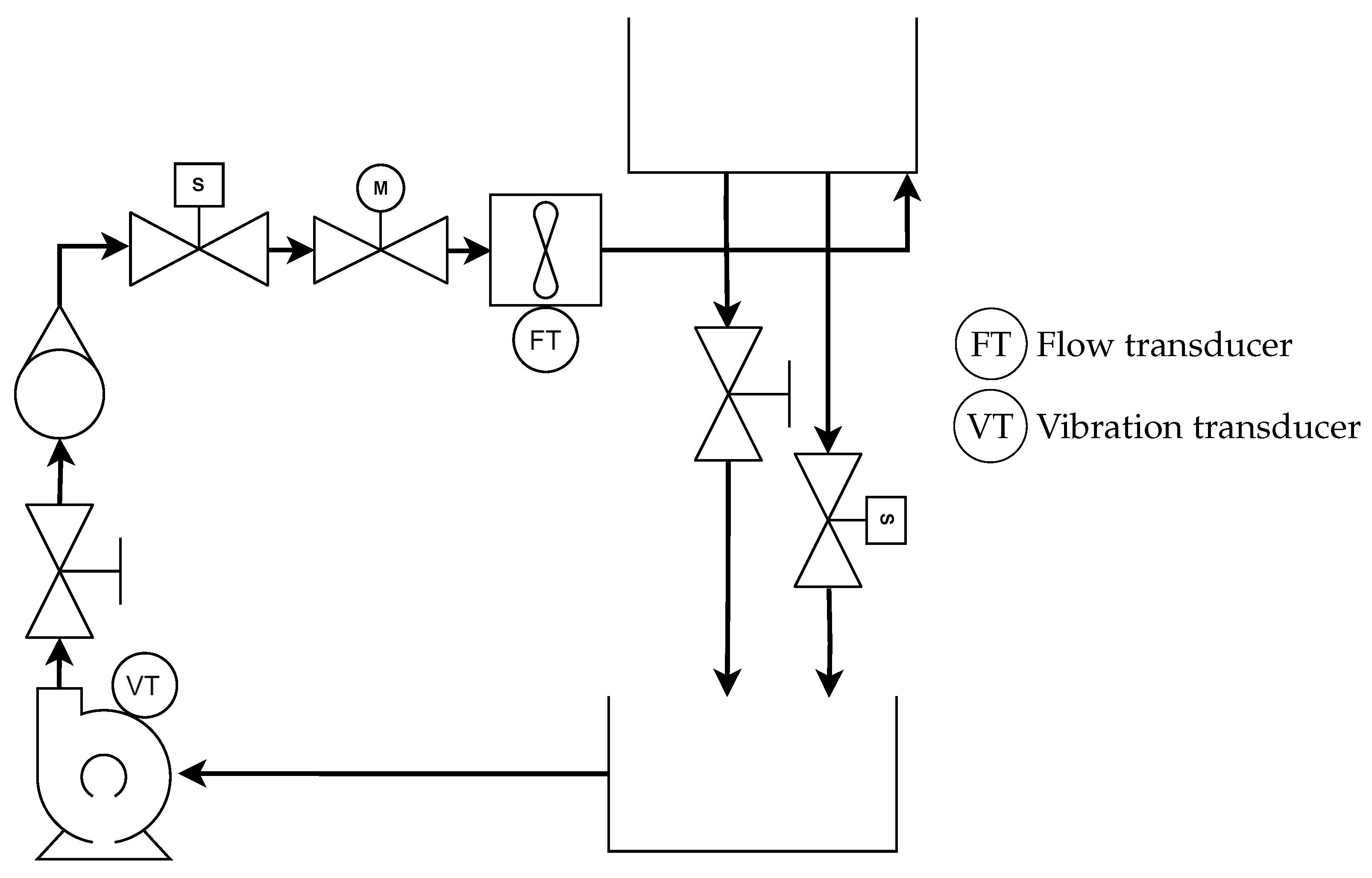
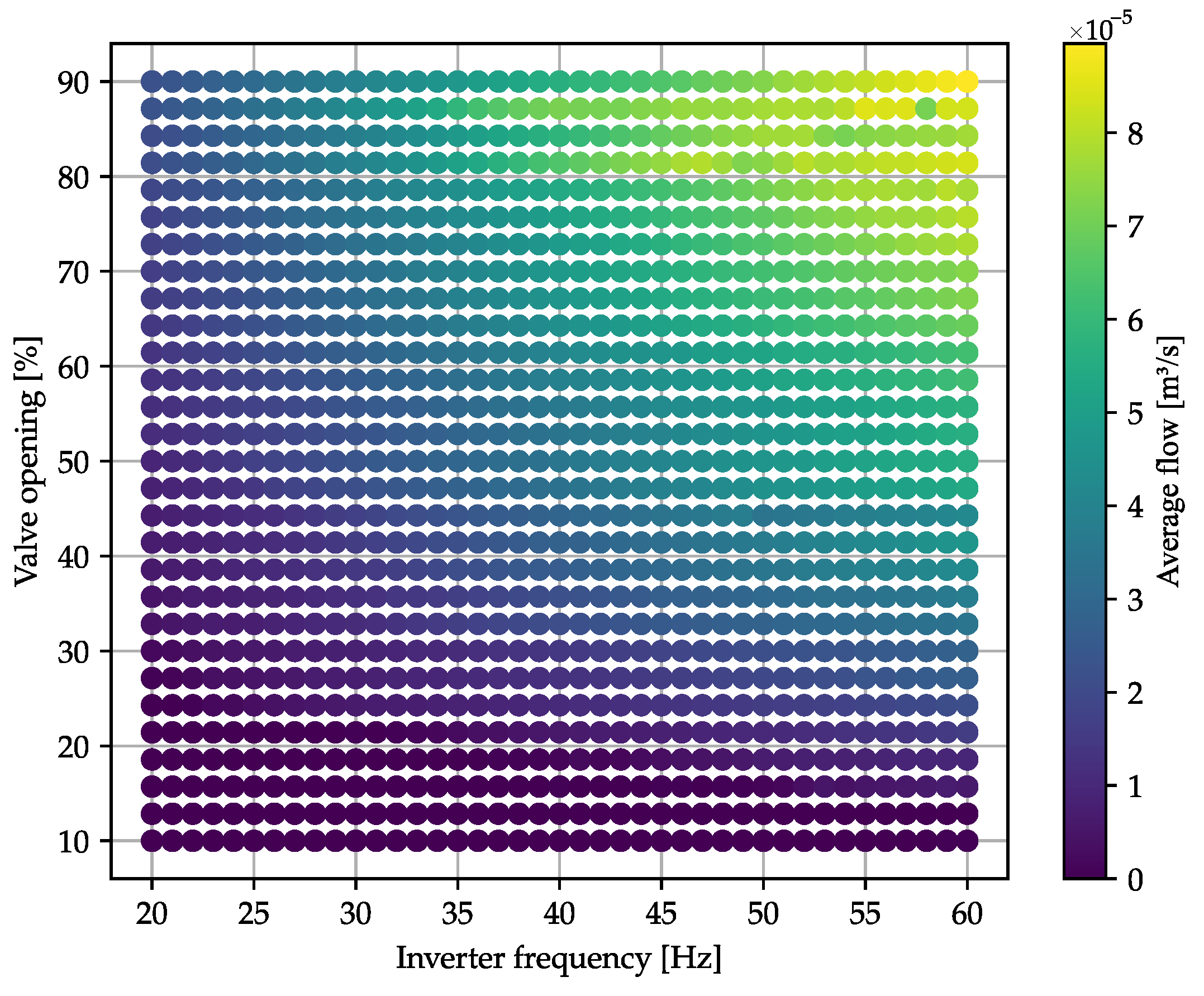
2.1. Experimental Setup

For experiments and data acquisition, a modified Armfield PCT 15 rig was used, equipped with flow and water-level control loops. This setup is designed to emulate closed-loop flow applications and operates with flow-rate values below 10 × 10⁻⁵ ${\mathrm{m}}^3$/$\mathrm{s}$, a range compatible with the areas of water service [18], smart agriculture [22], air conditioning [23], and some applications in the pharmaceutical, oil and gas, and petrochemical industries [26]. The piping and instrumentation diagram (P&ID) of the modified rig is presented in Figure 2.

The lower reservoir of the rig is used for water storage, which is suctioned and expelled by a centrifugal pump, model CAM W-4 1/4hp from Dancor, found in agricultural, industrial, urban infrastructure and residential applications. At the pump outlet, a rotameter is located to visually monitor the flow in the pipeline. Following the rotameter, a motorized valve with position control is installed, followed by a YS-201 flow transducer (indicated as FT in Figure 2), which is used to perform the actual flow measurements that define the desired reference in the development of the flow soft sensor. The flow transducer was chosen on the basis of the desired measurement range and compatibility with the test rig piping. The water is then discharged into the upper reservoir, where it can be used in a level control loop. The water returns to the lower reservoir through the existing pipes, either via manual valves or solenoid valves.

A single-phase frequency inverter model, Invertek Optidrive E3, was used to vary the operating frequency of the electric motor in the pump, thus enabling more operating conditions to be evaluated. For pump vibration measurement, a PCB M352C65 accelerometer (indicated as VT in Figure 2) was installed, with signal acquisition performed through an NI-9234 board. The accelerometer model was chosen due to its high sensitivity and accuracy, and its compatibility with the signal acquisition board, which is specifically designed for sound and vibration measurements. The test rig control and data acquisition were performed using an NI myDAQ board, with software developed by the authors in LabVIEW™.

Thirty different openings of the motorized valve, equally spaced between the occlusions 10% and 90%, were tested as a data acquisition strategy. The tests were carried out with pump motor operating frequencies between 20 $\mathrm{Hz}$ and 60 $\mathrm{Hz}$, in intervals of 1 Hz. Five vibration and flow signal acquisitions were performed for each combination of valve opening and pump motor frequency. The vibration data for the analysis were acquired over 2 $\mathrm{s}$, with a sampling rate of $25.6$ kHz.

Figure 3 presents the average flow obtained for each evaluated condition. With low valve opening (under 20%), the inverter frequency had little impact on the system flow. For all other conditions, both input variables were found to have a significant effect on the measured flow. Along with the vibration time series, these measurements were later used for training the supervised models for flow soft sensing and for uncertainty estimation, which are described further in Section 4. From this dataset, 205 combinations from the mid-flow range were chosen for the test dataset, ranging from 1.3 × 10⁻⁵ ${\mathrm{m}}^3$/$\mathrm{s}$ to 6.5 × 10⁻⁵ ${\mathrm{m}}^3$/$\mathrm{s}$.

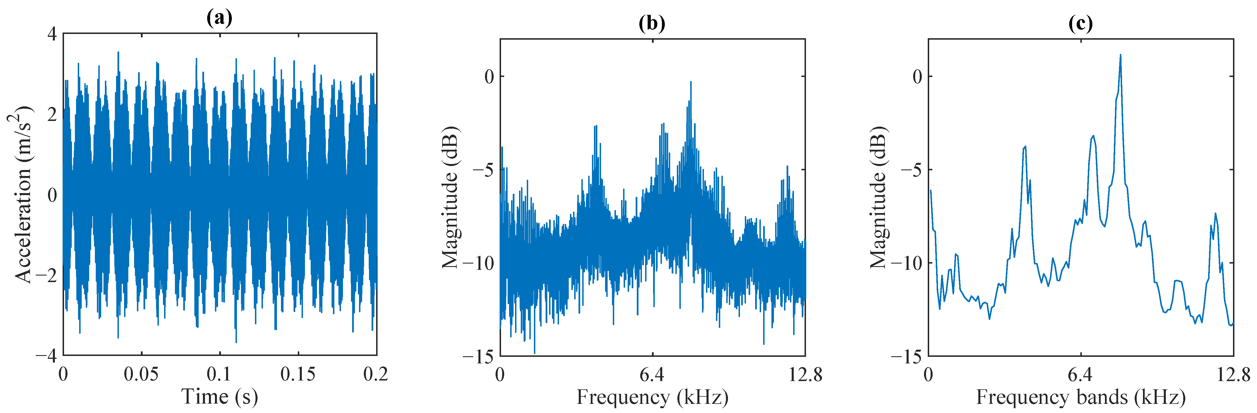
2.2. Vibration Signal Processing

The acquired data in the time domain were transformed into the frequency domain using the fast Fourier transform (FFT). This tool is suitable, under the assumption that the frequency components do not vary within the observation window, which lasts 2 $\mathrm{s}$ in this case. Taking into account the acquired vibration signal with the settings detailed in Section 2.1, the transformed signal has 25,600 points for positive frequencies. To reduce the number of inputs for the evaluated regression models, the amplitudes of adjacent frequency components were grouped into frequency bands. Different band filters were evaluated, which, in addition to condensing spectral information into fewer input parameters for the regression models, help to mitigate the impact of measurement noise for a specific filter configuration, as shown in Figure 4.

2.3. Vibration Signal Uncertainty Modeling

Let $x\left(t\right)$ represent the true acceleration signal measured by the accelerometer in the time domain. This signal is a function of the vibrations experienced by the system. In the presence of uncertainties, the observed signal $\widehat{x}\left(t\right)$ is modeled as:

$$\widehat{x}\left(t\right)=x\left(t\right)+ϵ\left(t\right),ϵ\left(t\right)\sim N(0,\sigma ),$$

(1)

where $ϵ\left(t\right)$ represents the accumulated uncertainty, with uncertainty components that affect the amplitude, phase, or other characteristics of the signal, and $N(0,\sigma )$ is a normal distribution with mean zero and standard deviation $\sigma$. The overall effect is that each component introduces a perturbation to the measured signal, which in turn affects the signal when transformed into the frequency domain via the FFT. Let $X\left(f\right)$ represent the true frequency-domain representation of the acceleration signal, obtained by applying the FFT to $x\left(t\right)$. The observed signal in the frequency domain, $\widehat{X}\left(f\right)$, is affected by the uncertainties present in the signal in the time domain $\widehat{x}\left(t\right)$. Since the Fourier transform is a linear operator, applying the FFT to $\widehat{x}\left(t\right)$, the observed signal in the frequency domain is given by [32]:

$$\widehat{X}\left(f\right)=X\left(f\right)+\mathcal{F}\left\{ϵ\left(t\right)\right\},$$

(2)

where $\mathcal{F}\left\{ϵ\right(t\left)\right\}$ represents the Fourier transform of uncertainty $ϵ\left(t\right)$, which affects the signal in the frequency domain. The total uncertainty in the frequency domain can be decomposed into two components: an amplitude perturbation and a phase perturbation.

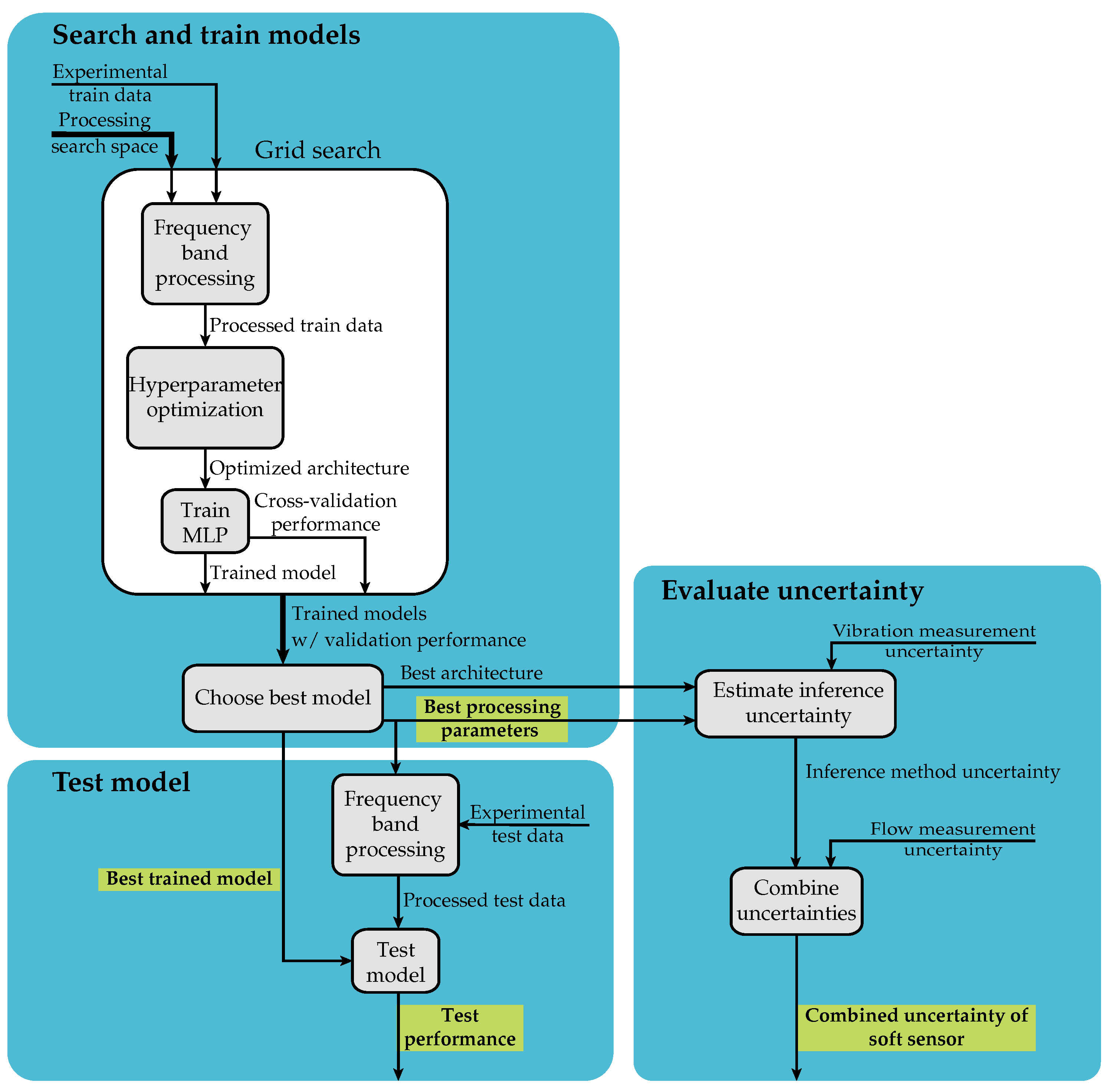
2.4. Estimation of Regression Model Uncertainty

To assess inference uncertainty, this study employs an ensemble-based method combined with MCSs. This approach, proposed in [31], uses two different ensembles of ANNs. The first ensemble generates the primary inference without incorporating input uncertainties, while the second ensemble estimates uncertainty by incorporating simulated input variability during training and during Monte Carlo evaluation. This dual setup prevents the inferred quantity from regressing toward the mean when uncertainties increase, ensuring accurate predictions under varying conditions.

The method includes MCSs and bootstrapping to account for random and systematic uncertainties in the input data. During training, MCS introduces variability by sampling from the known distribution of measurement uncertainties. Each MCS trial is paired with a bootstrap sample, creating unique training sets for each ANN in the uncertainty ensemble. This approach ensures that the propagated uncertainties accurately represent both the randomness and systematic biases in the input data, in addition to considering errors due to the incompleteness of the training set and to the process of optimization of the ANNs.

In the proposed method, the ANN ensemble is trained to model the target output, which is assumed in the training process to be a perfect representation of the actual flow rate. Thus, the standard deviation of the MCSs using the uncertainty ANN ensemble, $u_{\mathrm{E}}$, represents only the dispersion due to limitations of the training process, such as incompleteness of data coverage, optimization processes, and uncertainties in the input variables. As the target variable is, in fact, measured using a transducer which has its own accuracy with a given uncertainty distribution, it is not reasonable to assume just $u_{\mathrm{E}}$ as the standard uncertainty of the proposed soft sensor. As happens in a calibration process, which considers the accuracy of the standard transducer as a component in the uncertainty assessment of the calibrated instrument, the accuracy of the instrument used to measure the target variable, $u_{\mathrm{M}}$, is considered a component in the uncertainty assessment of the soft sensor. Since both components are statistically independent, the combined standard uncertainty of the soft sensor, $u_{\mathrm{c}\mathrm{I}}$, can be calculated as [33]:

$$u_{\mathrm{c}\mathrm{I}}=\sqrt{u_{\mathrm{M}}^2+u_{\mathrm{E}}^2}.$$

(3)

In order to reduce the training time required for implementing the soft sensor, the method presented in this paper substitutes the inference ensemble with an MLP. Despite that, the ensemble trained with bootstrapped uncertainty data and the MCSs are still employed, so matters of data inaccuracy and incompleteness as well as the optimization process during MLP training are also taken into account for the uncertainty estimation for the inference method.

3. Uncertainty Contributions

This section presents an assessment of the uncertainty in the vibration and flow measurements that were used as input for training and evaluating the flow soft sensor proposed in this work. Section 3.1 presents the uncertainty components related to vibration, while Section 3.2 presents the components related to flow measurement.

3.1. Vibration Measurement Uncertainty

In this section, the various sources of uncertainty that affect the vibration measurements of the accelerometer used in this study are presented. These uncertainties propagate through both the time-domain signal and its frequency-domain representation, influencing the accuracy of the derived flow estimates. For the accelerometer-based vibration measurement method, the uncertainty components have been extracted from the datasheet [34], and are presented in

Table 2. Accelerometer uncertainty components from [34].

Symbol	Component	Uncertainty
${\sigma }_{x,1}$	Sensitivity deviation	±10%
${\sigma }_{x,2}$	Nonlinearity	≤1%
${\sigma }_{x,3}$	Transverse sensitivity	≤5%
${\sigma }_{x,4}$	Temperature sensitivity deviation	$1\%$
${\sigma }_{x,5}$	Broadband resolution	0.0015 $\mathrm{m}$/s2
${\sigma }_{x,6}$	Base strain sensitivity	<0.05 ($\mathrm{m}$/s2)/με
${\sigma }_{x,7}$	Frequency response	$\pm 5\%$ between 0.5 and 10,000 Hz $\pm 10\%$ between 0.3 and 12,000 Hz $\pm 3$ dB between 0.2 and 20,000 Hz
${\sigma }_{x,8}$	Phase response	$\pm 5^{\circ }$
${\sigma }_{x,9}$	Spectral noise	588 (μ$\mathrm{m}$/s2)/$\sqrt{\mathrm{Hz}}$ at 1 Hz 157 (μ$\mathrm{m}$/s2)/$\sqrt{\mathrm{Hz}}$ at 10 Hz 49 (μ$\mathrm{m}$/s2)/$\sqrt{\mathrm{Hz}}$ at 100 Hz 14.7 (μ$\mathrm{m}$/s2)/$\sqrt{\mathrm{Hz}}$ at 1000 Hz

.

Despite presenting all the uncertainty components in Table 2, some considerations were taken:

• The measurements for training and using the proposed soft sensor were taken using the same accelerometer. Thus, every vibration acquisition is subject to the same sensitivity, so ${\sigma }_{x,1}$ and ${\sigma }_{x,7}$ are negligible in this context;
• The accelerometer was not moved in between measurements. Also, the dataset was constructed using the same setup. For this reason, ${\sigma }_{x,3}$ is considered to be negligible;
• The accelerometer was coupled using a magnetic base, so no considerable strain was expected for the measurement. Also, the measurements were subjected to the same strain, thus ${\sigma }_{x,6}$ was considered negligible;
• Since the power-band processing method does not require phase information, ${\sigma }_{x,8}$ was also not considered.

Excluding the above-mentioned contributions, the remaining components were considered for the uncertainty calculation. Thus, the mathematical interpretation is presented as follows.

The accelerometer is specified to have a nonlinearity of less than 1%. According to the manufacturer, the nonlinearity is taken using the zero-based, least-squares straight line method. The uncertainty due to nonlinearity, ${\sigma }_{x,2}\left(t\right)$, is given in function of the sensor’s full scale range $F_a$, and can be modeled as:

$${\sigma }_{x,2}=0.01F_a,$$

(4)

affecting the measured acceleration, particularly for large-amplitude signals.

The temperature coefficient of sensitivity means that the sensitivity of the sensor varies with temperature fluctuations. The uncertainty due to temperature deviation, ${\sigma }_{x,4}\left(t\right)$, can be modeled as:

$${\sigma }_{x,4}\left(t\right)=\alpha \mathsf{\Delta }Tx\left(t\right),$$

(5)

where $\alpha$ is the temperature coefficient and $\mathsf{\Delta }T$ is the expected temperature deviation.

The root mean squared (RMS) value of the broadband resolution of the accelerometer is specified as 0.0015 mV/(m/s²) for the frequency range of 1 Hz to 10 kHz. This represents the noise floor of the sensor, below which signals may not be distinguishable from noise. The uncertainty due to the broadband resolution, ${\sigma }_{x,5}$, can be modeled as a rectangular distribution, and so:

$${\sigma }_{x,5}={\displaystyle \frac{0.0015}{2\sqrt{3}}},$$

(6)

which adds a random perturbation to the time-domain signal, which is reflected in the frequency domain as well.

The spectral noise data provide a measure of the sensor noise at different frequencies, as presented in Table 2. The uncertainty of spectral noise, ${\sigma }_{x,9}\left(f\right)$, can be modeled as a power law function of frequency f based on these values:

$${\sigma }_{x,9}\left(f\right)=p{f}^k,$$

(7)

where p and k are adjustable parameters, with the values presented in

Table 3. Uncertainty components for different frequency ranges.

Range [Hz]	p	k
1 to 10	588.00	$-0.5735$
10 to 100	503.04	$-0.5057$
>100	544.44	$-0.5229$

.

This model captures the noise behavior over the entire frequency range. The spectral noise contribution adds uncertainty to the measured acceleration signal, particularly at lower frequencies, where noise levels are higher. The total noise contribution in a specific frequency band $[f_1,f_2]$ can be calculated as:

$${\sigma }_{x,9,\mathrm{total}}(f_1,f_2)={\left({\int }_{f_1}^{f_2}{\sigma }_{x,9}{\left(f\right)}^2\mathrm{d}f\right)}^{1/2}.$$

(8)

Aside from the aforementioned accelerometer uncertainty components, there are also uncertainty components due to signal acquisition hardware. These were taken from the datasheet provided by the manufacturer [35], considering that the equipment was calibrated, that the measurements were taken with the range of $\pm 5.1 \mathrm{V}$, and that the readings were performed in the typical temperature range (20 °C to 30 °C), and are presented in

Table 4. Acquisition uncertainty components from [35].

Symbol	Component	Uncertainty
${\sigma }_{h,1}$	Reading accuracy	$0.05\%$
${\sigma }_{h,2}$	Temperature gain drift	16 $\mathrm{p}\mathrm{p}\mathrm{m}{/}^{\circ }\mathrm{C}$
${\sigma }_{h,3}$	Analog converter resolution	24 bits
${\sigma }_{h,4}$	Master timebase accuracy	$\pm 50$ ppm maximum

. Since accelerometer data acquisition is performed using alternating coupling mode, there is no offset component, and therefore, offset uncertainties were not considered.

Given that the mean sensitivity of the accelerometer is $10.2$ $\mathrm{m}$$\mathrm{V}$/($\mathrm{m}$/s²) [34], the analog acquisition in volts, $v\left(t\right)$, and the measured acceleration in meter per second squared, $x\left(t\right)$, are proportional according to the following relation:

$$v\left(t\right)=10.2\times {10}^{-3}x\left(t\right).$$

(9)

As such, the accuracy of the acquisition can be defined in terms of acceleration as:

$${\sigma }_{h,1}\left(t\right)=0.0005v\left(t\right)=5.1\times {10}^{-6}x\left(t\right),$$

(10)

and the uncertainty due to the temperature gain drift, ${\sigma }_{h,2}\left(t\right)$, can be modeled as:

$${\sigma }_{h,2}\left(t\right)=50\times {10}^{-6}\mathsf{\Delta }Tv\left(t\right)=5.1\times {10}^{-7}\mathsf{\Delta }Tx\left(t\right).$$

(11)

Also, since the range of the acquisition hardware is $\pm 5.1 \mathrm{V}$, the analog-to-digital converter resolution, ${\sigma }_{h,3}\left(t\right)$, can be expressed in terms of acceleration as:

$${\sigma }_{h,3}\left(t\right)={\displaystyle \frac{2·5.1}{2^{24}-1}}10.2\times {10}^{-3}\approx 6.2\times {10}^{-9}\mathrm{m}/{\mathrm{s}}^2.$$

(12)

Finally, since the typical frequency of the internal master timebase of the device is $13.1072$ $\mathrm{M}$$\mathrm{Hz}$, the accuracy of the sampling period is approximately $\pm 3.8$ ps. Since the accelerometer readings were taken with a sampling frequency of $25.6$ $\mathrm{k}$$\mathrm{Hz}$ (a sampling period of approximately $0.4$ $\mathsf{\mu }$$\mathrm{s}$), the sampling deviation of the device and, consequently, the uncertainty due to the accuracy of the master timebase, ${\sigma }_{h,4}\left(t\right)$, can be considered negligible.

When comparing the aforementioned uncertainties related to the acquisition hardware and the uncertainties related to the accelerometer, it is possible to conclude that the former are at least four orders of magnitude smaller than the latter. In this case, when considering the input uncertainty components, the uncertainty of the readings due to the acquisition hardware can be considered negligible.

3.2. Flow Measurement Uncertainty

This section presents an assessment of the uncertainties related to the measurement of the liquid flow used in this study. The uncertainty components considered are presented in

Table 5. Uncertainty components from flow measurement.

Symbol	Component
${\sigma }_{f,1}$	Frequency estimation method uncertainty
${\sigma }_{f,2}$	Sensor accuracy

.

The commercial flow transducer used in the experimental setup described in Section 2.1 provides a pulse output with frequency proportional to the measured flow, with a nominal sensitivity of $7.5$ $\mathrm{Hz}$/($\mathrm{L}$/$\min$) [36]. When dealing with sensors with this characteristic, there are mainly two methods for obtaining the value of the sensor input: the frequency method, which estimates the measurand based on the number of output pulses in a given time window; and the period method, which estimates the measurand based on the period between subsequent output pulses [37].

The uncertainty component associated with the resolution of the frequency estimation method, which was used in this study, varies according to the duration of the measuring window and the number of pulses read during the time window. This component can be defined as [37]:

$${\sigma }_{f,1}={\displaystyle \frac{1}{t_{\mathrm{w}}{N}_{\mathrm{p}}}},$$

(13)

where $N_{\mathrm{p}}$ is the number of pulses per unit of measurement (9 × 10⁵ pulses/(${\mathrm{m}}^3$/$\mathrm{s}$) for the YS-F201 sensor), and $t_{\mathrm{w}}$ is the duration of the window, which was set as 2 $\mathrm{s}$ in this setup.

Finally, in the datasheet provided by the manufacturer, the accuracy of the flow sensor is given as $\pm 3\%$ [36]. Considering a rectangular distribution with mean $f\left(t\right)$ for the flow measurement, the uncertainty component associated with the sensor accuracy can then be defined based on the full scale range $F_f$ of the sensor as:

$${\sigma }_{f,2}={\displaystyle \frac{0.03F_f}{\sqrt{3}}}.$$

(14)

4. Results

Following the method described in Section 2, the experimental data obtained in the setup described in Section 2.1 were used to evaluate the proposed flow soft-sensing method based on vibration power bands. The results of the processing parameter tuning process are described in Section 4.1, along with a comparison of the proposed method against other vibration processing methods for flow soft sensing from the literature. Section 4.2 then presents an estimate for the combined uncertainty for the proposed soft-sensing method, including the individual uncertainty contributions described in Section 3 as well as the estimated uncertainty for the regression model.

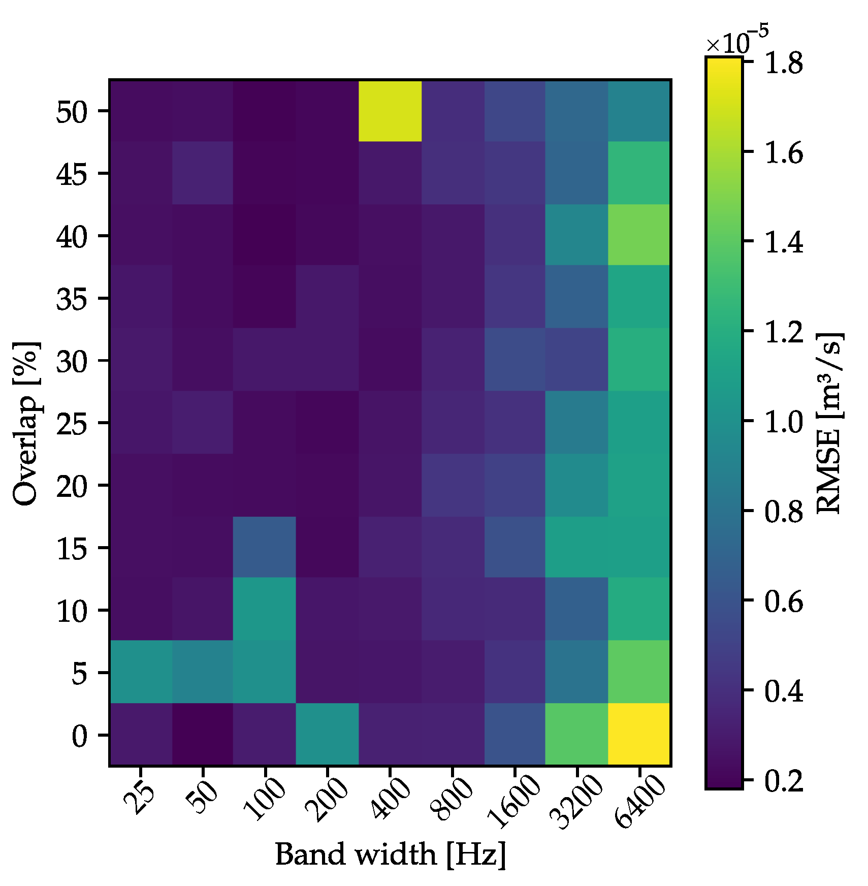
4.1. Grid Search and Hyperparameter Optimization

The search space for the grid search of the power-band parameters is presented in

Table 6. Search space for the power-band processing parameters.

Parameter	Search Space
Band width [$\mathrm{Hz}$]	{25,50,100,200,…,6400}
Band overlap [%]	{0,5,10,15,…,50}

. In order to find an optimal architecture for the MLPs, a Bayesian optimization process was run for each combination of power-band overlap and band width. The optimization space is presented in

Table 7. Optimization space for the hyperparameters of the MLP.

Hyperparameter	Optimization Space
Number of hidden layers	{1,2,3,4,5}
Neurons per hidden layer	{1,2,3,…,500}
Activation function for hidden layers	{linear, sigmoid, tanh, ReLu}
Regularization factor	(0,${10}^5$]

. Once the optimization process was completed, each model was cross-validated using k folds with $k=5$. The cross-validation error was then considered as a performance metric to find the best combination of parameters among those in the search space.

Figure 5 presents the root mean squared error (RMSE) of the cross-validation of the best models for each combination of processing parameters. The best result (RMSE of 0.182 × 10⁻⁵ ${\mathrm{m}}^3$/$\mathrm{s}$) was obtained with a power-band width of 50 $\mathrm{Hz}$ and no overlap. Then, this combination of parameters was chosen to process the data in the flow soft sensor.

The performance of the soft sensor with power-band processing was compared with models trained using different processing methods described in the literature, i.e., the RMS value of vibration [38], the frequency and amplitude of the first harmonic [39,40], and the low-frequency components of the vibration FFT [41]. In addition to these processing methods, a model was also trained using the full FFT spectrum of the vibration. The same MLP hyperparameter optimization process used for the power-band model was used to evaluate the other processing methods. The results of all methods are presented in

Table 8. Performance comparison between prediction models with different vibration processing methods.

Processing Method	Cross-Validation RMSE [m³/s]	Test RMSE [m³/s]
RMS [38]	2.066 × 10−5	1.443 × 10−5
Fundamental amplitude [39]	2.184 × 10−5	1.278 × 10−5
Fundamental amplitude and frequency [40]	1.890 × 10−5	0.994 × 10−5
RMS and fundamental amplitude and frequency	1.974 × 10−5	1.128 × 10−5
FFT (Full spectrum)	0.738 × 10−5	0.802 × 10−5
FFT (under 100 Hz) [41]	1.636 × 10−5	1.419 × 10−5
Power band	0.182 × 10−5	0.389 × 10−5

, with the best results highlighted. For easier visual comparison, the same results are graphically presented in Figure 6.

The two processing methods with the smaller errors were the power-band and the full FFT spectrum methods, both in cross-validation and in test, but the power band resulted in a significantly smaller error than the full FFT (75.4% smaller in cross-validation and 51.5% in the test dataset). Compared with the processing methods with the largest error, which were the fundamental amplitude for cross-validation and the RMS for testing, the power band resulted in an error 91.7% and 73.0% smaller for cross-validation and testing, respectively. It should also be noted that the training and optimization time of the MLP when the input was the full FFT spectrum was significantly larger than all other methods due to the larger number of input nodes in the input layer, and might be impractical for datasets with large frequency resolution (high sampling frequency and long sampling window).

Once the estimation capability of the model with the power-band processing method was validated, the uncertainty of the model was estimated using the ensemble and Monte Carlo method proposed in [31]. This evaluation of the uncertainty is presented in Section 4.2.

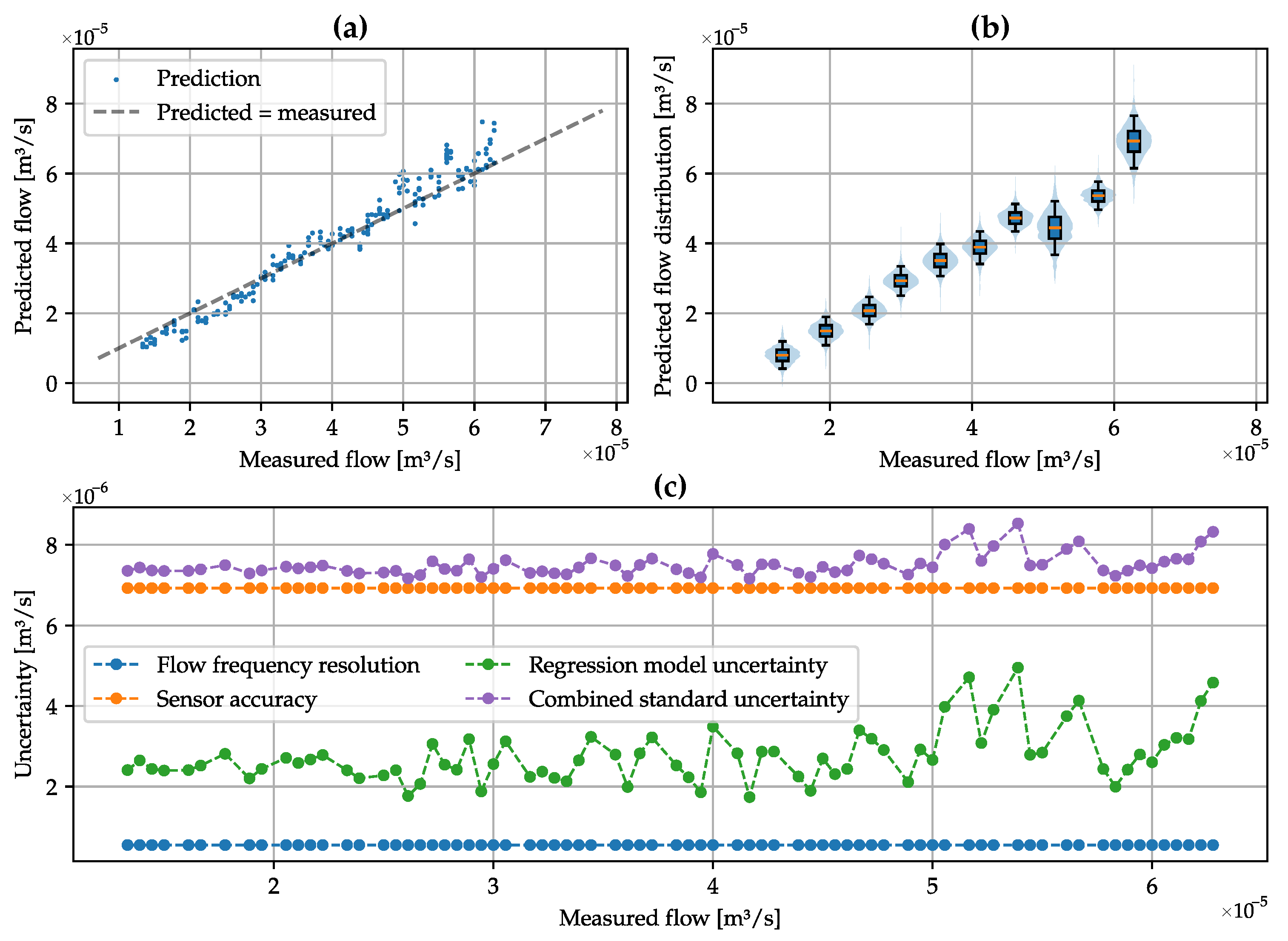
4.2. Uncertainty Evaluation

The uncertainty of the inference was estimated using an ensemble of ${10}^3$ models and ${10}^3$ MCSs per model, resulting in ${10}^6$ MCSs per prediction. The uncertainty components of the vibration described in Section 3.1 were considered in both ensemble training and MCSs, as discussed in Section 2.4.

Figure 7a presents the predictions from the proposed soft sensor. It can be seen that the ideal prediction line falls close to the ideal prediction line, especially when close to the middle of the evaluated flow range. Figure 7b presents violin and box plots for a sample of 10 predicted values, with the space between the upper and lower whiskers representing the 95% confidence interval. These plots show that the distribution of the predicted flow for each case resembles a Gaussian distribution, with a larger standard deviation when estimating larger flow values.

Figure 7c presents the individual uncertainty contributions of the soft-sensor model, as well as the combined uncertainty. The uncertainty due to the accuracy of the flow sensor was the largest contributor to the combined uncertainty of the system, at 6.93 × 10⁻⁶ ${\mathrm{m}}^3$/$\mathrm{s}$. The uncertainty of the regression model, taken as the standard deviation of the MCSs in the uncertainty inference ensemble, was found to be between 1.74 × 10⁻⁶ ${\mathrm{m}}^3$/$\mathrm{s}$ and 4.95 × 10⁻⁶ ${\mathrm{m}}^3$/$\mathrm{s}$, and was significantly larger for some larger flow conditions. In general, the combined uncertainty for the soft-sensor model was found to be slightly smaller for low flow values than for larger ones, staying between 7.16 × 10⁻⁶ ${\mathrm{m}}^3$/$\mathrm{s}$ and 8.53 × 10⁻⁶ ${\mathrm{m}}^3$/$\mathrm{s}$ throughout the measured flow range.

5. Conclusions

This paper presents a study on the use of virtual sensing techniques with machine learning tools to estimate fluid flow rate based on vibration data acquired on the surface of a centrifugal pump. The dataset was acquired using a test rig adapted for the problem. For acquisition under different operating conditions, the opening of the flow control valve and the pump operating frequency were varied. With the system in the testing condition, simultaneous measurements of vibration and flow rate were made.

To extract frequency-domain features for the regression models, the acquired vibration time series were processed using band filters with different widths and overlaps. The amplitude values of the frequency bands were used as input for different regression models and evaluated in a grid search for each regression technique. The proposed method was evaluated using MLPs with hyperparameters optimized through Bayesian optimization for each preprocessing condition in the grid search, using the RMSE obtained in cross-validation as the optimization metric.

The RNA models were used for regression on a test set composed of experimental measurements at a valve opening different from those used in training and validation. The model with the lowest RMSE in cross-validation was compared with other frequency-based processing methods from the literature and was found to reduce the RMSE by 75.4% in cross-validation and 51.5% in tests compared to the second-best processing method evaluated.

Using an ensemble trained with uncertainty data and bootstrapping, MCSs were performed on the test dataset to evaluate the uncertainty of the regression model. The uncertainty due to the reference sensor accuracy was found to be the largest contributor to the combined uncertainty of the soft sensor in general. The regression model uncertainty was found to be between 1.74 × 10⁻⁶ ${\mathrm{m}}^3$/$\mathrm{s}$ and 4.95 × 10⁻⁶ ${\mathrm{m}}^3$/$\mathrm{s}$, and was more significant for larger flow values. In general, the combined uncertainty of the model was found to be between 7.16 × 10⁻⁶ ${\mathrm{m}}^3$/$\mathrm{s}$ and 8.53 × 10⁻⁶ ${\mathrm{m}}^3$/$\mathrm{s}$. While the flow rate range in this study is relatively low compared to some applications listed in Table 1, the methodology demonstrates adaptability and could be extended to higher flow rate systems or other domains, such as industrial processes or environmental monitoring, by accounting for system-specific variations and requirements.

Future work will consider processing data in octave bands, typically used to assess the vibration spectrum of rotating machinery to obtain information about its rotational speed, and the addition of the other non-invasive measurements to the model, such as the electric power of the centrifugal pump and the pressure in the system. Another line of future research involves the exploration of unsupervised or semi-supervised learning models. For instance, clustering methods or autoencoders could be employed to identify patterns in the vibration and flow data, while semi-supervised frameworks could incorporate limited labeled data for fine-tuning. These approaches could mitigate the dependency on large labeled datasets, since data labeling is often time-consuming or costly, enabling broader applicability of the developed methods in industrial and research contexts.

References

1. Chowdhury, W.S.; Yan, Y.; Coster-Chevalier, M.A.; Liu, J. Mass flowrate measurement of slurry using coriolis flowmeters and data driven modeling. IEEE Trans. Instrum. Meas. 2024, 73, 1–12. [Google Scholar] [CrossRef]
2. Baker, R.C. Positive Displacement Flowmeters. In Flow Measurement Handbook: Industrial Designs, Operating Principles, Performance, and Applications; Cambridge University Press: Cambridge, UK, 2000; pp. 182–214. [Google Scholar]
3. Chen, B.; Zhou, Y.; Huang, T.; Ying, S.; Chen, T. Technical features and application of electromagnetic flow meter. In Proceedings of the 2020 International Conference on Communications, Information System and Computer Engineering (CISCE), Kuala Lumpur, Malaysia, 3–5 July 2020; pp. 1–5. [Google Scholar] [CrossRef]
4. Gu, X.; Cegla, F. The uncertainties induced by internal pipe wall roughness on the measurements of clamp-on ultrasonic flow meters. In Proceedings of the 2019 IEEE International Ultrasonics Symposium (IUS), Glasgow, UK, 16–19 October 2019; pp. 1586–1589. [Google Scholar] [CrossRef]
5. Li, Z.; Jin, H.; Dong, S.; Qian, B.; Yang, B.; Chen, X. Semi-supervised ensemble support vector regression based soft sensor for key quality variable estimation of nonlinear industrial processes with limited labeled data. Chem. Eng. Res. Des. 2022, 179, 510–526. [Google Scholar] [CrossRef]
6. Mozharovskii, I.; Shevlyagina, S. A hybrid approach to soft sensor development for distillation-in-series plant under input data low variability. Meas. Sci. Technol. 2024, 35, 076211. [Google Scholar] [CrossRef]
7. Sangiorgi, L.; Sberveglieri, V.; Carnevale, C.; De Nardi, S.; Nunez-Carmona, E.; Raccagni, S. Data-driven virtual sensing for electrochemical sensors. Sensors 2024, 24, 1396. [Google Scholar] [CrossRef]
8. Vijayan, S.V.; Mohanta, H.K.; Rout, B.K.; Pani, A.K. Adaptive soft sensor design using a regression neural network and bias update strategy for non-linear industrial processes. Meas. Sci. Technol. 2023, 34, 085012. [Google Scholar] [CrossRef]
9. Karatzas, S.; Merino, J.; Puchkova, A.; Mountzouris, C.; Protopsaltis, G.; Gialelis, J.; Parlikad, A.K. A virtual sensing approach to enhancing personalized strategies for indoor environmental quality and residential energy management. Build. Environ. 2024, 261, 111684. [Google Scholar] [CrossRef]
10. Berrie, P. 3-Sensors for automated food process control: An introduction. In Robotics and Automation in the Food Industry; Caldwell, D.G., Ed.; Woodhead Publishing Series in Food Science, Technology and Nutrition; Woodhead Publishing: Cambridge, UK, 2013; pp. 36–74. [Google Scholar] [CrossRef]
11. Wang, D.; Kang, Q.; Yang, J.; Gong, J.; Zhang, Q. Research on data-driven model for soft sensing of natural gas production system. Eng. Rep. 2022, 4, e12495. [Google Scholar] [CrossRef]
12. Flores, T.K.S.; Villanueva, J.M.M.; Gomes, H.P.; Catunda, S.Y.C. Indirect feedback measurement of flow in a water pumping network employing artificial intelligence. Sensors 2021, 21, 75. [Google Scholar] [CrossRef]
13. Chen, T.C.; Alizadeh, S.M.; Alanazi, A.K.; Grimaldo Guerrero, J.W.; Abo-Dief, H.M.; Eftekhari-Zadeh, E.; Fouladinia, F. Using ANN and combined capacitive sensors to predict the void fraction for a two-phase homogeneous fluid independent of the liquid phase type. Processes 2023, 11, 940. [Google Scholar] [CrossRef]
14. Ling, T.; Qian, C.; Schiele, G. Towards auto-building of embedded FPGA-based soft sensors for wastewater flow estimation. In Proceedings of the 2024 IEEE Annual Congress on Artificial Intelligence of Things (AIoT), Melbourne, Australia, 24–26 July 2024; pp. 248–249. [Google Scholar] [CrossRef]
15. Alencar, G.M.R.d.; Fernandes, F.M.L.; Moura Duarte, R.; Melo, P.F.d.; Cardoso, A.A.; Gomes, H.P.; Villanueva, J.M.M. A soft sensor for flow estimation and uncertainty analysis based on artificial intelligence: A case study of water supply systems. Automation 2024, 5, 106–127. [Google Scholar] [CrossRef]
16. Lima, J.S.; Villanueva, J.M.M.; Catunda, S.Y.C. Modeling a virtual flow sensor in a sugar-energy plant using artificial neural network. In Proceedings of the 2022 IEEE International Instrumentation and Measurement Technology Conference (I2MTC), Ottawa, ON, Canada, 16–19 May 2022; pp. 1–6. [Google Scholar] [CrossRef]
17. Zheng, D.; Shao, S.; Liu, A.; Wang, M.; Li, T. Soft measurement model for wet gas flow rate based on ultrasonic and differential pressure sensing. Meas. Sci. Technol. 2024, 35, 055003. [Google Scholar] [CrossRef]
18. Lima, R.P.G.; Mauricio Villanueva, J.M.; Gomes, H.P.; Flores, T.K.S. Development of a soft sensor for flow estimation in water supply systems using artificial neural networks. Sensors 2022, 22, 3084. [Google Scholar] [CrossRef]
19. Manami, M.; Seddighi, S.; Örlü, R. Deep learning models for improved accuracy of a multiphase flowmeter. Measurement 2023, 206, 112254. [Google Scholar] [CrossRef]
20. Andrade, G.M.; de Menezes, D.Q.; Soares, R.M.; Lemos, T.S.; Teixeira, A.F.; Ribeiro, L.D.; Vieira, B.F.; Pinto, J.C. Virtual flow metering of production flow rates of individual wells in oil and gas platforms through data reconciliation. J. Pet. Sci. Eng. 2022, 208, 109772. [Google Scholar] [CrossRef]
21. Gilbert Chandra, D.; Vinoth, B.; Srinivasulu Reddy, U.; Uma, G.; Umapathy, M. Recurrent neural network based soft sensor for flow estimation in liquid rocket engine injector calibration. Flow Meas. Instrum. 2022, 83, 102105. [Google Scholar] [CrossRef]
22. Chen, X.; Wei, Z.; Wei, C.; He, K. Machine learning approaches to estimate flow rate of drip irrigation emitter based on structure parameters and pressure. J. Phys. Conf. Ser. 2022, 2203, 012017. [Google Scholar] [CrossRef]
23. Liu, Z.; Tan, H.; Li, Z.; Jiang, K. Water pump flow monitoring method for air conditioning system based on parameter model. Sustain. Cities Soc. 2020, 61, 102166. [Google Scholar] [CrossRef]
24. Ren, W.; Su, W.; Sun, H.; Liu, C.; Lu, X.; Hua, Y. Soft sensing model of flow rate for independent metering valves based on LSTM. In Proceedings of the 2023 9th International Conference on Fluid Power and Mechatronics (FPM), Lanzhou, China, 18–21 August 2023; pp. 1–4. [Google Scholar] [CrossRef]
25. Deng, C.; Chen, G.; Liu, S.; Yao, Z.; Zhang, W.; lu, Z.; Wu, S. Operating flow rate prediction of H4 condition in NPP. J. Phys. Conf. Ser. 2023, 2520, 012044. [Google Scholar] [CrossRef]
26. Jiang, Y.; Wang, H.; Liu, Y.; Peng, L.; Zhang, Y.; Chen, B.; Li, Y. A flow rate estimation method for gas–liquid two-phase flow based on transformer neural network. IEEE Sens. J. 2024, 24, 26902–26913. [Google Scholar] [CrossRef]
27. Gandhi, M.; Mathew, A.; Chaudhari, S.; Shaik, R.; Vattem, A. IoT and ML-based water flow estimation using pressure sensor. In Proceedings of the 2023 IEEE 20th India Council International Conference (INDICON), Hyderabad, India, 14–17 December 2023; pp. 892–897. [Google Scholar] [CrossRef]
28. Lu, D.; Su, L. A novel flow rate measurement method for fire hose based on vibration signal and neural network. Flow Meas. Instrum. 2024, 97, 102600. [Google Scholar] [CrossRef]
29. Gawlikowski, J.; Tassi, C.R.N.; Ali, M.; Lee, J.; Humt, M.; Feng, J.; Kruspe, A.; Triebel, R.; Jung, P.; Roscher, R.; et al. A survey of uncertainty in deep neural networks. Artif. Intell. Rev. 2023, 56, 1513–1589. [Google Scholar] [CrossRef]
30. Sagi, O.; Rokach, L. Ensemble learning: A survey. Wires Data Min. Knowl. Discov. 2018, 8, e1249. [Google Scholar] [CrossRef]
31. Pacheco, A.L.S.; Flesch, R.C.C.; Flesch, C.A.; Iervolino, L.A.; Barros, V.T. Tool based on artificial neural networks to obtain cooling capacity of hermetic compressors through tests performed in production lines. Expert Syst. Appl. 2022, 194, 116494–116510. [Google Scholar] [CrossRef]
32. Lathi, B.P. Linear Systems and Signals, 2nd ed.; Oxford University Press, Inc.: New York, NY, USA, 2009. [Google Scholar]
33. ISO. Evaluation of Measurement Data—Guide to the Expression of Uncertainty in Measurement; Vol. JJCGM 100:2008; International Organization for Standardization: Geneva, Switzerland, 2008. [Google Scholar]
34. PCB Piezotronics Inc. Product Data: ICP Accelerometer Model 352C65. 2024. Available online: https://www.pcb.com/contentStore/docs/pcb_corporate/vibration/products/specsheets/m352c65_l.pdf (accessed on 10 November 2024).
35. National Instruments Corp. NI-9234 Specifications. 2023. Available online: https://www.ni.com/docs/en-US/bundle/ni-9234-specs/page/specs.html (accessed on 10 November 2024).
36. Sea Electronics Inc. YF-S201 Flow Sensor Specifications. 2020. Available online: https://abg.baidu.com/view/a7390ef3ba0d4a7302763adf (accessed on 10 November 2024).
37. Machado, J.P.Z.; Thaler, G.; Pacheco, A.L.S.; Flesch, R.C.C. Impact of angular speed calculation methods from encoder measurements on the test uncertainty of electric motor efficiency. Metrology 2024, 4, 164–180. [Google Scholar] [CrossRef]
38. Dinardo, G.; Fabbiano, L.; Vacca, G.; Lay-Ekuakille, A. Vibrational signal processing for characterization of fluid flows in pipes. Measurement 2018, 113, 196–204. [Google Scholar] [CrossRef]
39. Campagna, M.M.; Dinardo, G.; Fabbiano, L.; Vacca, G. Fluid flow measurements by means of vibration monitoring. Meas. Sci. Technol. 2015, 26, 115306. [Google Scholar] [CrossRef]
40. Evans, R.P.; Blotter, J.D.; Stephens, A.G. Flow rate measurements using flow-induced pipe vibration. J. Fluids Eng. Trans. ASME 2004, 126, 280–285. [Google Scholar] [CrossRef]
41. Venkata, S.K.; Navada, B.R. Estimation of flow rate through analysis of pipe vibration. Acta Mech. Autom. 2018, 12, 294–300. [Google Scholar] [CrossRef]
Figure 1. A diagram of the proposed method.
Metrology 05 00006 g001
Figure 2. The P&ID of the experimental test rig. The flow transducer (FT) measures the real-time flow rate for further model training, while the vibration transducer (VT) captures pump vibration data to serve as input.
Metrology 05 00006 g002
Figure 3. The average flow for the evaluated experimental conditions.
Metrology 05 00006 g003
Figure 4. Vibration data processing: (a) vibration signal in the time domain; (b) amplitude spectrum of the vibration signal FFT; (c) frequency bands from the FFT, calculated with a width of 100 Hz and a 5% overlap.
Metrology 05 00006 g004
Figure 5. Cross-validation errors for different power-band processing parameters.
Metrology 05 00006 g005
Figure 6. Comparison of vibration processing methods for flow estimation using MLP.
Metrology 05 00006 g006
Figure 7. The uncertainty estimation for the trained model: (a) soft-sensor predictions; (b) the predicted distribution of 10 samples; (c) the individual and combined uncertainties of the proposed soft-sensing method.
Metrology 05 00006 g007