Plantar Load System Analysis Using FSR Sensors and Interpolation Methods

Abstract

The foot is considered a wonder of biological engineering due to its structure, formed by bones, ligaments, and tendons that collaborate to ensure stability and mobility. A key area often examined by medical professionals in patients with diabetic feet is the plantar surface, due to the risk of ulcer development. If left untreated, these ulcers can lead to severe complications, including amputation of the toe, foot, or even the limb. Interpolation methods are used to find areas with overloads in a system of sensor maps that are based on capacitive, load cells, or force-sensitive resistors (FSRs). This manuscript presents the assessment of linear, nearest neighbors, and bicubic methods in comparison with ground truth to calculate the root mean square error (RMSE) in two assessments using a dataset of eight healthy subjects, four men and four women, with an average age of 25 years, height of 1.63 m, and weight of 72 kg with shoe sizes from 7.3 USA using FSR map with 48 sensors. Additionally, this paper describes the conditioning circuit development to implement a plantar surface system that enables interpolating loads on the plantar surface. The proposed system’s results show that the first assessment indicates an RMSE of 0.089, 0.126, and 0.089 for linear, nearest neighbor, and bicubic methods, while the second assessment shows a mean RMSE for linear, nearest neighbor, and bicubic methods of 0.114, 0.159, and 0.112.

1. Introduction

Feet play a crucial role in mobility and balance; they are the foundation for daily activities such as running and walking. The feet are essential for maintaining equilibrium. Consequently, any impairment in foot health can have a profound impact on life quality. Therefore, in medical fields, reliable systems are required to provide precise measurement and monitoring of plantar pressure to identify areas at risk. These areas of risk caused by overload on the plantar surface can cause ulcers in diabetic feet [1,2,3]. If this condition remains untreated, it may result in limb amputation. To address this issue, orthopedics or podiatry use instruments such as a podoscope or flexible sensors configured in either a matrix or individual setup. The podoscope allows for qualitative plantar load determination through visual analysis, while matrix or individual sensors enable quantitative measurement of the load on the plantar surface [4,5,6,7]. These sensors can be load cells, capacitive sensors, or flexible sensitive resistive (FSR) sensors. The work [8] describes a detection system for capacitive plantar pressure monitoring that presents better results in terms of linear behavior under applied pressure. The publication [9] introduces a novel unit that utilizes eight load cells to measure the load distribution on the rearfoot, midfoot, and forefoot, enabling the classification of different foot types. The research [10] introduces a 32 × 32 map of FSR sensors, which form a matrix to measure the distribution of foot pressure during both dynamic and static activities. This technology enables a detailed analysis of pressure patterns, which is helpful in developing targeted interventions to mitigate the risk of ulcerations. To analyze the regions with overload on the plantar surface, interpolation methods are applied, including linear, bilinear, bicubic, and nearest neighbor [11,12,13,14]. A research paper on the analysis of interpolation methods for a flexible sensor map shows that these several approaches can be used to obtain improved outcomes in image quality. The research employs these algorithms to transform sensor data into a higher-resolution pressure matrix. Therefore, it improves understanding of pressure distribution on the plantar surface [15]. Although interpolation methods are widely used in plantar analysis, these present differences that must be considered. For example, the bilinear and nearest neighbor methods are less used, while bicubic interpolation is the most preferred in many applications, as it produces higher quality images because it employs polynomial interpolation [16,17,18,19]. However, the processing of the bicubic method requires more computational resources, which makes real-time measurements difficult [20,21,22,23]. On the other hand, the comparison between interpolation methods and ground truth has not been determined. Therefore, the assessment of linear, nearest neighbor, and bicubic methods in comparison with ground truth was used to calculate the root mean square error (RMSE) in two assessments using a dataset of eight healthy subjects, four men and four women, with an average age of 25 years, a height of 1.63 m, and a weight of 72 kg, with shoe sizes from 7.3 USA, using an FSR map with 48 sensors. The second contribution of this manuscript is the development of the conditioning circuits and software of the system based on the FSR sensor map to determine the load plantar by applying linear, nearest neighbor, and bicubic interpolation methods.

2. Materials and Methods

The plantar pressure system is composed of two conditioning circuits and two FSR sensor insoles distributed on the plantar surface, along with one foam cover and a plastic cover that protects the FSR sensors, as shown in Figure 1a,b. The system uses the RS232 protocol to transmit the measurements from each sensor to a LabVIEW program, which then interpolates the data.

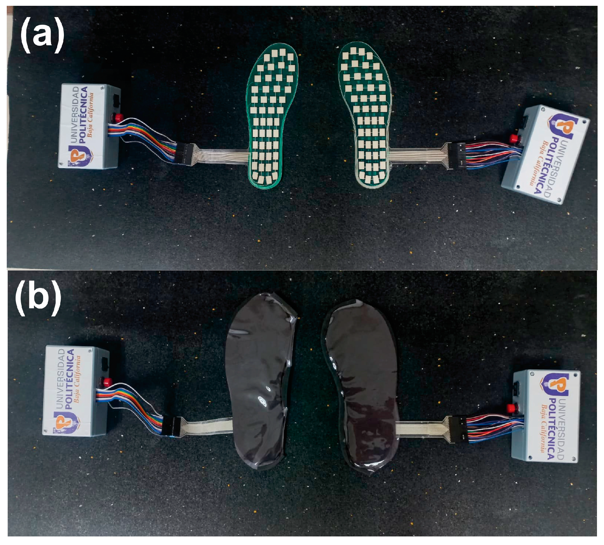
2.1. Plantar Load Insole

Similar to other studies [24,25,26,27,28], this system uses a plantar load insole with 48 FSR sensors placed on the plantar surface. Each sensor provides a resistance value in response to the exerted load, which varies from 1 MΩ to 0 Ω in a range of 0 to 10 kg.

Table 1. Technical characteristics of the FSR sensors.

Performance Parameter	Parameter Value
Static Resistance	1 MΩ
Hysteresis	Less than 6%
Drift	Less than 8%
Sensor Repeatability	±8%
Working Voltage	3.3 V–5 V
Working Temperature	−50 °C–60 °C
Working Humidity	0–95%
Response Time	Less than 20 ms
Lifespan	More than 500,000 cycles

presents additional technical characteristics of the sensor FSRs.

For interpolation methods, it is necessary to select an origin in the insole for assigning a coordinate to each sensor, as shown in Figure 2. Here, the sensors are enumerated to localize their corresponding coordinates on the insole.

2.2. Conditioning Circuit

The developed conditioning circuit is composed of one microcontroller, four voltage dividers, and one LM324 Quad OP-AMP. The sensors are connected to 40 kΩ resistors of ¼ watt to form voltage dividers. To create a voltage divider in each column of the plantar pressure insole, it is necessary to energize the rows with 3.3 volts at different instances, considering the response time of the sensor. This procedure is performed using the 12 digital outputs of a microcontroller, which individually energizes the rows, each for 25 ms, enabling the complete sampling of all sensors in 300 ms. The outputs of the voltage dividers are connected to an LM324 integrated circuit in a buffer configuration to maintain the current when the voltage is low. Finally, the output of the LM324 is connected to the analog input of the microcontroller with a 12-bit ADC. In general, while the digital output energizes the rows, the analog input reads the signal and the ADC converts it to a digital signal with a resolution of 0 to 4095 value, which is then converted to load units. A schematic of the connected devices in the conditioning circuit is shown in Figure 3.

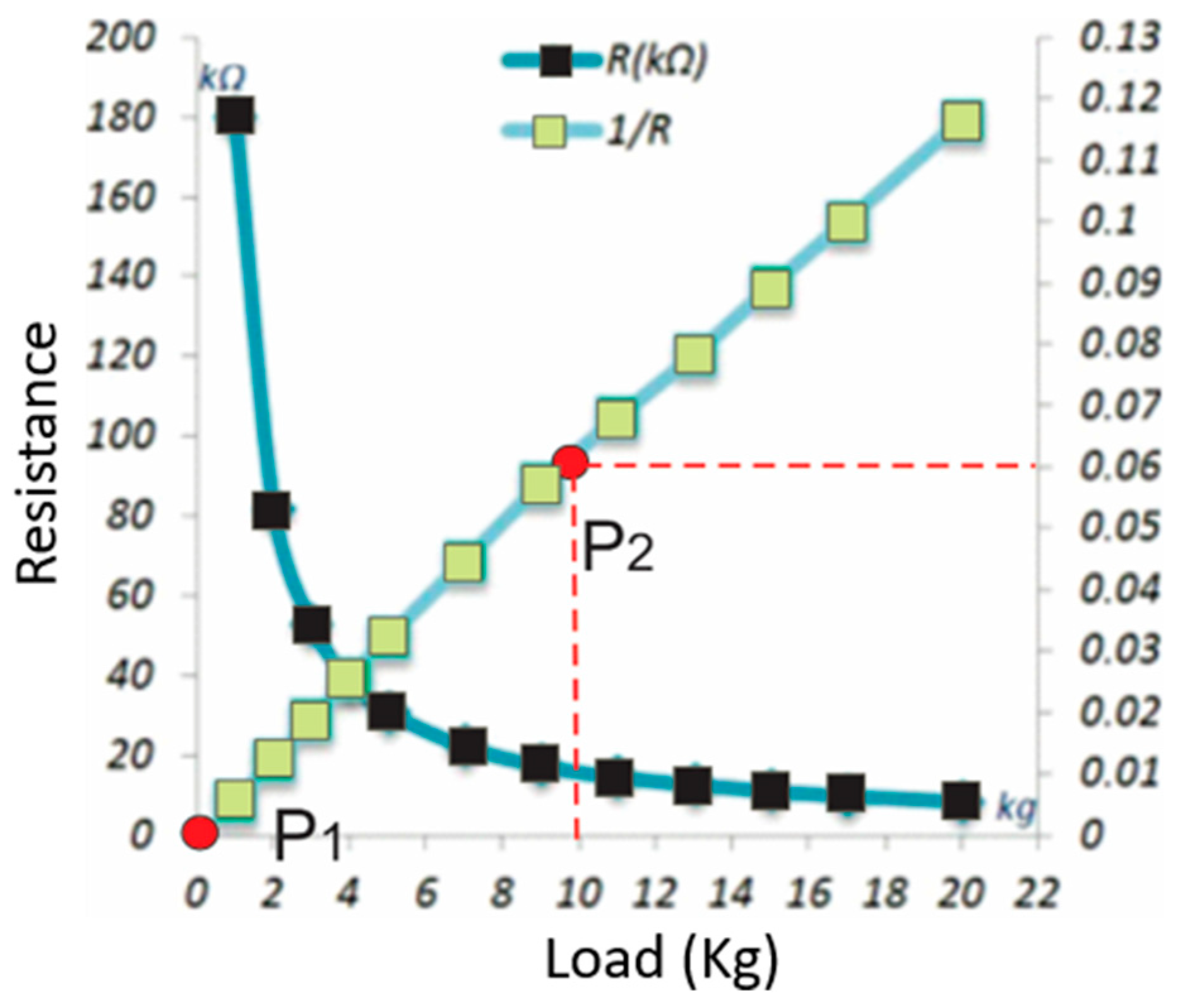
2.3. Conversion of Resistance to Load Units

The developed interface in LabVIEW receives four sensor measurements at different times until forming a matrix dimension of 12 × 4, which corresponds to a sampling of all sensors. These values are converted to a voltage unit by applying Equation (1). Where R is a scalar that represents the DAC resolution, which in our case is 12 bits (4095). Vcc is also a scalar that represents the maximum supply of the DAC. $R{m}_{12\times 4}$ is a matrix with dimensions 12 × 4 that indicates the measured resolution value, and $Vou{t}_{12\times 4}$ is a matrix of 12 × 4 that represents the output voltage.

$$Vou{t}_{12\times 4}={\displaystyle \frac{\left(Vcc\right)\left(R{m}_{12\times 4}\right)}{R}}$$

(1)

The $Vou{t}_{12\times 4}$ matrix is utilized to compute a resistance matrix for the FSR sensors by employing the voltage divider equation to determine $R_2$, as denoted in Equation (2). In this context, Vin and R1 are scalar values representing the input voltage of 5 volts and the resistance of ¼ watt in the voltage divider equation. The matrix $R{2}_{12\times 4}$ represents the resistance values of the FSR sensors in relation to the applied load.

$$R{2}_{12\times 4}={\displaystyle \frac{\left(Vou{t}_{12\times 4}\right)\left(R1\right)}{Vin-Vou{t}_{12\times 4}}}$$

(2)

In accordance with the flexible sensors’ datasheet, the load varies linearly with conductance. Therefore, the reciprocal of the voltage matrix is calculated by applying Equation (3). This procedure enables the creation of a conductance matrix $C_{12\times 4}$.

$$C_{12\times 4}={\displaystyle \frac{1}{R{2}_{12\times 4}}}$$

(3)

Additionally, a linear regression method is applied using the characteristic curvature provided by the supplier (Figure 4) to develop a mathematical model that calculates the load depending on the conductance and kilograms, as shown in Equation (4), where $Y_{12\times 4}$ represents the load value in kilograms.

$$Y_{12\times 4}={\displaystyle \frac{C_{12\times 4}}{0.006}}$$

(4)

The matrix $Y_{12\times 4}$ and the sensor coordinates are employed with interpolation methods such as bilinear, nearest neighbor, and bicubic. These methods are applied to a 60 × 60 mesh to plot the loads in each cell using a color palette.

2.4. Interpolation Methods

The interpolation methods applied to estimate load are linear, bilinear, nearest neighbor, and bicubic. However, these methods vary as load estimation depends on different mathematical models. For example, linear interpolation consists of two known points and assumes that the value change of form is linear to calculate the unknown value by using Equation (5). Where ($x_{0 }$, $y_0$) represents the coordinates of the first point, ($x_1, y_1$) represents the coordinates of the second point, x is the point at which to perform the interpolation, and y is the interpolated value [29,30].

$$y=y_0+{\displaystyle \frac{\left(y_1-y_0\right)}{\left(x_1-x_0\right)}}\left(x-x_0\right)$$

(5)

The nearest neighbor is a direct and simple interpolation method that assigns the value of the closest data point. It is suitable for applications where simplicity and speed are prioritized over result smoothness [31,32]. To determine the closest point at the point $p$, it is necessary to calculate the Euclidean distances of all points; the point closest ($p_{nearest}$) is the interpolated value $f\left(p\right)$ as shown in Equation (6).

$$f\left(p\right)=f\left(p_{nearest}\right)$$

(6)

The bicubic method is a mathematical model used for interpolating points in a 2D grid. The results are smoother compared to those obtained using nearest-neighbor methods. However, it requires more computational resources [33,34,35]. The bicubic method is expressed by Equation (7), where $a_{ij}$ is the coefficient of the polynomial, x and y are the coordinates of the point to interpolate, and i and j are indices used to denote positions in a grid of data points surrounding the point where interpolation is being performed.

$$f\left(x,y\right)={\sum }_{i=0}^3{\sum }_{j=0}^3{a}_{ij}{x}^i{y}^j$$

(7)

Using a first-order equation, linear interpolation smooths transitions between two points, hence improving accuracy. However, the bicubic interpolation approach utilizes a larger number of data points and a third-order polynomial equation, resulting in an even higher accuracy for this application. Conversely, the foot size helps explain the low RMSE since more sensors are in contact with the surface plantar, facilitating interpolations with a low RMSE for every evaluation.

2.5. Software

The software receives information from the sensors via the serial port, creating a 12 × 4 matrix. This matrix is then processed by the equations outlined in Section 2.4, allowing for the visualization of interpolation and the evaluation of interpolated values to determine the system’s performance. The interfaces feature a color map that displays sensor values and interpolated values to identify overload. This interface enables the storage of the measurements in a matrix of 12 × 4 for each 300 ms.

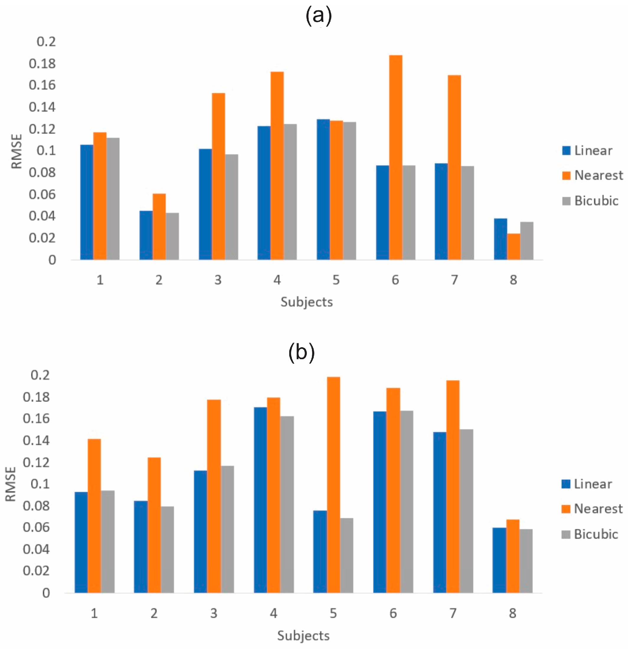
2.6. Ground Truth vs. Interpolation Methods

The assessment of interpolation methods in relation to the ground truth includes the evaluation of 10 specific spots on the insole. The data points are derived from sensors that were excluded, leaving only 38 sensors for interpolation. The central coordinates of the excluded sensors and their measurements are subsequently utilized to compare the interpolated values at these coordinates. The first evaluation uses ten center coordinates of the excluded sensors as the internal ground truth, as highlighted in blue in Figure 5a. The second evaluation uses ten center coordinates of the excluded sensors as external ground truth and their measurements, also highlighted in blue, as shown in Figure 5b. The evaluations exclude the external points highlighted in red (Figure 5c), as these points present NAN values with the interpolation methods applied.

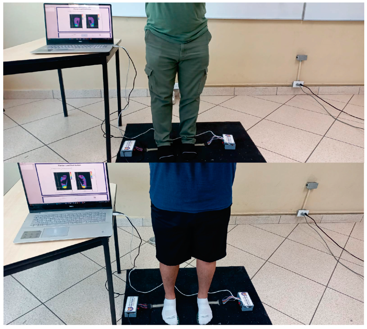
3. Experimentation and Results

The experiment was carried out on a 1 × 0.6 m rubber mat, where the load insole of 48 flexible FSR sensors was placed along with the developed conditioning circuits and software. The experiment was performed on eight healthy subjects, four men and four women, with an average age of 25 years, a height of 1.63 m, a weight of 72 kg, and shoe sizes from 7.3 USA (

Table 2. Physical characteristics of the subjects.

Subject	Weight (kg)	Height (m)	Shoe Size (Inches)
1	60	1.62	7
2	96	1.74	9.5
3	88	1.65	6.5
4	64	1.49	6.5
5	50	1.58	6
6	55	1.52	4
7	90	1.76	9
8	73	1.72	9.5

). During the experimentation, the subjects were measured while maintaining body equilibrium, as shown in Figure 6. As the first contribution, these measurements were used to compare the ground truth with the obtained measurements from the linear, nearest neighbor, and bicubic interpolation methods. The dataset created in this study is available in the Supplementary Materials (Dataset S1).

The first assessment was conducted using thirty-eight sensors for interpolation and ten internal FSR sensors (ground truth). The comparison is conducted by calculating the root mean square error (RMSE) between the ten sensors and the interpolation values in the same coordinates.

Table 3. RMSE values of the interpolation methods with respect to internal FSR sensors.

Subject	Linear (kg)	Nearest Neighbor (kg)	Bicubic (kg)
1	0.086	0.122	0.086
2	0.045	0.061	0.043
3	0.102	0.153	0.097
4	0.123	0.173	0.125
5	0.129	0.128	0.127
6	0.087	0.188	0.087
7	0.089	0.170	0.086
8	0.038	0.024	0.035

shows the RMSE values in kilograms of the interpolation methods with respect to the ten internal sensors across the eight subjects.

The second assessment was also conducted using thirty-eight sensors for interpolation and ten external FSR sensors (ground truth). The comparison is performed by calculating the RMSE between the 10 sensors and interpolation values in the same coordinate with eight subjects.

Table 4. RMSE values of the interpolation methods with respect to external FSR sensor.

Subject	Linear (kg)	Nearest Neighbor (kg)	Bicubic (kg)
1	0.093	0.142	0.094
2	0.085	0.125	0.080
3	0.113	0.178	0.117
4	0.171	0.180	0.163
5	0.076	0.199	0.069
6	0.167	0.189	0.168
7	0.148	0.196	0.151
8	0.060	0.068	0.059

shows the RMSE values in kilograms of the interpolation methods with respect to the ten external sensors across the eight subjects.

The RMSE values of the eight subjects in the first assessment by applying the three interpolation methods are shown in Figure 7a. Also, the RMSE values of the eight subjects in the second assessment with the three interpolation methods are shown in Figure 7b.

For the first assessment using internal FSR sensors, the average RMSE for the eight people was 0.089 for the linear method, 0.126 for the nearest neighbor method, and 0.089 for the bicubic method. The second assessment’s result with external FSR sensors shows a mean RMSE for linear, nearest neighbor, and bicubic methods of 0.114, 0.159, and 0.112, respectively. The linear and bicubic methods present similar RMSE values in their respective assessments, while the nearest neighbor method indicates a greater RMSE than the other methods for each assessment. Moreover, the correlations between foot sizes and RMSE values indicate −0.654, −0.705, and −0.657 for linear, nearest neighbor, and bicubic methods. These coefficients represent a negative correlation between the two variables, indicating a moderate inverse relationship between foot sizes and the obtained RMSE values. This means that as foot size increases, errors tend to decrease, or vice versa.

The second manuscript contribution introduces the FRS sensors and interpolated values on a color map, allowing for a visual comparison of the interpolated method and regions with overloads on the plantar surface across eight subjects. Figure 8a–c shows an example of a color map of subject one by applying the linear, nearest neighbor, and bicubic methods of the first assessment with 38 sensors, excluding ten internal sensors. Furthermore,

Table 5. Comparison between internal ground truth and interpolation methods for subject one.

Ground Truth (kg)	x Position	y Position	Linear Interpolation (kg)	Nearest Interpolation (kg)	Bicubic Interpolation (kg)
0.196	−2.5	−1.3	0.096	0.185	0.100
0.280	−0.4	−3.5	0.212	0.245	0.171
0.191	−1.9	−5.2	0.112	0.190	0.113
0.204	0.2	−0.7	0.111	0.000	0.156
0	−0.9	−8.7	0.099	0.185	0.076
0.185	0.2	−10.6	0.134	0.000	0.144
0	−1.1	−12.5	0.095	0.000	0.102
0.268	0.3	−14.5	0.245	0.302	0.262
0.545	−0.8	−16.3	0.436	0.435	0.452
0.567	0.3	−18.2	0.457	0.729	0.428

displays the sensors’ ten measurements (ground truths) and ten interpolation values in the same location as the ground truths. The same procedure was performed in subject one with 38 sensors, excluding ten external sensors. The color map obtained by applying linear, nearest neighbor, and bicubic methods for the second assessment is shown in Figure 9a–c, respectively. Moreover,

Table 6. Comparison between external ground truth and interpolation methods for subject one.

Ground Truth (kg)	x Position	y Position	Linear Interpolation (kg)	Nearest Interpolation (kg)	Bicubic Interpolation (kg)
0.233	1.4	−3.5	0.152	0.285	0.152
0	−3.8	−5.2	0.029	0.000	0.043
0	−2.4	−8.7	0.065	0.000	0.056
0.278	1.5	−10.6	0.216	0.185	0.211
0	−2.2	−10.6	0.107	0.000	0.093
0.235	1.3	−12.5	0.204	0.223	0.202
0	−2.2	−12.5	0.157	0.000	0.160
0.215	1.5	−16.3	0.118	0.435	0.116
0.438	−2	−16.3	0.509	0.545	0.523
0.205	1.5	−17.8	0.064	0.567	0.063

shows a comparison between ground truths and interpolation values, similar to Table 5.

4. Discussion

The root mean square error (RMSE) values for the two assessments indicated that the nearest neighbor method has a greater error compared to the linear and bicubic methods. Moreover, Figure 7a,b shows that the nearest neighbor method exhibits a higher error for almost every measured subject in the two assessments. On the other hand, the correlation between the interpolated values and foot sizes is −0.654, −0.705, and −0.657 for the linear, nearest neighbor, and bicubic methods, respectively. The results between the two variables indicate that the correlation between foot size and RMSE value shows that RMSE lowers as foot size rises. This occurs since this experiment made use of a 9.5″ insole. Consequently, feet smaller than 9.5″ have less contact with the plantar surface, and feet sized 9.5″ have more contact with the whole surface. Fewer sensors available for interpolation from this reduced contact cause a larger RMSE. On the other hand, for future interpolation methods in medical evaluations, using an insole size that fits the subject’s foot size will help to ensure that all sensors make contact with the entire plantar surface for accurate measurements.

Another finding in this research is that the sensors shown in Figure 5c are excluded because they cannot be used as the ground truth. This occurs due to the presence of NAN values in some interpolation sites when using external coordinates. The reason for these NAN values is the inability of interpolation methods to reliably predict values in the absence of internal data. The absence of data interpolation in contour zones of the plantar surface hinders the effectiveness of medical evaluation in predicting foot ulcers in individuals with diabetes resulting from excessive load. Therefore, it is recommended to avoid making estimations in contour shapes and instead make use of physical sensors. Finally, the load measurement in each assessment can be illustrated on a color map, as shown in Figure 8 and Figure 9. These examples are performed with the measurements of subject one, which indicates that the three interpolation methods using the first and second assessments present visual differences. The linear method presents a load on the contour of the plantar arch greater than the color map of the bicubic method, while the color map of the nearest neighbor method does not make it possible to visualize this load. Moreover, the color map generated by the nearest neighbor method exhibits roughness because this method only considers the nearest point, unlike linear and bicubic methods, which take into account values from surrounding points. Finally, it is important to consider the sensors’ parameters because they can impact the comparison of the obtained results. Furthermore, only one measurement cycle was performed per subject in the experiment; therefore, results may vary with additional measurement cycles.

5. Conclusions

This manuscript presents a plantar load system evaluated using interpolation methods with different configurations of the ground truth. The results obtained from four men and four women, with an average age of 25 years, an average height of 1.63 m, and an average weight of 72 kg with shoe sizes of 7.3 US, indicate that the bicubic and linear methods present a lower root mean square error (RMSE) compared to the nearest neighbor method in the two assessments performed. Moreover, the correlation indicates that the RMSE tends to decrease as foot size increases or vice versa. Additionally, this study suggests that to get accurate measurements, the insole size should be matched to the subject’s plantar surface size, and the sensor measurements of the contours should be used instead of interpolation predictions. This is because interpolation methods cannot predict values in external data.

References

1. Reddie, M.; Frey, D. A resource-efficient plantar pressure evaluation system for diabetic foot risk assessment. Diabetology 2024, 5, 206–222. [Google Scholar] [CrossRef]
2. Lockhart, M.; Dinneen, S.F.; O’Keeffe, D.T. Plantar pressure measurement in diabetic foot disease: A scoping review. J. Diabetes Investig. 2024, 8, 990–999. [Google Scholar] [CrossRef]
3. Tang, J.; Bader, D.L.; Moser, D.; Parker, D.J.; Forghany, S.; Nester, C.J.; Jiang, L. A wearable insole system to measure plantar pressure and shear for people with diabetes. Sensors 2023, 23, 3126. [Google Scholar] [CrossRef]
4. Musaid, R.; Ghazwan, A.; Al-Saadan, W.A. A low-cost podoscope for extracting morphological features of the foot. Period. Eng. Nat. Sci. 2023, 11, 269–280. [Google Scholar] [CrossRef]
5. Musaid, R.; Ghazwan, A.; Al-Saadan, W.A. Assessment of foot deformities in patients with knee osteoarthritis. Al-Khwarizmi Eng. J. 2024, 20, 73–85. [Google Scholar] [CrossRef]
6. Smondrk, M.; Babusiak, B.; Kreanova, A.; Janousek, L. Design of instrumented insole for gait dynamics monitoring. Lékař Technika 2024, 54, 17–21. [Google Scholar] [CrossRef]
7. Luo, H.; Zhang, X.; Xu, Y.; Yu, J.; Ma, X.; Chen, W.M. A novel flexible multidimensional force platform for assessing regional plantar pressure and shear stress under the foot during gait. IEEE Sens. J. 2024, 24, 11723–11733. [Google Scholar] [CrossRef]
8. Feng, Z.; He, Q.; Wang, X.; Lin, Y.; Qiu, J.; Wu, Y.; Yang, J. Capacitive sensors with hybrid dielectric structures and high sensitivity over a wide pressure range for monitoring biosignals. ACS Appl. Mater. Interfaces 2023, 15, 6217–6227. [Google Scholar] [CrossRef]
9. Trujillo-Hernández, G.; Rodríguez-Quiñonez, J.C.; Flores-Fuentes, W.; Sergiyenko, O.; Ontiveros-Reyes, E.; Real-Moreno, O.; Rascón, R. Development of an integrated podometry system for mechanical load measurement and visual inspection. Measurement 2022, 203, 111866. [Google Scholar] [CrossRef]
10. Ortiz-Villaseñor, D.; Rodríguez-Quiñonez, J.C.; Trujillo-Hernández, G.; Hernandez-Balbuena, D.; Flores-Fuentes, W.; Sanchez-Castro, J.J. Measurement of plantar pressures through FSR sensors and spatial resolution through interpolation. In Proceedings of the 2024 IEEE 33rd International Symposium on Industrial Electronics (ISIE), Ulsan, Republic of Korea, 18 June 2024. [Google Scholar]
11. Earshia, V.D.; Sumathi, M. A comprehensive study of 1D and 2D image interpolation techniques. In ICCCE 2018: Proceedings of the International Conference on Communications and Cyber Physical Engineering 2018; Springer: Singapore, 2018; Volume 500, pp. 383–391. [Google Scholar]
12. Patil, M.S.M.M. Interpolation techniques in image resampling. Int. J. Eng. Technol. 2018, 7, 567–570. [Google Scholar]
13. Hajizadeh, M.; Helfroush, M.S.; Tashk, A. Improvement of image zooming using least directional differences based on linear and cubic interpolation. In Proceedings of the 2009 2nd International Conference on Computer, Control and Communication, Karachi, Pakistan, 17 February 2009. [Google Scholar]
14. Azam, N.Z.F.N.; Yazid, H.; Rahim, S.A. Super resolution with interpolation-based method: A review. IJRAR 2022, 9, 168–174. [Google Scholar]
15. Fatema, A.; Kuriakose, I.; Gupta, R.; Hussain, A.M. Analysis of interpolation techniques for a flexible sensor mat for plantar pressure measurement. In Proceedings of the 2023 IEEE Applied Sensing Conference (APSCON), Bengaluru, India, 13 January 2023. [Google Scholar]
16. Triwijoyo, B.K.; Adil, A. Analysis of medical image resizing using bicubic interpolation algorithm. J. Ilmu Komput. 2021, 14, 20–29. [Google Scholar] [CrossRef]
17. Kang, X.; Li, S.; Hu, J. Fusing soft-decision-adaptive and bicubic methods for image interpolation. In Proceedings of the 21st International Conference on Pattern Recognition (ICPR2012), Tsukuba, Japan, 11 November 2012. [Google Scholar]
18. Hisham, M.B.; Yaakob, S.N.; Raof, R.A.; Nazren, A.B.; Wafi, N.M. An analysis of performance for commonly used interpolation method. Adv. Sci. Lett. 2017, 23, 5147–5150. [Google Scholar] [CrossRef]
19. Al-Hadaad, M.H.; Thabit, R.; Zidan, K.A. A new face region recovery algorithm based on bicubic interpolation. JOIV 2023, 7, 1000–1006. [Google Scholar] [CrossRef]
20. Weng, S.E.; Ye, Y.G.; Lin, Y.C.; Miaou, S.G. Reducing computational requirements of image dehazing using super-resolution networks. In Proceedings of the 2023 Sixth International Symposium on Computer, Consumer and Control, Taichung, Taiwan, 30 June 2023. [Google Scholar]
21. Zhu, Y.; Dai, Y.; Han, K.; Wang, J.; Hu, J. An efficient bicubic interpolation implementation for real-time image processing using hybrid computing. J. Real-Time Image Process. 2022, 19, 1211–1223. [Google Scholar] [CrossRef]
22. Guo, A.; Lin, E.; Zhang, J.; Liu, J. An energy-efficient image filtering interpolation algorithm using domain-specific dynamic reconfigurable array processor. Integration 2024, 96, 102167. [Google Scholar] [CrossRef]
23. Huang, Z.; Cao, L. Bicubic interpolation and extrapolation iteration method for high resolution digital holographic reconstruction. Opt. Lasers Eng. 2020, 130, 106090. [Google Scholar] [CrossRef]
24. Mahmud, S.; Khandakar, A.; Chowdhury, M.E.; AbdulMoniem, M.; Reaz, M.B.I.; Mahbub, Z.B.; Alhatou, M. Fiber Bragg Gratings based smart insole to measure plantar pressure and temperature. Sens. Actuators A Phys. 2023, 350, 114092. [Google Scholar] [CrossRef]
25. Hu, X.; Duan, Q.; Tang, J.; Chen, G.; Zhao, Z.; Sun, Z.; Qu, X. A low-cost instrumented shoe system for gait phase detection based on foot plantar pressure data. IEEE J. Transl. Eng. Health Med. 2023, 12, 2168–2372. [Google Scholar] [CrossRef]
26. Jang, C.W.; Park, K.; Paek, M.C.; Jee, S.; Park, J.H. Validation of the Short Physical Performance Battery via Plantar Pressure Analysis Using Commercial Smart Insoles. Sensors 2023, 23, 9757. [Google Scholar] [CrossRef]
27. Cho, H. Walking speed estimation and gait classification using plantar pressure and on-device deep learning. IEEE Sens. J. 2023, 23, 23336–23347. [Google Scholar] [CrossRef]
28. Darwich, A.; Ismaiel, E.; Al-kayal, A.; Ali, M.; Masri, M.; Nazha, H.M. Recognizing different foot deformities using FSR sensors by static classification of neural networks. Baghdad Sci. J. 2023, 20, 2638. [Google Scholar] [CrossRef]
29. Hernández, P.A.Q. Métodos Numéricos con Aplicaciones en Excel; Reverte: Barcelona, Spain, 2005; pp. 1–263. [Google Scholar]
30. Steiner, E. Matemáticas para las Ciencias Aplicadas; Reverte: Barcelona, Spain, 2018; pp. 1–624. [Google Scholar]
31. Bhabatosh, C. Digital Image Processing and Analysis; PHI Learning Pvt. Ltd.: Delhi, India, 2011; Volume 1, pp. 1–469. [Google Scholar]
32. Esfandiari, R.S. Numerical Methods for Engineers and Scientists Using MATLAB®; CRC Press: Boca Raton, FL, USA, 2017; pp. 1–493. [Google Scholar]
33. Aizawa, K.; Nakamura, Y.; Satoh, S.I. (Eds.) Advances in Multimedia Information Processing-PCM 2004: 5th Pacific Rim Conference on Multimedia, Tokyo, Japan, 30 November–3December 2004, Proceedings; Springer Science & Business Media: Tokyo, Japan, 2004; pp. 1–1323.
34. Shapiro, L. (Ed.) Computer Vision and Image Processing; Academic Press: New York, NY, USA, 1992; pp. 1–431. [Google Scholar]
35. Ota, K.; Ukai, T.; Wakai, T. Spatial resolution improvement by a super-resolution technique depending on training process in the background-orientated schlieren analyses. Phys. Fluids 2023, 35, 126103. [Google Scholar] [CrossRef]
Figure 1. (a) Insoles with 48 FSR sensors. (b) Foam and plastic cover for the insole.
Metrology 04 00035 g001
Figure 2. FSR sensor coordinates in the plantar load insole.
Metrology 04 00035 g002
Figure 3. This conditioning circuit is composed of a microcontroller, four 40 k Ω resistances, one LM324 Quad OP-AMP.
Metrology 04 00035 g003
Figure 4. Characteristic curvature kilograms versus conductance. The FSR sensors’ load capacity leads to the selection of P 1 and P 2 which define the linear equation.
Metrology 04 00035 g004
Figure 5. (a) First evaluation with internal ground truth. (b) Second evaluation with external ground truth. (c) External FSR sensor with NAN values with interpolation methods.
Metrology 04 00035 g005
Figure 6. Experimentation was performed on eight healthy subjects.
Metrology 04 00035 g006
Figure 7. (a) Obtained RMSE values for the first assessment. (b) Obtained RMSE values for the second assessment.
Metrology 04 00035 g007
Figure 8. (a) Internal ground truth: (a) linear, (b) nearest neighbor, (c) bicubic.
Metrology 04 00035 g008
Figure 9. (a) External ground truth: (a) linear, (b) nearest neighbor, (c) bicubic.
Metrology 04 00035 g009