An Artificial Neural Network-Based Approach to Improve Non-Destructive Asphalt Pavement Density Measurement with an Electrical Density Gauge

Abstract

Asphalt pavement density can be measured using either a destructive or a non-destructive method. The destructive method offers high measurement accuracy but causes damage to the pavement and is inefficient. In contrast, the non-destructive method is highly efficient without damaging the pavement, but its accuracy is not as good as that of the destructive method. Among the devices for non-destructive measurement, the nuclear density gauge (NDG) is the most accurate, but radiation in the device is a serious hazard. The electrical density gauge (EDG), while safer and more convenient to use, is affected by the factors other than density, such as temperature and moisture of the environment. To enhance its accuracy by minimizing or eliminating those non-density factors, an original approach based on artificial neural networks (ANNs) is proposed. Density readings, temperature, and moisture obtained by the EDG are the inputs, and the corresponding densities obtained by the NDG are the outputs to train the ANN models through Levenberg-Marquardt, Bayesian regularization, and Scaled Conjugate Gradient algorithms. Results indicate that the ANN models trained greatly improve the measurement accuracy of the electrical density gauge.

1. Introduction

Asphalt pavement’s density is commonly measured with the destructive coring method (CM) [1]. In this method, the core samples are taken from the asphalt pavement and sent to a laboratory for density measurement [2,3,4]. Although it has a high measurement accuracy, it is time-consuming and causes damage to the pavement, which needs to be repaired after the measurement [5].

This problem is solved with the so-called highly efficient non-destructive methods relying on the readings of specialized devices such as the nuclear density gauge (NDG) and the electrical density gauge (EDG). The NDG contains a nuclear radiation source, which emits gamma photons on the pavement. The density is measured through the count of the back-scattered gamma photons [1,6]. Though the measurement is accurate, the internal radiation poses hazards to the operators [7]. Unlike NDG, EDG measures density based on the variation of the parameters of an electric field with the density of the asphalt pavement [8]. It is safe to use, however, its readings are affected by environmental factors such as temperature, and moisture [1,9].

Unlike EDG, some non-destructive methods are based on mechanical wave propagation, including the ultrasonic pulse velocity (UPV) and the impact-echo methods [10]. The UPV device includes two transducers, which can be placed onto the same or opposite surface(s) of the measured material. When the measurement starts, the ultrasonic pulses, transformed from voltage pulses, are transmitted by the first transducer and received by the second transducer. By analyzing the transmission time of the pulses, the strength of the received pulses, and the distance between the two transducers, some properties of the measured material can be characterized. The impact-echo method is developed based on the UPV method and has the ability to measure the properties of a multilayer material [10]. The impact-echo device only includes one transducer. Ultrasonic pulses are transmitted by the transducer and are reflected after encountering the boundary of another layer. Then, the reflected pulses are received by the same transducer, and their strength and transition time are recorded. Both of the methods have been applied to measure the properties of cement concrete [10]. However, their performance in measuring the density of the asphalt pavement requires further investigation.

This research focuses on improving the currently applied non-destructive method, which is EDG. Considering its advantages, an original approach based on artificial neural network (ANN) is developed to address the issues mentioned above. ANN is a data-driven approach, which means a large amount (from hundreds to thousands) of data samples are required to train an ANN [11]. Thus, a time-consuming data-collocation process is required, which is a limitation of using ANN. Conversely, one of the advantages of using ANN is that it has a self-learning ability. Although the relationship between the input and target data (EDG and NDG densities) is complicated, ANN has the ability to automatically reduce the error between them by exploring the potential features of the data samples [11]. Furthermore, using ANN also has the advantage of working efficiency. The relationship between input and target data can be accurately described by ANN models, which are established in less than one second. Hence, an ANN approach is selected as a basement to develop the proposed approach.

In the proposed approach, the ANN models consisting of one input layer, two hidden layers, and one output layer are adopted. The input data for training the ANN models include EDG density readings, temperature, and moisture. Subsequently, the ANN models output the predicted density, which is then compared with the NDG density readings. The errors between them are used to tune the ANN model parameters through the Levenberg-Marquardt (LM), the Bayesian regularization (BR), and the Scaled Conjugate Gradient (SCG) algorithms [12,13,14], producing the LM-ANN model, the BR-ANN model, and the SCG-ANN model, respectively.

The LM algorithm aims to enhance the accuracy of the current input data by exploring as many features as possible [12,15]. However, this can lead to overfitting problems, where the model fits the training data too closely and performs poorly on new data, resulting in reduced generalization capability. In contrast, the BR-ANN model maintains a relatively balanced accuracy and generalization capability, albeit requiring a relatively longer training process [13]. Additionally, the SCG-ANN model can be trained efficiently and exhibits good generalization capability, although its accuracy is comparatively lower [14]. To accommodate the varying features of the three models, their structures are optimized by adjusting the number of neurons in each hidden layer, ranging from 3 to 30. Each model is trained 100 times, and the average performance is subsequently analyzed. Finally, models with optimized structures are selected, and their performances are evaluated and compared with the original performance of the EDG.

The paper is organized as follows. In Section 2, non-destructive devices NDG and EDG are described. In Section 3, the ANN approach is presented in terms of the ANN structure, training process, learning algorithms, and input data. Then, the methodology of the proposed approach is described in Section 4, including the methods to optimize the structure of the ANN models and evaluate the performance of the optimized models. After that, the performances of the optimizing and the optimized models are evaluated and discussed in Section 5. Finally, a conclusion is drawn in Section 6.

2. Non-Destructive Devices

2.1. Nuclear Density Gauge (NDG)

The nuclear density gauge (NDG) is a non-destructive device designed to operate on the surface of asphalt pavement, as depicted in Figure 1 [6,7]. The left part of the NDG includes the control panel, including a small 2-key keypad, a 20-key keypad, and a small screen. The 2-key keypad is used to power on or off the NDG. The 20-key keypad contains the number keys (from 0 to 9 and a decimal point) and the functional keys (Yes, No, Start, Offset, etc.). The number keys are used to enter the project number, current time, manual offset, etc. The functional keys are used to accept a measurement result or not (Yes or No), start a new measurement, set the offset manually, etc. The small screen can display the measurement results and the status of the NDG. The right part of the NDG includes the nuclear source rod with a black handle. The source rod can be lifted up or down via the handle and locked into different positions to choose the different working modes. The safe position is chosen when the NDG is not in any working mode. The direct transmission positions are selected when the direct transmission mode is required. However, this working mode is commonly applied on the soil base layer rather than the asphalt layer. The back-scatter position is applied when the back-scatter working mode is required. This is the common working mode to measure the density of the asphalt pavement. Except for the components shown on the top surface, a set of detectors is embedded in the NDG and used to receive the scattered gamma photons.

When the NDG with back-scatter mode starts to work, Gamma rays penetrate the surface of the asphalt pavement [1]. These rays interact with electrons within the asphalt mixture, causing some Gamma photons to scatter and subsequently be detected. The rate of transmitted and received photon counts is then computed and utilized as input for the built-in algorithm, which calculates the density of the measured asphalt pavement [1].

Though NDG may not match the destructive method in terms of measurement accuracy, it provides a relatively accurate density reading within minutes by being placed on the asphalt surface [6]. Furthermore, it is a highly integrated device, making it more convenient for transportation to the field.

2.2. Electrical Density Gauge (EDG)

To eliminate the potential hazards associated with NDG, the Electrical Density Gauge (EDG) has emerged as an alternative option [8,9]. Like NDG, EDG is a non-destructive device known for its convenience. As demonstrated in Figure 2, it is more compact than NDG.

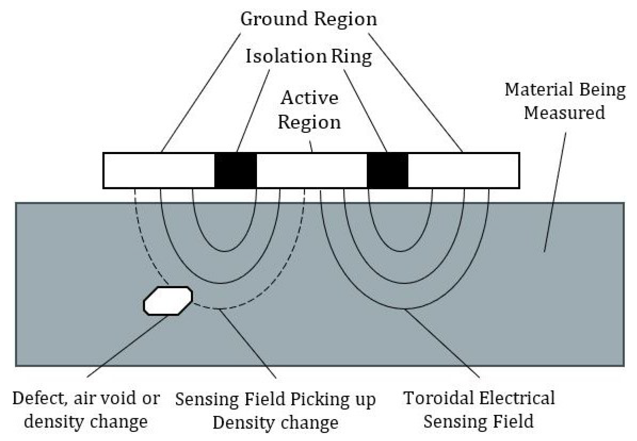
EDG operates on the principles of electromagnetic induction [16]. As illustrated in Figure 3, the sensing component of EDG comprises an active region, a ground region, and an isolation ring between them. During operation, a single-frequency voltage is applied to the active region, generating a toroidal electric sensing field over the measured asphalt pavement. Variations in the electric field occur due to internal air voids or density fluctuations within the asphalt mixture. These variations are then sensed by the ground region and converted into density measurements using the built-in algorithm [17]. EDG can also be applied to check the potential section with defects, like cracking. An internal defect may exist if an obvious density fluctuation occurs in a specific section.

However, the accuracy of EDG is not as good as NDG. This is attributed to changes in the dielectric constant of the asphalt mixture caused by temperature and moisture variations [8]. An asphalt mixture consists of aggregate and asphalt binder, with air voids typically present between them. Consequently, the asphalt mixture contains small amounts of air or even water after rainfall. Notably, the dielectric constant of water is significantly higher than that of aggregate and asphalt binder, affecting the sensitivity of the electric field variation [16]. Furthermore, the dielectric constant of water fluctuates with temperature changes. Enhancing EDG’s accuracy requires the development of a better model accounting for the effect of temperature and moisture.

3. Artificial Neural Network (ANN)

The EDG’s measurement accuracy can be improved through intelligent data-processing methods, one of which is Artificial Neural Network (ANN), the most widely used method inspired by biological neuron networks [11,18,19]. As illustrated in Figure 4, the fundamental unit of an ANN is an artificial neuron, where an ANN model computes its output. Before inputting into an artificial neuron, inputs are assigned corresponding weights. Then, the weighted sum of the inputs is calculated, and the result is fed into an activation function, which determines the neuron’s contribution [20,21]. The output of the activation function represents the final output of the neuron and is transmitted to the next neuron in the network.

3.1. Structure of the ANN Models

The artificial neurons are then organized into layers within the ANN model. As illustrated in Figure 5, the ANN comprises three layers: an input layer, two hidden layers, and an output layer. The input layer consists of 3 neurons. Since the ANN model aims to enhance the accuracy of the EDG affected by the fluctuating temperature and moisture, the inputs to the model are EDG density readings, temperature, and moisture. However, there is no computation within the input layer; instead, the input data are directly transmitted to the neurons in the hidden layers. The number of neurons in the two hidden layers is set to be the same. To explore how the number of neurons influences the accuracy of the ANN models, the range of neurons varies from 3 to 30. The minimum number of neurons typically equals or exceeds the number of input variables [21]. The number of input variables in this research is three. Hence, the minimum number is set to 3. The maximum number of neurons is determined based on the performance of the ANN models. When the number of neurons is more than 30, the performance of all ANN models obviously worsens. On the other hand, more and more storage space is required as the number of neurons increases. Thus, the maximum number of neurons is set to 30. The performance of the three ANN models is discussed in Section 5. Following computation in the hidden layers, the results are forwarded to the output layer. The output layer consists of only one neuron, and the final output from this neuron represents the ANN-predicted density.

3.2. Training Process

The training process is essential for enhancing the performance of the ANN model [22,23,24]. As shown in Figure 6, the EDG density, temperature, and moisture data are organized as three input vectors in the training process. After inputting these vectors, an ANN model with the initial weights calculates and outputs the result, which is the ANN-predicted density vector. Then, it is compared with the target density vector, which contains the NDG density data, and the resulting error vector is subsequently calculated. Finally, this error vector is utilized to adjust the weight vector of the ANN model, and a training process is done [25]. The three input vectors are inputted into the ANN model with the adjusted weights again, and a new training process runs similarly. The method of adjusting the weight vector and minimizing the error vector varies depending on the applied learning algorithms, including Levenberg-Marquardt, Bayesian regularization, and scaled conjugate gradient algorithms.

3.3. Levenberg-Marquardt (LM) Algorithm

In this study, three commonly used learning algorithms are applied to train the ANN model. The first one is the LM algorithm whose key parts involve updating the weight vector $\mathbf{w}$ and calculating the performance function $F\left(\mathbf{w}\right)$ by the following equations [12]:

$$F\left(\mathbf{w}\right)=\frac{1}{2}\sum _{i=1}^N{\mathrm{v}}_i^2\left(\mathbf{w}\right)=\frac{1}{2}{\mathbf{v}}^{\mathrm{T}}\left(\mathbf{w}\right)\mathbf{v}\left(\mathbf{w}\right)$$

(1)

$${\mathbf{w}}_{k+1}={\mathbf{w}}_k+{\mathbf{A}}_k^{-1}{\mathbf{g}}_k$$

(2)

$${\mathbf{A}}_k\approx {\mathbf{H}}_k+{\mu }_k\mathbf{I}$$

(3)

where $\mathbf{v}$ is the error vector containing all the errors ${\mathrm{v}}_i$ between the ANN-predicted density and the NDG density reading. N is the dimension of $\mathbf{v}$. ${\mathbf{w}}_k$ is the weight vector in the kth iteration step. ${\mathbf{H}}_k$ is the Hessian matrix of $F\left({\mathbf{w}}_k\right)$ and ${\mathbf{g}}_k$ is the gradient of $F\left({\mathbf{w}}_k\right)$. ${\mathbf{A}}_k$ is the approximate Hessian matrix, and its inverse matrix is used to determine the search direction with ${\mathbf{g}}_k$. $\mathbf{I}$ is an identity matrix and $\mu$ is a coefficient.

However, computing the second derivative of $F\left({\mathbf{w}}_k\right)$ to form the Hessian matrix is very computationally intensive. A simpler Jacobian matrix is introduced to approximate the Hessian matrix as well as the gradient [12,26]. The relations between them, along with the elements of the Jacobian matrix, are described by the following equations:

$${\mathbf{J}}_{ij}=\frac{\partial {\mathrm{v}}_i\left(\mathbf{w}\right)}{\partial {\mathrm{w}}_j}(i=1,\dots ,N)(j=1,\dots ,n)$$

(4)

$${\mathbf{H}}_k={\mathbf{J}}^{\mathrm{T}}\left({\mathbf{w}}_{\mathbf{k}}\right)\mathbf{J}\left({\mathbf{w}}_{\mathbf{k}}\right)$$

(5)

$${\mathbf{g}}_k={\mathbf{J}}^{\mathrm{T}}\left({\mathbf{w}}_{\mathbf{k}}\right)\mathbf{v}\left({\mathbf{w}}_{\mathbf{k}}\right)$$

(6)

$${\mathbf{w}}_{k+1}={\mathbf{w}}_k-{({\mathbf{J}}^{\mathrm{T}}\left({\mathbf{w}}_{\mathbf{k}}\right)\mathbf{J}\left({\mathbf{w}}_{\mathbf{k}}\right)+{\mu }_k\mathbf{I})}^{-1}{\mathbf{J}}^{\mathrm{T}}\left({\mathbf{w}}_{\mathbf{k}}\right)\mathbf{v}\left({\mathbf{w}}_{\mathbf{k}}\right)$$

(7)

3.4. Bayesian Regularization (BR) Algorithm

Derived from the LM algorithm, the BR algorithm is designed to mitigate the overfitting issue and enhance the generalization capability of the ANN model [13]. Unlike the LM algorithm, which focuses solely on optimizing the performance function, the BR algorithm aims to balance the performance function and the total sum of squared weights through the following equations:

$$F_{ob}\left(\mathbf{w}\right)=\beta F\left(\mathbf{w}\right)+\alpha S\left(\mathbf{w}\right)=\beta \sum _{i=1}^N{\mathrm{v}}_i^2\left(\mathbf{w}\right)+\alpha \sum _{i=1}^n{\mathrm{w}}_i^2$$

(8)

$$\mathbf{A}=2\beta {\mathbf{J}}^{\mathrm{T}}\left(\mathbf{w}\right)\mathbf{J}\left(\mathbf{w}\right)+2\alpha \mathbf{I}$$

(9)

$$\alpha =\frac{\gamma }{2S\left(\mathbf{w}\right)}$$

(10)

$$\beta =\frac{N-\gamma }{2F\left(\mathbf{w}\right)}$$

(11)

$$\gamma =N-2\alpha \mathrm{tr}{\left(\mathbf{A}\right)}^{-1}$$

(12)

where $F_{ob}\left(\mathbf{w}\right)$ is the objective function required to be optimized. $S\left(\mathbf{w}\right)$ is the total sum of squared weights. $\alpha$, $\beta$, and $\gamma$ are the three coefficients to balance $S\left(\mathbf{w}\right)$ and $F\left(\mathbf{w}\right)$. $\mathrm{tr}\left(\mathbf{A}\right)$ is the trace of $\mathbf{A}$.

In the BR algorithm, both the equations in this subsection and Section 3.3 are used. Firstly, the coefficients $\alpha$ and $\beta$ are set randomly, the coefficients $\gamma$ is set as N. Secondly, $F\left(\mathbf{w}\right)$, $S\left(\mathbf{w}\right)$ and $F_{ob}\left(\mathbf{w}\right)$ are calculated through Equation (8). Thirdly, $\mathbf{J}$, $\mathbf{g}$ and $\mathbf{A}$ are calculated through Equations (4), (6) and (9), respectively. Fourthly, the weight vector $\mathbf{w}$ is updated through Equation (2). Fifthly, the coefficients $\alpha$, $\beta$, and $\gamma$ are updated through Equations (10)–(12). Finally, the steps mentioned above are repeated until the optimized weights and errors are calculated.

Compared to the LM-ANN model, the BR-ANN model generally exhibits superior generalization capability, indicating similar performance on both the training and test data sets. However, due to the increased complexity involved in calculating both $F\left(\mathbf{w}\right)$ and $S\left(\mathbf{w}\right)$ parts and the extra 3 coefficients, the training time of the BR-ANN model tends to be longer than that of the LM-ANN model.

3.5. Scaled Conjugate Gradient (SCG) Algorithm

Unlike the LM algorithm, which relies on the Jacobian matrix, the SCG algorithm determines the search direction using a series of conjugate vectors [14]. The conjugate and weight vector are updated according to the following equations:

$${\mathbf{w}}_{k+1}={\mathbf{w}}_k+c_k{\mathbf{p}}_k$$

(13)

$${\mathbf{p}}_k=-{\mathbf{g}}_k+{\lambda }_k{\mathbf{p}}_{k-1}$$

(14)

$${\lambda }_k=\frac{\Delta {\mathbf{g}}_{k-1}^{\mathrm{T}}{\mathbf{g}}_k}{\Delta {\mathbf{g}}_{k-1}^{\mathrm{T}}{\mathbf{p}}_{k-1}}$$

(15)

where $\mathbf{p}$ is the conjugate vector. c and $\lambda$ are two coefficients to support establishing the conjugate vector and training the model.

Compared with the other two models, the SCG-ANN model requires the shortest training time. This is because operations on conjugate vectors are less computationally intensive than on Jacobian matrices. Additionally, the model is less prone to the overfitting issue, leading to a better generalization capability. However, this also implies that the model’s accuracy may be compromised.

3.6. Collected Data and Input Data

In addition to the learning algorithms, the collected data are also important for the ANN training process. A total of 290 data samples were collected with the support of Fulton Hogan technicians. Before the measurements, the entire asphalt pavement was divided into 29 engineering lots. Approximately 10 locations (ranging from 8 to 11 locations depending on the lot) were randomly selected in each lot, with one location selected per 300 m². These selected locations were marked for reference. The NDG and EDG were then set up and calibrated according to the properties of the pavement materials and were put on the same locations to get the density readings. Additionally, the EDG could also measure temperature and moisture at the same time.

The collected data samples are separated into three types of input data: training, validation, and test input data (comprising 60%, 20%, and 20% of the data, respectively). The training data are directly utilized to train the ANN models. The validation data are employed to validate the performance of the models during the training process and to promptly halt the process to prevent potential overfitting issues, which could lead to poor generalization capability. The test data are not utilized for training the model; instead, they are considered as new data to test and evaluate the performance of the models. How to apply the distinct performances of a model with three types of input data in this approach is discussed in the next section.

4. Methodology

The proposed ANN approach includes the optimization of the ANN structure and the evaluation of the optimized models. The optimization process starts with the ANN model having 3 neurons in its hidden layer. Subsequently, the number of neurons increases by 1 in each step until it reaches 30. The ANN model is trained 100 times at each step, and the average performance is recorded. The performances of an ANN model is mainly indicated by the root mean squared error (RMSE) between the ANN-predicted density and the NDG density reading:

$$RMSE=\sqrt{\frac{{\Sigma }_{i=1}^{\mathrm{n}}{(X_i-Y_i)}^2}{\mathrm{n}}}$$

(16)

where X and Y are the NDG density reading and ANN-predicted density, respectively. n is the total number of densities.

Another performance index is the correlation coefficients (R values):

$$R=\frac{{\Sigma }_{i=1}^{\mathrm{n}}(X_i-\overline{X})(Y_i-\overline{Y})}{\sqrt{{\Sigma }_{i=1}^{\mathrm{n}}{(X_i-\overline{X})}^2{(Y_i-\overline{Y})}^2}}$$

(17)

where $X_i$ and $Y_i$ are the NDG density reading and ANN-predicted density, respectively. $\overline{X}$ and $\overline{Y}$ are the average values of $X_i$ and $Y_i$, respectively. n is the total number of densities.

In detail, the optimization and evaluation of the ANN models proceed in the following manner: Firstly, the average accuracy of the models is assessed by comparing the RMSEs of the three models with the corresponding training and test data. The RMSE of the model with the test data is particularly significant in determining the accuracy, although that of the one with the training data is also considered. Secondly, the average generalization capability of the models is evaluated based on two conditions. The first condition is whether the RMSE of the model with the test or validation data continuously increases as the number of neurons grows. The second condition is whether the two differences continuously increase as the number of neurons grows. The two differences refer to the difference between the RMSEs of the model with the training and test data, as well as the difference between the RMSEs of the same model with the training and validation data. Thirdly, the average training time of each model is analyzed. Finally, the optimized LM-ANN, BR-ANN, and SCG-ANN models are selected based on the aforementioned optimizations and evaluations. Their performances are determined by both their RMSEs and their R values.

5. Results and Discussion

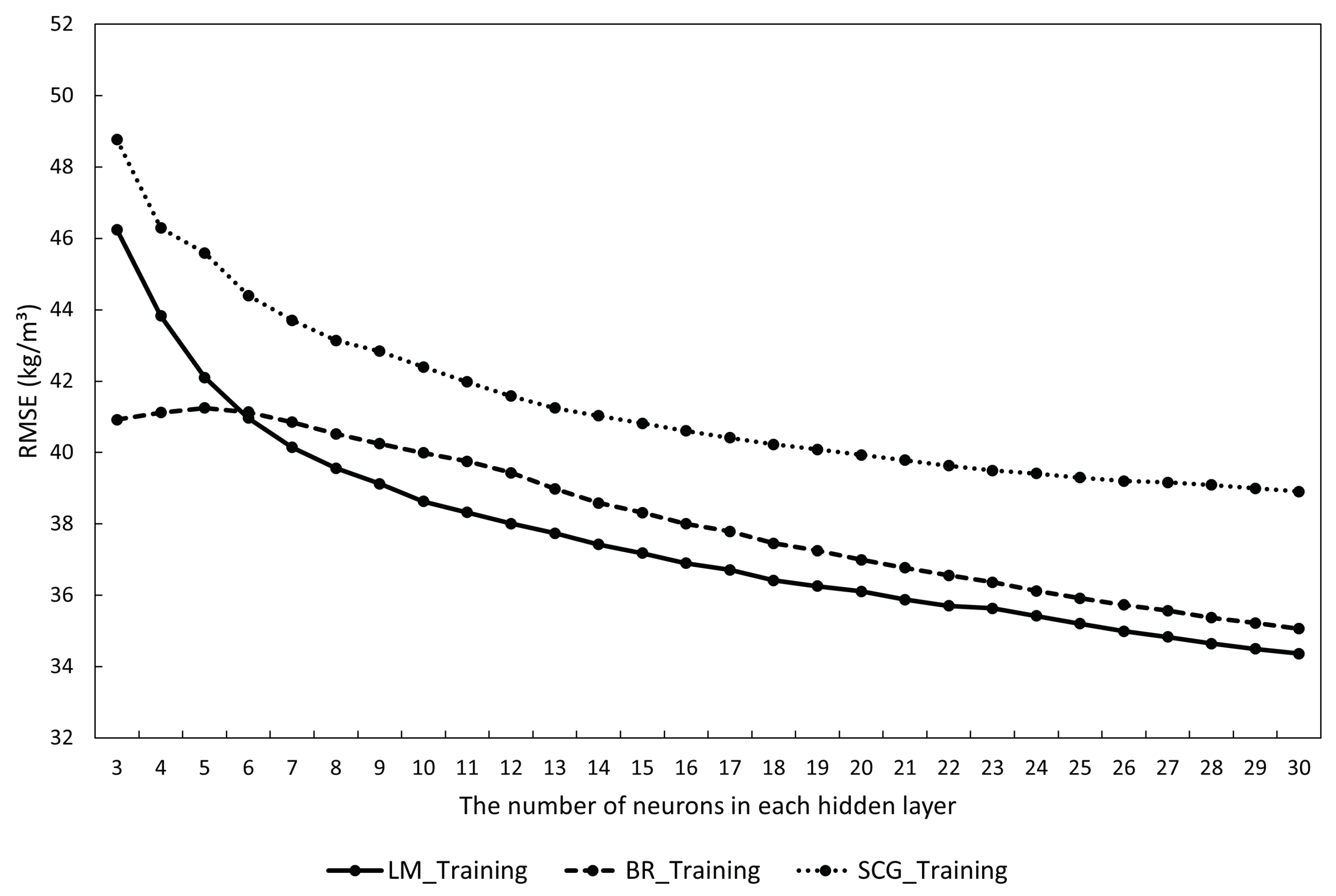
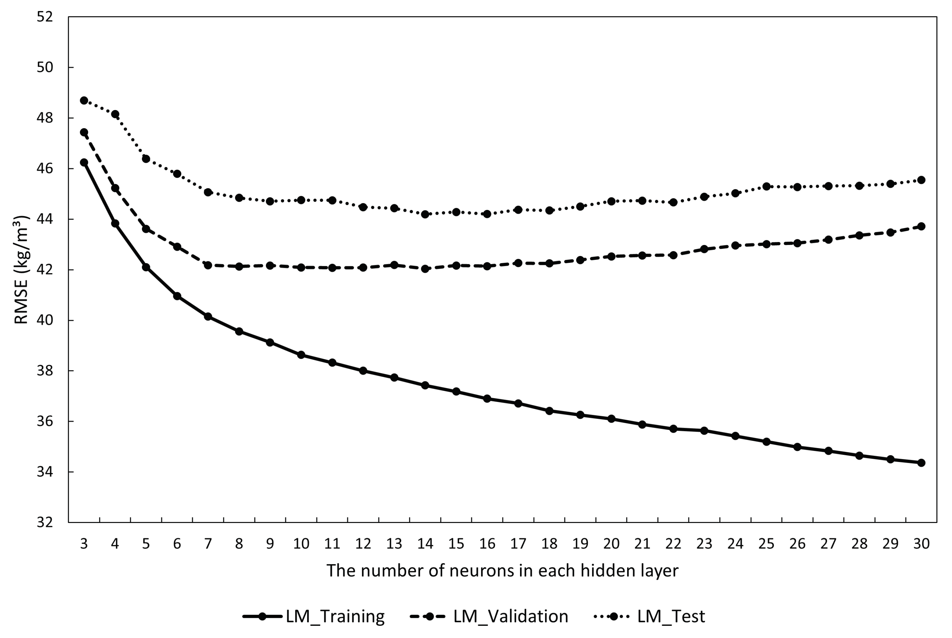
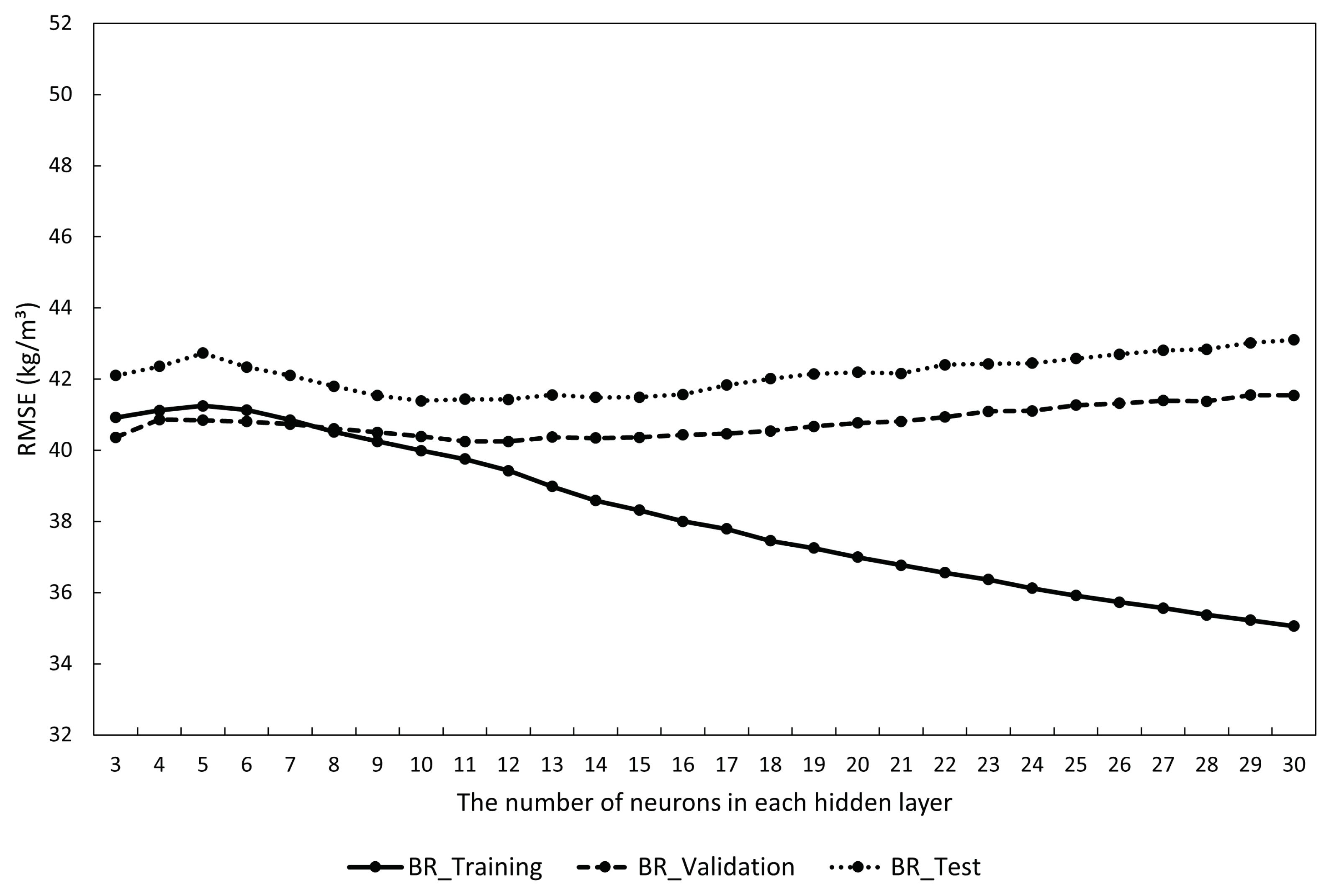
The average performances of the three models with different numbers of neurons are illustrated in

Table 1. The average performance of the LM-ANN model.

The Number of Neurons in Each Hidden Layer	LM-ANN Model
	Training Time (s)	RMSE (kg/m3)
		Training	Validation	Test
3	0.086	46.25	47.44	48.70
4	0.078	43.83	45.23	48.16
5	0.078	42.10	43.62	46.38
6	0.075	40.96	42.91	45.79
7	0.075	40.14	42.18	45.06
8	0.076	39.56	42.13	44.84
9	0.077	39.12	42.17	44.71
10	0.077	38.63	42.09	44.75
11	0.079	38.32	42.07	44.75
12	0.080	38.00	42.09	44.48
13	0.081	37.73	42.19	44.43
14	0.082	37.42	42.04	44.19
15	0.085	37.18	42.17	44.29
16	0.087	36.90	42.14	44.20
17	0.092	36.71	42.26	44.37
18	0.098	36.42	42.25	44.34
19	0.104	36.26	42.39	44.50
20	0.111	36.10	42.53	44.71
21	0.123	35.88	42.57	44.73
22	0.130	35.71	42.58	44.66
23	0.141	35.63	42.81	44.89
24	0.152	35.42	42.96	45.02
25	0.169	35.20	43.01	45.29
26	0.184	34.99	43.05	45.27
27	0.204	34.83	43.19	45.31
28	0.224	34.65	43.36	45.32
29	0.250	34.50	43.48	45.39
30	0.279	34.36	43.71	45.55

,

Table 2. The average performance of the BR-ANN model.

The Number of Neurons in Each Hidden Layer	BR-ANN Model
	Training Time (s)	RMSE (kg/m3)
		Training	Validation	Test
3	0.095	40.92	40.36	42.10
4	0.092	41.12	40.87	42.36
5	0.093	41.25	40.84	42.73
6	0.093	41.13	40.80	42.34
7	0.094	40.85	40.73	42.10
8	0.097	40.52	40.61	41.80
9	0.098	40.25	40.50	41.54
10	0.100	39.99	40.39	41.39
11	0.102	39.75	40.25	41.43
12	0.103	39.43	40.25	41.43
13	0.105	38.98	40.37	41.56
14	0.108	38.59	40.34	41.49
15	0.113	38.32	40.36	41.49
16	0.116	38.00	40.43	41.57
17	0.123	37.79	40.47	41.84
18	0.132	37.46	40.54	42.01
19	0.143	37.25	40.67	42.15
20	0.154	37.00	40.77	42.19
21	0.170	36.77	40.81	42.16
22	0.183	36.56	40.94	42.41
23	0.200	36.37	41.09	42.43
24	0.223	36.12	41.11	42.45
25	0.248	35.92	41.27	42.58
26	0.277	35.73	41.32	42.70
27	0.310	35.57	41.40	42.81
28	0.346	35.37	41.37	42.84
29	0.388	35.22	41.55	43.02
30	0.447	35.06	41.54	43.10

and

Table 3. The average performance of the SCG-ANN model.

The Number of Neurons in Each Hidden Layer	SCG-ANN Model
	Training Time (s)	RMSE (kg/m3)
		Training	Validation	Test
3	0.070	48.77	47.61	50.32
4	0.068	46.29	45.28	47.95
5	0.067	45.59	44.61	47.36
6	0.067	44.40	43.85	46.03
7	0.066	43.70	43.35	45.73
8	0.066	43.14	43.01	45.28
9	0.066	42.84	42.61	44.96
10	0.066	42.39	42.30	44.58
11	0.066	41.98	41.94	44.04
12	0.066	41.58	41.74	43.82
13	0.066	41.25	41.57	43.61
14	0.067	41.03	41.39	43.58
15	0.067	40.81	41.36	43.45
16	0.067	40.61	41.38	43.39
17	0.067	40.41	41.34	43.32
18	0.067	40.23	41.27	43.22
19	0.068	40.09	41.37	43.35
20	0.068	39.93	41.38	43.41
21	0.068	39.78	41.52	43.51
22	0.068	39.63	41.59	43.62
23	0.069	39.50	41.59	43.68
24	0.069	39.41	41.75	43.90
25	0.070	39.30	41.85	43.97
26	0.070	39.20	41.92	43.98
27	0.070	39.16	41.98	44.08
28	0.070	39.09	42.04	44.20
29	0.071	39.00	42.23	44.46
30	0.071	38.90	42.32	44.52

and Figure 7, Figure 8, Figure 9, Figure 10, Figure 11 and Figure 12. These figures are made based on the results in those tables to better describe the accuracy, generalization capability, and training time of the three models, respectively.

5.1. The Average Accuracy of the Three Models

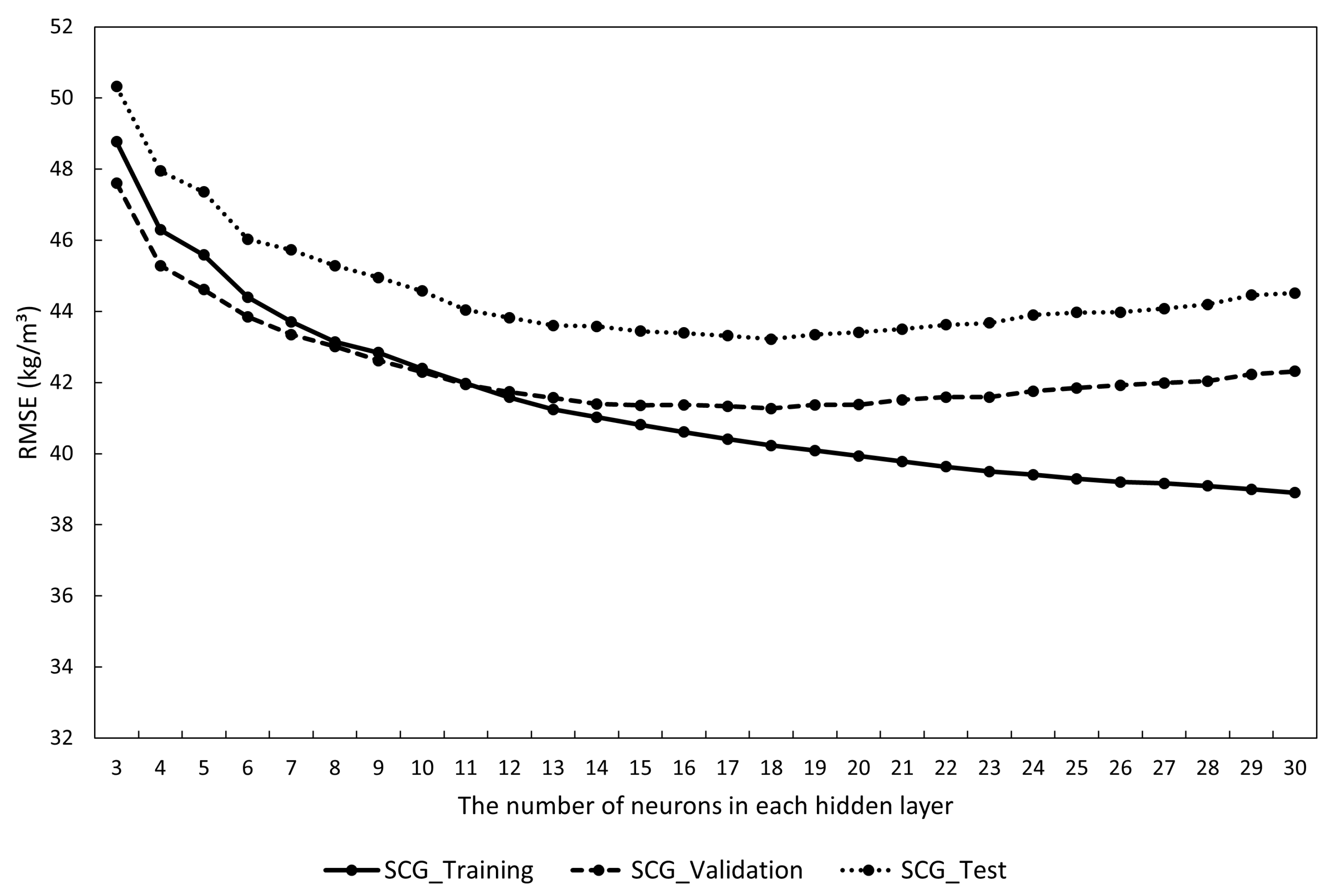
Firstly, the average accuracy of the three ANN models is analyzed. The RMSEs of them with the corresponding training data are depicted in Figure 7. In terms of the LM-ANN model, the RMSE is 46.25 kg/m³ at the beginning of the optimization. It gradually decreases to 39.12 kg/m³ as the number of neurons increases to 9. Subsequently, it decreases gradually at a lower rate, reaching 34.36 kg/m³ by the end of the optimization. Regarding the BR-ANN model, the RMSE is 40.92 kg/m³ at the start of the optimization. It initially increases to 41.25 kg/m³ as the number of neurons grows to 5, then begins to decline, reaching 39.43 kg/m³ as the number goes up to 12. Eventually, it decreases at a similar rate as the RMSE of the LM-ANN model, reaching 35.06 kg/m³ when the optimization goes to the end. As for the SCG-ANN model, the RMSE is 48.77 kg/m³ when the optimization begins. It reduces to 41.25 kg/m³ as the number of neurons rises to 13. Subsequently, it continues to decline steadily at lower rates (less than 0.22 kg/m³ per neuron), reaching 39.78 kg/m³ when the number of neurons is 21. Finally, it decreases at lower rates (less than 0.15 kg/m³ per neuron) to 38.90 kg/m³ when the model contains 30 neurons in each hidden layer. Comparing the three models, the RMSE of the SCG-ANN model is consistently the largest throughout the optimization process. The gap between it and that of the LM-ANN model is approximately 2.5 kg/m³ when the number of neurons is less than 4. However, this gap ranges between 3.43 and 4.54 kg/m³ when the number exceeds 5. Conversely, the RMSE of the BR-ANN model is the smallest if the number of neurons is less than 6. There is a minor gap (ranging from 0.70 to 1.43 kg/m³) between those of the LM-ANN and the BR-ANN model when the number exceeds 6.

The RMSEs of the three models with the corresponding test data are illustrated in Figure 8. When the optimization begins, the RMSE of the LM-ANN model is 48.70 kg/m³. It slumps to 44.71 kg/m³ as the number of neurons increases to 9. Subsequently, it stabilizes briefly before experiencing a slight decrease to 44.19 kg/m³ as the number goes up to 14. Finally, it creeps up to 45.55 kg/m³ by the end of the optimization. In terms of the BR-ANN model, the RMSE gradually increases from 42.10 to 42.73 kg/m³ as the number of neurons rises from 3 to 5. It then slightly decreases to 41.39 kg/m³ as the number climbs to 10 and fluctuates between 41.43 and 41.57 kg/m³ as the number varies from 11 to 16. Lastly, it continues to rise to 43.10 kg/m³ as the optimization goes to the end. As for the SCG-ANN model, the RMSE dives from 50.32 to 43.82 kg/m³ as the number of neurons rises from 3 to 12. It then decreases at the rates around 0.1 kg/m³ per neuron to 43.22 kg/m³ as the number of neurons rises from 12 to 18. Eventually, it gradually grows to 44.52 kg/m³ as the number goes up to 30. Comparing the three models, the RMSE of the LM-ANN model is initially smaller than that of the SCG-ANN model, with a gap of approximately 1.6 kg/m³. However, if the number of neurons exceeds 10, the RMSE of the LM-ANN model surpasses that of the SCG-ANN model, with the increasing gap to 1.03 kg/m³ by the end of optimization. Conversely, the RMSE of the BR-ANN model is the smallest among the three RMSEs. The difference between those of the LM-ANN and BR-ANN models decreases from approximately 6.6 to 3.0 kg/m³, then slightly increases to 3.4 kg/m³ as the number of neurons increases from 3 to 10. Finally, it gradually decreases to 2.45 kg/m³ as the optimization goes to the end.

In summary, the two figures illustrate the totally different results. In the first figure, the RMSE of the LM-ANN model with the training data is the smallest when the number of neurons is more than 6. The reason is that the LM algorithm can optimize the weights of the ANN model by calculating the approximate Hessian matrix. The matrix contains enough information to improve the possibility of reaching the optimal search direction during the training process. Thus, the LM-ANN model has a good accuracy. The RMSE of the BR-ANN model is larger than the former one since the accuracy of the BR-ANN model is reduced to improve the generalization capability. The RMSE of the SCG-ANN model is the largest among the three RMSEs. The reason is that the conjugate vectors contain less information than the approximate Hessian matrix. Hence, reaching the optimal search direction is harder, resulting in a worse performance of the SCG-ANN model. In the second figure, the RMSE of the BR-ANN model with the test data is the smallest. The RMSE of the SCG-ANN model is smaller than that of the LM-ANN model when the number of neurons is larger than 10. Since the test data are not used to train the ANN models, these results are affected by both of the accuracy and the generalization capability of the ANN models. The latter performance of the models is discussed in the next subsection.

5.2. The Average Generalization Capability of the Three Models

Secondly, the generalization capability of the three models is evaluated. That of the LM-ANN model with three types of input data is depicted in Figure 9. At the start of the optimization, the difference between the RMSEs of the model with training or validation data is minimal (approximately 1.2 kg/m³). This difference creeps up to around 3 kg/m³ as the number of neurons rises to 9. After that, it increases rapidly, reaching 9.35 kg/m³ eventually. This phenomenon occurs since the RMSE of the model with the training data is decreasing while that of the one with the validation data is increasing during this period. The difference between the RMSEs of the model with the training or test data follows a similar trend. Therefore, the generalization capability of the LM-ANN model is acceptable if the number of neurons is less than 9.

The generalization capability of the BR-ANN model is demonstrated in Figure 10. If the number of neurons is less than 9, the RMSEs of the model with the training and validation data are approximately equal. However, their gap starts to widen as the number of neurons exceeds 9, reaching 6.5 kg/m³ at the end of the optimization. On the other hand, the gap between the RMSEs of the model with the test and validation data is 1.74 kg/m³ at the beginning of the optimization. The RMSE of the one with the test data then follows a similar trend to that of the one with the validation data, resulting in a consistent gap throughout the optimization process. Additionally, both two RMSEs keep increasing if the number of neurons exceeds 16. Therefore, the generalization capability of the BR-ANN model performs excellently when the number of neurons is less than 16.

The generalization capability of the SCG-ANN model is illustrated in Figure 11. When the optimization starts, the RMSE of the model with the training data exceeds that of the one with the validation data, with a gap of approximately 1.2 kg/m³. Between 9 and 13 neurons, the two RMSEs are close. However, as the number of neurons increases from 14 to 30, the RMSE of the model with validation data overtakes the one with the training data, resulting in a gap widening from around 0.4 to 3.4 kg/m³. Similarly, the RMSE of the model with the test data follows a similar trend to that of the one with the validation data, with a stable gap of 2.1 kg/m³ when the number of neurons exceeds 11. Additionally, both two RMSEs begin to creep up as the number of neurons rises to 18 or more. Overall, the generalization capability of the SCG-ANN model is excellent, good, and still acceptable when the number of neurons is in the range of 2 to 8, 9 to 18, and 19 to 30, respectively.

In summary, the generalization capability of an ANN model is highly affected by the learning algorithm. When the three ANN models hold the same number of neurons, the gap between the RMSEs of the LM-ANN model with the training and the test data is larger than that of the BR-ANN or SCG-ANN model. Thus, the LM-ANN model performs the worst generalization capability. Theoretically, the LM algorithm is designed to improve the accuracy rather than the generalization capability of the trained model. To reach the goal, the features of the training data may be over-explored. Since the test and validation data are not used in the training process, some of their features may be ignored. Hence, the LM-ANN model with the test or validation data performs worse than the LM-ANN model with training data. Conversely, the BR algorithm can enhance the generalization capability by balancing the performance function and the total sum of squared weights. Commonly, a true model holds a smooth surface. One way to make the surface smoother is to reduce the coefficients of the model. In an ANN model, a similar way is to reduce the weights. Hence, reducing the total sum of squared weights commonly makes the ANN model close to the true model, resulting in an excellent generalization capability. Furthermore, the SCG-ANN model also holds a good generalization capability. Compared with the approximate Hessian matrix, the conjugate vectors contain less information of the performance function. Although the features of the training data can still be over-explored, the possibility becomes less.

5.3. The Average Training Time of the Three Models

Thirdly, the training time of the three models, described in Figure 12, is analyzed. At the beginning of optimization, the training time of the LM-ANN model is 0.086 s. It decreases to 0.075 s as the number of neurons increases to 6, then rises to 0.082 s as the number goes up to 14 neurons. Subsequently, its growth rate accelerates, reaching 0.279 s by the end of optimization. For the BR-ANN model, the training time remains slightly less than 0.1 s if the number of neurons ranges from 3 to 10, then it increases to 0.108 s when the number of neurons reaches 14. Following a similar trend to the LM-ANN model but with a higher growth rate, it reaches 0.447 s at the end of optimization. As for the SCG-ANN model, its training time decreases slightly from 0.070 to 0.066 s, then remains constant, and finally, increases back to 0.071 s as the number of neurons grows from 3 to 7, from 8 to 13, and from 14 to 30. Overall, establishing an ANN model with too many neurons in its hidden layer is not efficient, except for the SCG-ANN model.

In summary, the training time of the SCG-ANN model is the shortest since the least computation is required in the training process. On the contrary, the training time of the BR-ANN model is the longest since both the approximate Hessian matrix and the additional coefficients parts are required to be calculated.

5.4. The Performances of the Optimized Models

Ultimately, the optimized models are selected based on the aforementioned analysis, and their performances are evaluated. The two optimized LM-ANN models are the ones with 9 and 14 neurons in each hidden layer. The performances of the two optimized models are illustrated in

Table 4. The performance of the optimized LM-ANN models.

The Number of Neurons in Each Hidden Layer	LM-ANN Models
	R Value			RMSE (kg/m3)
	Training	Validation	Test	Training	Validation	Test
9	0.943	0.923	0.924	37.61	41.73	43.32
14	0.953	0.942	0.916	34.25	40.61	41.54

. As for the first model, the R value of the model with the training data is higher than that of the model with the validation or test data (0.943 compared with 0.923 or 0.924, respectively). The RMSE of the model with the training data is the smallest, while that of the model with the test data is the greatest (37.61 kg/m³ compared with 43.32 kg/m³). Moreover, that of the model with the validation data is 41.73 kg/m³. Regarding the second model, the R value of the model with the training data is the highest, followed by that of the model with the validation data (0.953 and 0.942, respectively). The R value of the model with the test data is 0.916, which is acceptable. On the other hand, the RMSE of the model with the test data is the greatest, while that of the one with the training data is the smallest (41.54 compared with 34.25 kg/m³). That of the one with the validation data is 40.61 kg/m³. Comparing the two optimized models, the performance of the LM-ANN model improves as the number of neurons rises from 9 to 14. However, the RMSEs of the models with the corresponding validation and test data are all more than 40 kg/m³. Hence, none of the LM-ANN models is sufficiently accurate.

The three optimized BR-ANN models hold 5, 10, and 16 neurons in each hidden layer, respectively. The performances of the three optimized models are demonstrated in

Table 5. The performance of the optimized BR-ANN models.

The Number of Neurons in Each Hidden Layer	BR-ANN Models
	R Value			RMSE (kg/m3)
	Training	Validation	Test	Training	Validation	Test
5	0.938	0.930	0.945	38.26	36.06	39.42
10	0.937	0.912	0.954	38.52	37.95	37.82
16	0.947	0.945	0.919	36.41	38.55	37.52

. Regarding the first model, its three R values range from 0.930 to 0.945. The RMSE of the model with the validation data is acceptable, while the RMSEs of it with the training and test data are great (36.06 compared with 38.26 and 39.42 kg/m³). As for the second model, the R values of the model with the training and test data are reasonable, and that of it with the validation data is acceptable (0.937, 0.954, and 0.912). Its three RMSEs are 38.52, 37.95, and 37.82 kg/m³, respectively. Since the RMSE of the model with the validation or test data is smaller than that of it with the training data, the generalization capability of it is considered good. In terms of the third model, the R values of the model with the training and validation data are good and approximately the same (0.947 and 0.945, respectively). Even if the R value of the model with the test data, which is the lowest (0.919), is still sufficient. Similarly, although the RMSE of the model with the validation or test data is slightly higher than that of the model with the training data, they are still acceptable (38.55 and 37.52 compared with 36.41 kg/m³). Overall, both the performances of the second and third BR-ANN models are acceptable. The generalization capability of the former one is better, while the accuracy of the latter one is higher.

The three optimized SCG-ANN models contain 8, 14, and 18 neurons in each hidden layer, respectively. The performances of the three optimized models are illustrated in

Table 6. The performance of the optimized SCG-ANN models.

The Number of Neurons in Each Hidden Layer	SCG-ANN Models
	R Value			RMSE (kg/m3)
	Training	Validation	Test	Training	Validation	Test
8	0.928	0.930	0.951	41.44	39.86	37.08
14	0.948	0.947	0.931	36.81	35.33	34.97
18	0.947	0.940	0.952	35.17	36.86	38.11

. In terms of the first model, the R value of the model with the test data is 0.951, which is excellent. Additionally, the other two R values are reasonable and similar (0.928 and 0.930, respectively). However, all three RMSEs of it are relatively large (41.44, 39.86, and 37.08 kg/m³, respectively). As for the second model, the R values of the model with the training and validation data are excellent and roughly the same (0.948 and 0.947, respectively). The last R value is 0.931, which is also reasonable. Moreover, its three RMSEs are 36.81, 35.33, and 34.97 kg/m³, which are relatively small. Hence, both the accuracy and generalization capability of the second model are outstanding. Regarding the third model, its three R values are 0.947, 0.940, and 0.952, which are all excellent. The RMSEs of it with the training and validation data are 35.17 and 36.86 kg/m³, which are acceptable. Nevertheless, the last RMSE is 38.11 kg/m³, which is slightly large but acceptable. Overall, the performance of the second model is excellent, and that of the third is also good.

Overall, the four sufficient models include the last two BR-ANN models and SCG-ANN models. Their performances are then compared with the original performance of the EDG. The R value and the RMSE of the original EDG density readings are 0.920 and 44.86 kg/m³, respectively. As for the second BR-ANN model, although the R value of the model with the validation data is lower than 0.920, that of the model with the training or test data is much higher than 0.920. In addition, the three RMSEs are all smaller than 44.86 kg/m³. Hence, the overall performance of this model is better than the original performance. Similarly, in terms of the third BR-ANN model, the R value of the model with the test data is slightly lower than 0.920, while the other R values are significantly higher than 0.920. Moreover, its three RMSEs also perform better. Thus, the overall performance of this model is also better. Regarding the two SCG-ANN models, their performances are obviously excellent.

In summary, the two LM-ANN models are considered inappropriate. Conversely, the last two BR-ANN and SCG-ANN models have reliable accuracy and generalization capability and can be utilized to improve the performance of the EDG measurement.

6. Conclusions

EDG and NDG are the two devices commonly used in the non-destructive measurement of asphalt pavement density. However, the accuracy of EDG is lower than that of NDG since the former one is affected by temperature and moisture. This paper presents an ANN approach to enhance the accuracy of EDG. The EDG density, temperature and moisture are the three input variables for training the ANN models. The NDG density is regarded as the target density. Three learning algorithms are used in the training process, including the LM, BR, and SCG algorithms. The accuracy of the LM-ANN model is the best when the training data are input. Furthermore, the generalization capability of the BR-ANN model is the best and the training time of the SCG-ANN model is the shortest. The performance of the optimized ANN model is then analyzed. The optimized LM-ANN model is not sufficiently accurate. Nevertheless, totally four BR-ANN and SCG-ANN models provide acceptable performance and all of them can greatly improve the original performance of the EDG.

References

1. Li, M.; Huang, L.; Al-Jumaily, A. Methods for Asphalt Road Density Measurement: A Review. In Proceedings of the 2021 27th International Conference on Mechatronics and Machine Vision in Practice (M2VIP), Shanghai, China, 26–28 November 2021; pp. 269–274. [Google Scholar] [CrossRef]
2. AS/NZS 2891.1.2; Methods of Sampling and Testing Asphalt—Method 1.2: Sampling—Coring Method. Standards New Zealand: Wellington, New Zealand, 2020.
3. AS/NZS 2891.9.1; Methods of Sampling and Testing Asphalt—Method 9.1: Determination of Bulk Density of Compacted Asphalt—Waxing Procedure. Standards New Zealand: Wellington, New Zealand, 2022.
4. AS/NZS 2891.9.2; Methods of Sampling and Testing Asphalt—Part 9.2: Determination of Bulk Density of Compacted Asphalt—Presaturation Method. Standards New Zealand: Wellington, New Zealand, 2022.
5. ASTM D2726/D2726M; Standard Test Method for Bulk Specific Gravity and Density of Non-Absorptive Compacted Asphalt Mixtures. American Society for Testing and Materials (ASTM): West Conshohocken, PA, USA, 2019.
6. ASTM D2950/D2950M; Standard Test Method for Density of Asphalt Mixtures in Place by Nuclear Methods. American Society for Testing and Materials (ASTM): West Conshohocken, PA, USA, 2022.
7. AASHTO T355; Standard Method of Test for In-Place Density of Asphalt Mixtures by Nuclear Methods. American Association of State Highway and Transportation Officials (AASHTO): Washington, DC, USA, 2022.
8. ASTM D7113/D7113M; Standard Test Method for Density of Bituminous Paving Mixtures in Place by the Electromagnetic Surface Contact Methods. American Society for Testing and Materials (ASTM): West Conshohocken, PA, USA, 2020.
9. AASHTO T343; Standard Method of Test for Density of In-Place Hot Mix Asphalt (HMA) Pavement by Electronic Surface Contact Devices. American Association of State Highway and Transportation Officials (AASHTO): Washington, DC, USA, 2020.
10. Helal, J.; Sofi, M.; Mendis, P. Non-Destructive Testing of Concrete: A Review of Methods. Electron. J. Struct. Eng. 2015, 14, 97–105. [Google Scholar] [CrossRef]
11. Abdolrasol, M.G.M.; Hussain, S.M.S.; Ustun, T.S.; Sarker, M.R.; Hannan, M.A.; Mohamed, R.; Ali, J.A.; Mekhilef, S.; Milad, A. Artificial Neural Networks Based Optimization Techniques: A Review. Electronics 2021, 10, 2698. [Google Scholar] [CrossRef]
12. Rubio, J.d.J. Stability Analysis of the Modified Levenberg–Marquardt Algorithm for the Artificial Neural Network Training. IEEE Trans. Neural Netw. Learn. Syst. 2021, 32, 3510–3524. [Google Scholar] [CrossRef] [PubMed]
13. Sariev, E.; Germano, G. Bayesian regularized artificial neural networks for the estimation of the probability of default. Quant. Financ. 2020, 20, 311–328. [Google Scholar] [CrossRef]
14. Yuan, G.; Li, T.; Hu, W. A conjugate gradient algorithm for large-scale nonlinear equations and image restoration problems. Appl. Numer. Math. 2020, 147, 129–141. [Google Scholar] [CrossRef]
15. Yan, Z.; Zhong, S.; Lin, L.; Cui, Z. Adaptive Levenberg–Marquardt Algorithm: A New Optimization Strategy for Levenberg–Marquardt Neural Networks. Mathematics 2021, 9, 2176. [Google Scholar] [CrossRef]
16. Wang, B.; Zhong, S.; Lee, T.L.; Fancey, K.S.; Mi, J. Non-destructive testing and evaluation of composite materials/structures: A state-of-the-art review. Adv. Mech. Eng. 2020, 12, 1687814020913761. [Google Scholar] [CrossRef]
17. Gupta, M.; Khan, M.A.; Butola, R.; Singari, M. Advances in applications of Non-Destructive Testing (NDT): A review. Adv. Mater. Process. Technol. 2022, 8, 2286–2307. [Google Scholar] [CrossRef]
18. Liu, X.; Tian, S.; Tao, F.; Yu, W. A review of artificial neural networks in the constitutive modeling of composite materials. Compos. Part Eng. 2021, 224, 109152. [Google Scholar] [CrossRef]
19. Mumali, F. Artificial neural network-based decision support systems in manufacturing processes: A systematic literature review. Comput. Ind. Eng. 2022, 165, 107964. [Google Scholar] [CrossRef]
20. Chen, Y.; Song, L.; Liu, Y.; Yang, L.; Li, D. A Review of the Artificial Neural Network Models for Water Quality Prediction. Appl. Sci. 2020, 10, 5776. [Google Scholar] [CrossRef]
21. Grum, M.; Gronau, N.; Heine, M.; Timm, I. Construction of a Concept of Neuronal Modeling; Springer Gabler: Wiesbaden, Germany, 2020. [Google Scholar]
22. Kaloev, M.; Krastev, G. Comprehensive Review of Benefits from the Use of Neuron Connection Pruning Techniques During the Training Process of Artificial Neural Networks in Reinforcement Learning: Experimental Simulations in Atari Games. In Proceedings of the 2023 7th International Symposium on Multidisciplinary Studies and Innovative Technologies (ISMSIT), Ankara, Turkiye, 26–28 October 2023. [Google Scholar] [CrossRef]
23. Kim, S. Improving ANN Training with Approximation Techniques for ROCOF Trajectory Estimation. In Proceedings of the 2023 IEEE Belgrade PowerTech, Belgrade, Serbia, 25–29 June 2023; pp. 1–6. [Google Scholar]
24. Krajinski, P.; Sourkounis, C. Training of an ANN Feed-Forward Regression Model to Predict Wind Farm Power Production for the Purpose of Active Wake Control. In Proceedings of the 2022 IEEE 21st Mediterranean Electrotechnical Conference (MELECON), Palermo, Italy, 14–16 June 2022; pp. 954–959. [Google Scholar]
25. Tuan Hoang, A.; Nižetić, S.; Chyuan Ong, H.; Tarelko, W.; Viet Pham, V.; Hieu Le, T.; Quang Chau, M.; Phuong Nguyen, X. A review on application of artificial neural network (ANN) for performance and emission characteristics of diesel engine fueled with biodiesel-based fuels. Sustain. Energy Technol. Assess. 2021, 47, 101416. [Google Scholar] [CrossRef]
26. Khakhar, P.; Dubey, R.K. Chapter 5—The integrity of machine learning algorithms against software defect prediction. In Artificial Intelligence and Machine Learning for EDGE Computing; Pandey, R., Khatri, S.K., Kumar Singh, N., Verma, P., Eds.; Academic Press: Cambridge, MA, USA, 2022; pp. 65–74. [Google Scholar] [CrossRef]
Figure 1. An NDG placed on the surface of the asphalt pavement.
Metrology 04 00019 g001
Figure 2. An EDG placed on the surface of the asphalt pavement.
Metrology 04 00019 g002
Figure 3. The working principle of EDG.
Metrology 04 00019 g003
Figure 4. An artificial neuron in the ANN model.
Metrology 04 00019 g004
Figure 5. The structure of the ANN model.
Metrology 04 00019 g005
Figure 6. The training process of the ANN model.
Metrology 04 00019 g006
Figure 7. The RMSEs of the three models with the corresponding training data.
Metrology 04 00019 g007
Figure 8. The RMSEs of the three models with the corresponding test data.
Metrology 04 00019 g008
Figure 9. The generalization capability of the LM-ANN model indicated by the RMSEs.
Metrology 04 00019 g009
Figure 10. The generalization capability of the BR-ANN model indicated by the RMSEs.
Metrology 04 00019 g010
Figure 11. The generalization capability of the SCG-ANN model indicated by the RMSEs.
Metrology 04 00019 g011
Figure 12. The training time of the three models.
Metrology 04 00019 g012