Designing Possibilistic Information Fusion—The Importance of Associativity, Consistency, and Redundancy

Abstract

One of the main challenges in designing information fusion systems is to decide on the structure and order in which information is aggregated. The key criteria by which topologies are constructed include the associativity of fusion rules as well as the consistency and redundancy of information sources. Fusion topologies regarding these criteria are flexible in design, produce maximal specific information, and are robust against unreliable or defective sources. In this article, an automated data-driven design approach for possibilistic information fusion topologies is detailed that explicitly considers associativity, consistency, and redundancy. The proposed design is intended to handle epistemic uncertainty—that is, to result in robust topologies even in the case of lacking training data. The fusion design approach is evaluated on selected publicly available real-world datasets obtained from technical systems. Epistemic uncertainty is simulated by withholding parts of the training data. It is shown that, in this context, consistency as the sole design criterion results in topologies that are not robust. Including a redundancy metric leads to an improved robustness in the case of epistemic uncertainty.

1. Introduction

The discipline of information fusion is concerned with the aggregation of uncertain information from several sources. Through the process of fusion, uncertainty is to be reduced, that is, information fusion aims at creating information of higher quality [1].

Uncertainty and ignorance manifest in many forms, such as a lack of confidence, aleatoric uncertainty, or epistemic uncertainty. A comprehensive taxonomy of ignorance is provided by Ayyub and Klir [2]. Uncertain information are modelled in various mathematical frameworks, especially probability theory, Dempster–Shafer theory, fuzzy set theory, and possibility theory [3], and each has strengths and weaknesses with regard to types of uncertainty. Possibilistic information fusion is focused on handling epistemic uncertainty, imprecise information, and incomplete information [4,5], which stem from, e.g., scarce data, repetitive data, or biased data. In possibilistic information fusion, knowledge about the state of affairs is complemented by excluding alternatives, which single information sources deem impossible.

In the following, this paper relies on the nomenclature of information items and information sources adopted from [6].

Definition 1

(Information Item). Consider an unknown entity v and a non-empty set of possible alternatives $X_{\mathrm{A}}=\{x_1,\dots ,x_n\}$ with $n\in {\mathbb{N}}_{>0}$. An information item models information in the form of plausibilities or probabilities about v regarding $X_{\mathrm{A}}$. An information item can be, e.g., a set, an interval, a probability distribution, or a possibility distribution. Consequently, an item may be expressed with certainty ($v=x$ or, assuming $A\subset X_{\mathrm{A}}$, $v\in A$), may be affected by uncertainty (v is probably x or v is possibly x), or may be expressed imprecisely ($x_1<vs.<x_2$).

Definition 2

(Information Source). An information source S provides information items. It is an ordered concatenation of information items $S=\{I_1,I_2,\dots ,I_m\}$ with $m\in {\mathbb{N}}_{>0}$. Each $I_j$ represents an information item at instance $j\in \{1,\dots ,m\}$. An information source may be, for example, a technical sensor, a variable, a feature, or a human expert.

Often information fusion benefits from distributing the fusion into a multi-step piecewise process [7,8,9,10]. This means, for example, that information items are fused sequentially, in parallel, or hierarchically instead of centralised all at once. The sequence in which items are fused is often referred to as the topology or architecture. While the term architecture is often used in a broader sense to refer to complete fusion frameworks (see [11,12,13,14]), the term topology is used in this paper to describe the structure in which the fusion is arranged. Example fusion topologies are shown in Figure 1.

Designing and optimising a fusion topology is one of the main challenges in implementing an information fusion system [15]. An optimal topology reduces communicational and computational loads, increases fusion accuracy [16], and helps to detect defective sources [17]. Fusion topologies are usually designed manually, as e.g., in the dissertation of Mönks [18] or require meta-knowledge about information sources, such as in the work of Fritze et al. [19]. Automated learning processes are rare. Such a learning process is made more difficult by epistemic uncertainty due to, e.g., missing or underrepresented classes in training data or due to having few training data instances to begin with. This calls for approaches of learning topologies based on possibility theory.

Key characteristics for designing fusion topologies are the associativity of fusion rules, consistency of information items, and redundancy of information sources. Associativity allows the optimisation of a topology towards, e.g., computational load or other criteria without having to worry about distorting the fusion result. Associativity is especially crucial if a specific topology is necessitated by an application.

Information may not be available at the same time or information sources may be spatially distributed so that a centralised fusion is simply not feasible. Structuring fusion based on consistency or redundancy was proposed quite early [17,20]. The basic idea is to fuse consistent or redundant information in earlier stages and complementary information in later stages. Grouping sources in this way provides the benefits that (i) it is reasonable to conduct fusion conjunctively resulting in maximal certain information [6] and (ii) it is easier to identify defective or malfunctioning sources increasing the robustness of applications [21,22,23,24].

In this article, we contribute an approach towards a data-driven automated learning of information fusion topologies. The article focuses on information modelled within the possibility theory. As a foundation, common possibilistic fusion rules are recapitulated and analysed regarding the associativity property. Based on this analysis, design algorithms relying on consistency and redundancy are proposed and discussed. The aim of the design algorithms is to build topologies that result in maximal specific (i.e., minimal uncertain) fusion outcomes and that facilitate source defect detection. The proposed learning algorithm approaches are discussed with regard to their robustness and further improved by exploiting outlier resistant averaging possibilistic fusion rules. As a first step in this article, an overview of the state of the art in fusion topology design is given independent of the mathematical framework.

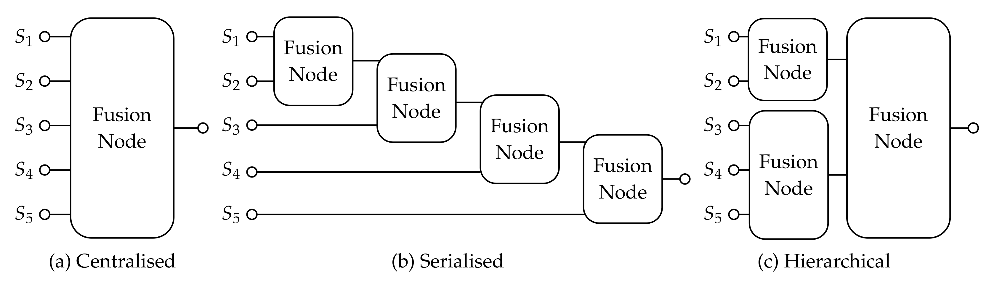
2. Fusion Topology Design in Related Work

Information fusion systems are composed of various interacting parts and methodologies, such as information sources, information pre-processing, fusion nodes, mathematical frameworks, or fusion algorithms. This results in in high-dimensional design spaces, i.e., a large amount of hyperparameters. Deciding on and designing the topology is an important subtask in fusion system design as identified by Raz et al. [16]. The authors explored the design space of a relatively simple fusion task (still $>2\times {10}^5$ design combinations) with the help of machine-learning algorithms. Their goal was to estimate the impact of design choices on the performance of the fusion system. Among other design parameters, the topology and allocation of sources to fusion nodes were identified to be crucial to the performance. This motivated ongoing work on topology design.

A widely used approach towards designing topologies and allocating information sources is to rely on meta-knowledge about the information sources. Mönks et al. [18,25] grouped information sources (here: technical sensors) into a two-level fusion topology based on the sensor’s observed objects, measured physical property, or spatial location. Semantically close (e.g., observing the same object) or spatially close sensors are assumed to be at least partly-redundant and are allocated to the same fusion node. This manual approach has been partly automated by Fritze et al. [19,26,27] who equipped sensors with a self-description containing information about the sensor’s characteristics, its contextual environment, and observed objects. A rule-based system then matches and groups sensors based on their self-description. Other ontology-based approaches have been proposed by Boury-Brisset [28] and Martí et al. [29]. Both do not focus on topology design specifically but rather on designing or facilitating a fusion system. Boury-Brisset [28] discussed ontological methods for the integration in the Joint Directors of Laboratories (JDL) fusion architecture [30] including the semantic integration of information. Martí et al. [29] proposed an ontology-based adaptive sensor fusion architecture, and this architecture organises sensors and external sources into preprocessing nodes and fusion nodes depending on the task at hand. A recent application of ontology-based design of information fusion systems can be found in the field of assisted living [31]. Ontological approaches reduce the manual effort needed for structuring fusion topologies; however, they still require profound expert knowledge about the information sources and their context. Building the ontology requires manual engineering and is time-consuming [28].

Designing information fusion topologies is closely related to the data association step predominately but not exclusively used in the JDL fusion architecture. Solaiman and Bossé [32] refer to the task of data association as the identification of any relation between information elements and monitored objects. Waltz and Llinas [33] defined the data association problem with regard to fusion systems more specifically as the “Cross correlation of measurements and m-ary decisions to partition all measurements into sets of common origin. One can distinguish between associating a set of measurements (partitioning) and associating a measurement (or a set of measurements) to a given object. […]”.

In this definition, the partitioning of measurements refers to preparing a fusion task in which each partition represents the input to a fusion node; hence, the relation to designing fusion topologies. Data-driven approaches for data association are given by Grabisch and Prade [34] and Ayoun and Smets [35]. Both approaches cluster sensor measurements based on quantifications of the measurements’ proximities. Grabisch and Prade [34] modelled information within the possibility theory and computed the proximity based on the degree of intersection of possibility distributions. Ayoun and Smets [35] used Dempster–Shafer theory instead and clustered based on the degree of conflict between measurements. A similar approach was taken by Schubert [36,37]—although not explicitly labelled as data association—who clustered basic belief functions (evidential masses) based on their conflict and attraction with each other. All of these works ([34,35,36,37]) partition information sources based on single instances of measurements (the current measurement) and not on historical data. More sophisticated interdependencies and interrelations between information sources can only be detected robustly in historical data. For example, for the identification and quantification of redundancies between sources, meaningful data are necessary, which spans over the sources’ frame of discernment as shown by Holst and Lohweg [38,39].

Regarding the problem of data association, it has to be mentioned that more recent publications focus solely on the specific application task of visual target tracking (see for example the works of Kamal et al. and Yoon et al. [40,41]). This focus comes with a shift in interpretation of the data association problem as shown by the definition given by Khaleghi et al. [42]: “[…] the data association problem, which may come in two forms: measurement-to-track and track-to-track association. The former refers to the problem of identifying from which target, if any, each measurement is originated, while the latter deals with distinguishing and combining tracks, […]”. Publications with this shifted focus are less related to the problem of designing fusion topologies.

In summary, in related works, the task of structuring fusion topologies has been approached based on expert knowledge, ontologies, or based on current measurements. Approaches that consequently analyse historical data or information in order to derive a fusion topology are missing. While this section considered topology design independently from the mathematical fusion framework, the remainder of this paper focuses on possibility theory.

3. Fusion within Possibility Theory

To provide a basis for a discussion on fusion topology design, the importance of associativity, and the role of consistency and redundancy, the core principles of possibility theory (PosT) are recapitulated. For this, common fusion rules are also reported in detail.

The main motivation behind PosT is that probability theory (ProbT) is not able to model epistemic uncertainty adequately—such as imprecision or missing information. Probability theory models random phenomena quantitatively; PosT handles incomplete information qualitatively [5,43]. Zadeh [44] introduced PosT based on fuzzy sets in the context of natural language processing. He interpreted fuzzy membership functions as possibility distributions allowing uncertainties in the sense of imprecisions as well as a lack of confidence in statements [45].

Consequently, PosT is mathematically close to fuzzy set theory [46]. This proximity often allows mathematical operations defined in the context of fuzzy sets—such as similarity measures or t-norms—to be applied to possibility distributions. Since Zadeh’s introduction of PosT, Dubois and Prade [4,6,47,48,49] and Yager [50,51,52,53] have mainly contributed to the advancement of possibility theory. If not explicitly mentioned otherwise, a numerical, real-valued representation of possibility values is assumed (cf. Dubois et al. [6] for an overview of qualitative and numerical possibility scales).

A possibility distribution is defined as a mapping of mutually exclusive and exhaustive alternative events to a numerical representation. Let the set of all alternative events be described as the frame of discernment X and let $v\in X$ be an imprecisely known element whose true value is unknown. Then, a possibility distribution is defined by

$${\pi }_v:X\to [0,1].$$

(1)

Alternatives $x\in X$ that are assigned higher values are deemed more plausible. Alternatives with ${\pi }_v\left(x\right)=0$ are considered impossible, and alternatives with ${\pi }_v\left(x\right)=1$ are fully plausible. Possibility theory is strongly guided by the minimum specificity principle, which states that any alternative x not known to be impossible should not be disregarded [45]. Extreme cases of knowledge about v are total ignorance and complete knowledge. In the first case, $\forall x\in X:{\pi }_{v}x=1$. In the case of complete knowledge, only one alternative is fully possible, and all others are impossible. A possibility distribution ${\pi }_v\left(x\right)$ is said to be normal if $\exists x\in X:{\pi }_v\left(x\right)=1$. The subset $A\subseteq X$, which $\forall x\in A:{\pi }_v\left(x\right)=1$ is referred to as core of ${\pi }_v\left(x\right)$; if $\forall x\in A:{\pi }_v\left(x\right)\ge 1$, then A is referred to as support. In the following, the shortened notation $\pi x={\pi }_{v}x$ is used.

Let multiple information sources $\mathbf{S}=\{S_1,\dots ,S_n\}$ each provide an information item $I_i$, $i\in \{1,\dots ,n\}$ in the form of a possibility distribution ${\pi }_i$ regarding the same imprecisely known element $v\in X$. A possibilistic fusion operator is then defined by $\mathit{fu}:{[0,1]}^n\to [0,1]$ and the fused possibility distribution is obtained as ${\pi }^{\left(\mathrm{fu}\right)}x=\mathit{fu}{\pi }_1\left(x\right),\dots ,{\pi }_n\left(x\right))$. Multiple information sources allow the identification of even more impossible or hardly possible alternatives for the unknown v resulting in more precise, more specific, and thus more qualitative information. In this sense, the goal in possibilistic fusion is to reach a maximal specific outcome (the most certain outcome possible) although possibility theory follows the minimum specificity principle. It is important that none of the available information is disregarded or neglected—that is, that any information source is considered by the fusion process (see also the fairness property postulated for fusion operators [6]). This fairness constraint represents the minimum specificity principle stating that alternatives that are not known to be impossible are not to be ruled out [45].

Over time, multiple possibilistic fusion operators haven been proposed, verified, and brought to applications. We propose to categorise these operators as follows:

• Possibilistic Pooling Fusion has mainly been advanced by Dubois et al. [4,48]. The aim of possibilistic pooling is to find the possibility degree for each alternative x. Hence, operators work on the grades of possibilities (by applying fuzzy norms). Inside this framework, the choice of fusion rules is most often based on the state of knowledge about the reliability of the information sources involved. Depending on reliability and available knowledge, fusion operators are distinguished into conjunctive, disjunctive, and trade-off modes [32].
• Possibilistic Estimation Fusion was mainly devised and advanced by Yager [54]. In contrast to pooling, estimation operators are based on Zadeh’s extension principle [55], which defines the use of mappings to fuzzy inputs. The goal of estimation concerns itself with finding the result that is the most compatible with all information items. Operators apply averaging functions on the frame of discernment X.
• Majority-guided Fusion identifies majority subsets—often based on consistency measures—and aggregates information from these subsets either exclusively or prioritised—similar to a voting procedure. Majority-guided fusion deliberately violates the fairness principle. It finds application in situations in which it is explicitly known that sources produce consistent readings, e.g., in redundantly engineered technical sensor systems [23]. The operators for majority-guided fusion are often based upon either pooling or fuzzy estimation as is shown in detail in the following.

3.1. Possibilistic Pooling Fusion

Conjunctive and disjunctive fusion is most commonly performed using triangular norms (t-norms) and their counterpart triangular conorms (s-norms)—both stemming from fuzzy set theory. Triangular norms and conorms are functions $\mathrm{t},\mathrm{s}:[0,1]\times [0,1]\to [0,1]$, which satisfy the properties of commutativity, associativity, and monotonicity [56]. For t-norms, 1 is the identity element, i.e., $t\pi ,1=\pi$. For s-norms, 0 is the identity element, i.e., $s\pi ,0=\pi$. Examples of t-norms are the minimum and the product operator. An example of an s-norm is the maximum operator. Although t-norms and s-norms are defined as binary functions, they can be directly applied to multiple possibility distributions because of their commutative and associative property.

In conjunctive mode, it is presumed that sources agree at least partially about the possibility of alternatives, that is, their information items are at least partially consistent. Consistency within a group of information items $\mathbf{I}$ is defined as [4]

$$h(\mathbf{I})=h({\pi }_1,{\pi }_2,\dots ,{\pi }_n)=\underset{x\in X}{max}\left(\underset{i\in \{1,\dots ,n\}}{t}({\pi }_i(x))\right).$$

(2)

Partially agreeing sources are characterised by items with $h(\mathbf{I})>0$—that is, their possibility distributions have overlapping support. Fully agreeing sources have items with $h(\mathbf{I})=1$, i.e., their possibility distributions have overlapping cores. Conjunctive fusion of fully consistent information items is then achieved by directly applying a t-norm [48]:

$${\pi }^{\left(\mathrm{fu}\right)}(x)=\underset{i\in \{1,\dots ,n\}}{t}({\pi }_i\left(x\right)).$$

(3)

As t-norms satisfy the strong zero preservation principle, i.e., $t(\pi ,0)=0$, the conjunctive fusion excludes all alternatives, which at least one information source deems impossible. Conjunctive fusion results in the most specific outcome by eliminating alternatives. If information items are only partially consistent, then fusion based on t-norms results in subnormal possibility distributions. Renormalising the resulting possibility distribution leads to

$${\pi }^{\left(\mathrm{fu}\right)}x=\frac{{\displaystyle \underset{i\in \{1,\dots ,n\}}{t}({\pi }_i\left(x\right))}}{{\displaystyle \underset{i\in \{1,\dots ,n\}}{h}({\pi }_i)}},$$

(4)

which is only defined if sources are not completely disagreeing and if their information items not fully inconsistent, i.e., $h\ne 0$ [48].

The disjunctive fusion is appropriate if information items are completely inconsistent, i.e., sources disagree, at least one of them is wrong in its assessment, and it is not known which one. The disjunctive fusion is given by applying an s-norm:

$${\displaystyle {\pi }^{\left(\mathrm{fu}\right)}(x)=\underset{i\in \{1,\dots ,n\}}{s}({\pi }_i\left(x\right))}$$

(5)

keeping all available information. In general, purely disjunctive fusion is not desirable as it results in minimal specific outcomes but is necessary in disagreeing cases.

Trade-off fusion modes combine conjunctive and disjunctive fusion depending on what is known (or assumed) about the reliability of sources. Prominent fusion rules can be found in the paper of Dubois and Prade [4]. For this paper, the most important of these are fusion based on the most consistent subsets, quantified fusion, and adaptive fusion.

One prominent way to aggregate information in a two-step process is to search for maximal consistent subsets (MCS) [20,57]. These nonconflicting MCS are fused conjunctively prior to disjunctive fusion of intermediate results. Dubois et al. [58] proposed an algorithm that finds MCS with linear complexity. In this algorithm, all subsets of $\mathbf{I}$ with a consistency above or equal to $\alpha \in [0,1]$ are clustered. Let ${\mathbf{I}}^{\mathrm{MCS}}\subseteq \mathbf{I}$ denote MCS subsets, then MCS fusion is formalised for a possibilistic setting as [6]:

$${\pi }^{\left(\mathrm{fu}\right)}(x)=\underset{{\mathbf{I}}^{\mathrm{MCS}}\subseteq \mathbf{I}}{max}\left(\underset{I_i\in {\mathbf{I}}^{\mathrm{MCS}}}{t}({\pi }_i\left(x\right))\right).$$

(6)

Later advancements in MCS fusion were proposed in multiple works [59,60,61].

Quantified fusion [62,63] is a similar two-step fusion process, which assumes that the number of reliable sources j is known. The quantified rule then takes all subsets of information items ${\mathbf{I}}_{*}\subseteq \mathbf{I}$ with cardinality j and fuses these conjunctively in the first step. All intermediate results are then fused disjunctively:

$${\pi }^{\left(\mathrm{fu}\right)}(x)=\underset{\begin{array}{c}{\mathbf{I}}_{*}\subseteq \mathbf{I}\\ |{\mathbf{I}}_{*}|=j\end{array}}{max}\left(\underset{I_i\in {\mathbf{I}}_{*}}{min}({\pi }_i\left(x\right))\right).$$

(7)

Adaptive fusion aims at progressing gradually from conjunctive to disjunctive behaviour as conflict increases. A simple adaptive fusion rule is

$${\pi }^{\left(\mathrm{fu}\right)}(x)=max\left(\frac{{\displaystyle \underset{i\in \{1,\dots ,n\}}{min}({\pi }_i(x))}}{{\displaystyle \underset{i\in \{1,\dots ,n\}}{h}({\pi }_i)}},min\left(\underset{i\in \{1,\dots ,n\}}{max}({\pi }_i(x)),1-\underset{i\in \{1,\dots ,n\}}{h}({\pi }_i)\right)\right).$$

(8)

It fuses all sources disjunctively (assuming one source is right) and discounts the result by $(1-h)$. In parallel, it fuses all sources conjunctively (assuming all sources are right) and combines both intermediate results. This process does not consider situations in which more than one or less than all sources are reliable. If many sources are fused, it is likely that $h\to 0$, thus, resulting in uninformative results [4]. Dubois’ adaptive fusion rule [4,48] builds upon the quantified (7) and adaptive fusion rule (8) assuming that a minimum and maximum number of reliable sources are known. The minimum and maximum number are derived from the consistency of information items $\mathbf{I}$. The cardinality of the largest fully consistent subset gives the minimum number $j^{-}=max(\left|\mathbf{I}\right||h(\mathbf{I})=1)$; the largest partially consistent subset provides the maximum number $j^{+}=max(\left|\mathbf{I}\right||h(\mathbf{I})>0)$. The adaptive fusion is then

$${\pi }^{\left(\mathrm{fu}\right)}(x)=max\left(\frac{{\displaystyle {\pi }_{+}^{\left(fu\right)}(x)}}{{\displaystyle \underset{i\in \{1,\dots ,n\}}{h}({\pi }_i)}},min\left({\pi }_{-}^{\left(fu\right)}(x),1-h_{+}\right)\right)$$

(9)

in which ${\pi }_{+}^{\left(fu\right)}(x)$ and ${\pi }_{-}^{\left(fu\right)}(x)$ are obtained by quantified fusion (7) (with $j^{-}$ and $j^{+}$, respectively) and $h_{+}={max}_{I_{*}\subseteq \mathbf{I}\left|\right|I_{*}|=j^{+}}(h(I_{*}))$. In this way, completely disagreeing sources with fully inconsistent items ($h=0$) are disregarded. Furthermore, small changes in the input possibility distributions may lead to significant changes in the fusion result [64].

Oussalah et al. [64] proposed changes to (9) improving the behaviour in the case of outliers and with regard to robustness against small changes. For their progressive fusion rule, they introduced a distance measurement with which the disjunctive fusion (${\pi }_{-}^{\left(fu\right)}(x)$) part is adapted. Let $x_0,x_1\in X$ be the smallest and largest element of the consensus set, then

$$d(x)=\left\{\begin{array}{cc}max(|x-x_0|,|x-x_1|)\hfill & \mathrm{if}x<x_0\mathrm{or}x>x_1,\hfill \\ 0\hfill & \mathrm{otherwise},\hfill \end{array}\right.$$

measures the distance from point x to the consensus set. Let $\alpha (x)=min\left(\frac{d(x)}{d_0},1\right)$ be a weighting factor. The threshold $d_0$ is the maximum distance until outliers are considered. Then, ${\pi }_{-}^{\left(fu\right)}(x)$ in (9) is replaced by

$${\pi }_{-}^{\left(fu\right)}(x)=\alpha (x)·{\pi }_{+}^{\left(fu\right)}(x)+(1-\alpha (x))·\underset{i\in \{1,\dots ,n\}}{max}({\pi }_i\left(x\right)).$$

(10)

Instead of (9), (10) considers the completely disjunctive fusion of all information items. The degree to which it considers disjunction relies on $d(x)$. The further x is from the consensus set, the more consideration is given to inconsistent items.

3.2. Possibilistic Estimation Fusion

Whereas pooling fusion aims at discarding alternatives, estimation fusion assumes that none of the sources are completely wrong and attempts to find a fusion result that is compatible with all information items [4]. Nonetheless, more specific or precise outcomes are still preferable. Estimation fusion has received less attention in the scientific community compared with pooling fusion (The higher number of citations of Dubois’s paper [4] compared to Yager’s paper [65] reflect the higher attention). Therefore, the following discussion takes a deeper look into the algebraic properties of estimation fusion.

Estimation fusion is based on Zadeh’s extension principle, which allows mapping functions to be used on fuzzy sets [66]. Let $Y,Z$ be a frame of discernments and $F:Y\to Z$. Let A be a fuzzy set defined on Y and B a fuzzy set defined on Z, and then F maps the fuzzy membership function ${\mu }_A(y)$ with $y\in Y$ to ${\mu }_B(z)$ with $z\in Z$ by ${\mu }_B(z)={\mu }_A\left(F^{-1}(z)\right)={\mu }_A(y)$ with $z=F(y)$. If F results in multiple outputs for the same y, then

$${\mu }_B(z)=\underset{y\in Y:F\left(y\right)=z}{max}{\mu }_A(y).$$

In multi-source estimation fusion, the input possibility distributions are first pooled by a fusion function—here referred to in this context as G. The result is then mapped by the multi-parameter function $F(x_1,x_2,\dots ,x_n)$ with $x_i\in X_i$, $i\in \{1,\dots ,n\}$ onto a new frame of discernment X, i.e.,

$${\pi }^{\left(\mathrm{fu}\right)}(x)=\underset{\begin{array}{c}{x}_i\in X_i:F(x_1,\dots ,x_n)=x\end{array}}{max}\left(\underset{i}{G}({\pi }_i\left(x_i\right))\right),$$

(11)

for which the notation

$${\pi }^{\left(\mathrm{fu}\right)}(x)=\left\{\frac{G({\pi }_1\left(x_1\right),{\pi }_2\left(x_2\right),\dots ,{\pi }_n\left(x_n\right))}{F(x_1,x_2,\dots ,x_n)}\right\}.$$

(12)

is used in the following. The fusion rule in (11) takes the maximum of $G_i({\pi }_i\left(x_i\right))$ for every n-tuple $(x_1\in X_1,\dots ,x_n\in X_n)$, which satisfies $F(x_1,\dots ,x_n)=x$.

Yager [65] proposed an estimation fusion rule in which G is the minimum operator and F is defined to be an averaging operator.

Definition 3

(Averaging Operator). An operator that satisfies the three properties of commutativity, monotonicity, and idempotency, is referred to as a mean or averaging operator [4]. Such an averaging operator $avg\left(·\right)$ lies between $min\left(·\right)$ and $max\left(·\right)$, i.e., $min\left(·\right)\le avg\left(·\right)\le max\left(·\right)$.

Yager’s estimation fusion rule [65] is then:

$${\pi }^{\left(\mathrm{fu}\right)}(x)=\left\{\frac{{\displaystyle \underset{i\in \{1,\dots ,n\}}{min}({\pi }_i\left(x_i\right))}}{F(x_1,x_2,\dots ,x_n)}\right\}.$$

(13)

The application of the minimum operator results in maximal specific possibility distributions, which are placed on an averaged frame of discernment. The disadvantages of estimation fusion are that (i) it requires a frame of discernment for which it is sensible to apply averaging operators on and that (ii) estimation fusion may lead to fusion results that have been deemed impossible by all sources, i.e., the results do not satisfy the zero preservation principle [4]. Regarding the first disadvantage, it is often assumed that $X\subseteq \mathbb{R}$ [65], which is also assumed for the remainder of this section.

If G is also an averaging operator, then a noteworthy interaction between estimation fusion and the frame of discernment takes place, which is relevant for practical implementations.

Proposition 1.

If G is an averaging operator other than the minimum operator and $X\subseteq \mathbb{R}$, then fusion with (13) is influenced by the borders of X. More formally, ${min}_{{\pi }^{\left(\mathrm{fu}\right)}(x)>0}x$ is dependent on ${min}_{x\in X}x$ and ${max}_{{\pi }^{\left(\mathrm{fu}\right)}(x)>0}x$ on ${max}_{x\in X}x$.

Proof. 

Let ${\displaystyle x_{\mathrm{a}}=\underset{x\in X}{min}x}$ and ${\displaystyle x_{\mathrm{b}}=\underset{x\in X}{max}x}$, i.e., $X=[x_{\mathrm{a}},x_{\mathrm{b}}]$. Let ${\displaystyle x^{\prime }=\underset{i}{min}\underset{x_i\in X_i:{\pi }_i(x_i)>0}{min}{x}_i}$, i.e., $x^{\prime }$ is the smallest element in X for which at least one ${\pi }_i>0$. Furthermore, let ${\displaystyle i^{\prime }=\underset{i}{arg\; min}\underset{x_i\in X_i:{\pi }_i{x}_i>0}{min}(x_i)}$. If $G\ne min$, then, for at least one permutation of the n-tuple $(x_{\mathrm{a}},x_{\mathrm{a}},\dots ,x^{\prime },\dots ,x_{\mathrm{a}},x_{\mathrm{a}})$: $G\left({\pi }_1\left(x_{\mathrm{a}}\right),\dots ,{\displaystyle \underset{\underset{>0}{︸}}{{\pi }_{i^{\prime }}\left(x^{\prime }\right)}},\dots ,{\pi }_n\left(x_{\mathrm{a}}\right)\right)>0$. This n-tuple defines the minimum boundary of ${\pi }^{\left(\mathrm{fu}\right)}$, i.e., ${\displaystyle \underset{{\pi }^{\left(\mathrm{fu}\right)}(x)>0}{min}x=F(x_{\mathrm{a}},\dots ,x^{\prime },\dots ,x_{\mathrm{a}})}$. The same holds for the maximum boundary of ${\pi }^{\left(\mathrm{fu}\right)}$ only that ${\displaystyle x^{\prime }=\underset{i}{max}\underset{x_i\in X_i:{\pi }_i(x_i)>0}{max}{x}_i}$, ${\displaystyle i^{\prime }=\underset{i}{arg\; max}\underset{x_i\in X_i:{\pi }_i(x_i)>0}{max}{x}_i}$, and ${\displaystyle \underset{{\pi }^{\left(\mathrm{fu}\right)}(x)>0}{max}x=F(x_{\mathrm{b}},\dots ,x^{\prime },\dots ,x_{\mathrm{b}})}$.    □

An example of the effects of Proposition 1 is illustrated in Figure 2.

Corollary 1.

If X is also unbounded and F is an averaging operator other than the minimum or maximum operator, then (13) results in an unbounded ${\pi }^{\left(\mathrm{fu}\right)}$. If X is half-bounded, then ${\pi }^{\left(\mathrm{fu}\right)}$ is also half-bounded.

Proof. 

From Proposition 1 it follows directly that, if $F\ne max$, then ${\displaystyle \underset{x_{\mathrm{a}}\to -\infty }{lim}\underset{{\pi }^{\left(\mathrm{fu}\right)}(x)>0}{min}x}$$=F(x_{\mathrm{a}},\dots ,x^{\prime },\dots ,x_{\mathrm{a}})=-\infty$. If $F\ne min$, then ${\displaystyle \underset{x_{\mathrm{b}}\to \infty }{lim}\underset{{\pi }^{\left(\mathrm{fu}\right)}(x)>0}{max}x=F(x_{\mathrm{b}},\dots ,x^{\prime },\dots ,x_{\mathrm{b}})}$$=\infty$.    □

Consequently, if G is an averaging operator other than the minimum operator, then it is reasonable to apply estimation fusion only on bounded X. Otherwise, (12) and (13) lead to fusion results spanning to infinity—even for very precise input possibility distributions.

3.3. Majority-Guided Fusion

In essence, fusion rules, which focus and prioritise the consensus set—often also referred to as majority observation—fall under the category of majority-guided fusion. Majority-guided fusion is particularly sensible in cases in which information sources are known to produce consistent items. Possibility distributions deviating from the consensus set are then deduced to be faulty (unreliable) instead of giving useful information about the unknown value v.

With this in mind, Dubois’ fusion rule (9) already satisfies as a majority-guided fusion rule because it ignores all inconsistent information items (although this fact is precisely one of the main points of criticism by Oussalah et al. [64]). In the specific case of assuming fully reliable sources and expecting consistency between items, it is reasonable to rely on simpler fusion rules; accordingly, it was proposed to use a purely conjunctive fusion rule [23]. Similarly simple are counting fusion functions; the result here is the alternative that most sources consider possible [5].

Estimation fusion rules, such as (13), favour the majority observation because of the averaging characteristic of the estimation operator F. A more complex majority-guided fusion rule, which is based on Yager’s estimation fusion (13), was proposed by Glock et al. [67], the majority-opinion-guided possibilistic fusion rule (MOGPFR). The MOGPFR replaces both the conjunctive fusion part G and the estimation operator F with the Implicative Importance Weighted Ordered Weighted Averaging (IIWOWA) operator. The IIWOWA operator, as proposed by [68], is an extension of the parent class of Ordered Weighted Averaging (OWA) operators [50]. An OWA operator allows weighting inputs with $\mathbf{w}=(w_1,\dots ,w_n)$, $w_i\in [0,1]$, and ${\sum }_i{w}_i=1$. Inputs ${\pi }_i$ are ordered in descending order. This results in aggregation $\frac{1}{n}\sum w_i·{\pi }_i$ and allows the aggregation to be shifted between the minimum with $\mathbf{w}=(0,0,\dots ,1)$ and maximum $\mathbf{w}=(1,\dots 0,0)$. The MOGPFR is then defined as follows:

$$\begin{array}{c}{\pi }^{\left(\mathrm{fu}\right)}(x)={\displaystyle \underset{i}{max}}({\mathit{rel}}_i)·{\widehat{\pi }}^{\left(fu\right)}(x)+1-{\displaystyle \underset{i}{max}}({\mathit{rel}}_i),\mathrm{with}\\ {\widehat{\pi }}^{\left(fu\right)}(x)=\left\{\frac{{\displaystyle \underset{i\in 1,\dots ,n}{{\lambda }_{\mathrm{IIWOWA}}}\left(\mathbf{v},{\mathbf{w}}_{\mathrm{p}},{\pi }_i({\mu }^{\left(i\right)})\right)}}{{\displaystyle \underset{i\in 1,\dots ,n}{{\lambda }_{\mathrm{IIWOWA}}}\left(\mathbf{v},{\mathbf{w}}_{\mathrm{m}},{\mu }^{\left(i\right)}\right)}}\right\};\end{array}$$

(14)

in which ${\lambda }_{\mathrm{IIWOWA}}(\circ )$ denotes the IIWOWA operator, and ${\mathit{rel}}_i$ is the reliability for each source. The MOGPFR specifically allows the control of fusion by (i) a reliability vector $\mathbf{v}=\{v_1,v_2,\dots ,v_n\}$ with $v_i\in [0,1]$, which discounts informations items and (ii) two weighting vectors, ${\mathbf{w}}_p$ and ${\mathbf{w}}_m$, which control whether G and F are close to the minimum or maximum operator, respectively. The IIWOWA operator is defined only for inputs in $[0,1]$, which necessitates the fuzzification of X so that the possibility distributions become ${\pi }_i\left({\mu }^{\left(i\right)}\right)$.

The MOGPFR facilitates the prioritisation of information items belonging the majority observation. The importance values $v_i$ are determined by a distance function of ${\pi }_i$ to the majority set; the possibility distribution ${\pi }_i$ is discounted accordingly. The parameters ${\mathbf{w}}_p$ and ${\mathbf{w}}_m$ allow adapting fusion towards conjunctive and disjunctive behaviour. The benefit gained by the MOGPFR lies in its level of control through parametrisation.

4. Approach towards Topology Design

Associative fusion rules allow changing the sequence in which information sources are fused without altering the fusion result. Therefore, associativity is a beneficial property with regard to the topology design of distributed information fusion systems. Assuming associativity, a system designer or a design algorithm can focus on other criteria for designing a fusion system, such as spatial availability of sources or consistency as well as the redundancy of sources. In this section, we analyse the presented fusion rules regarding the associativity property and its impact on topology design. Following this, a two-layer fusion topology based on the MCS fusion rule (6) is presented. Consistency as a design criterion both increases the specificity of fusion results due to the minimum-operator [6] and to facilitate source defect detection algorithms [21,22]. This motivates the dive into the MCS fusion topologies in this article.

Some flaws and shortcomings of this consistency-based approach are discussed, which leads to several adjustments to overcome those. This includes the introduction of redundancy as a design criterion.

First, both fusion node and fusion topology are defined, and some notations introduced:

Definition 4

(Fusion Node). A fusion node $\mathit{fn}$ is a self-contained module encapsulating a fusion operator. A node takes information items as input and outputs a single fused information item. As a node is a self-contained module, a fusion node and its fusion operator have to satisfy the following additional properties:

• Modularity: A fusion node outputs a fused information item, which qualifies as a possibility distribution π (see Section 3), i.e., π is normal. This property allows self-contained intermediate results in a topology and makes fusion nodes modular. This increases the transparency of the distributed fusion topology.
• Self-Reproducing: Given a single input, a fusion node reproduces this input. It preserves its identity, i.e., $\mathit{fu}(I)=I$.

Idempotency as a property is not required since idempotency restricts the fusion node in the case where a reinforcement effect is desired (e.g., via the product operator as a t-norm). A fusion node with an associative fusion operator is beneficial since it allows splitting the fusion node.

A fusion node is a modular part of a fusion topology. In order to facilitate the fusion process of the grander topology, it may output auxiliaries denoted as $\left[\mathit{AUX}\right]$. Consequently, a node is also required to be able to process $\left[\mathit{AUX}\right]$ as input if necessary.

Definition 5

(Fusion Topology). Interconnected fusion nodes build up a fusion topology. Fusion nodes may be interconnected parallelly, serially, hierarchically, cascadingly, or in more complex structures. A fusion topology organises a feed forward flow of information. Recursive interconnections are excluded. A fusion topology is constructed in layers $l\in {\mathbb{N}}_{>0}$. In each layer, fusion nodes are indexed consecutively with $k\in {\mathbb{N}}_{>0}$. The k-th fusion node in layer l is denoted by ${\mathit{fn}}_{(k,l)}$, its output information item by $I_{(k,l)}$, and its auxiliary output by ${\left[\mathit{AUX}\right]}_{(k,l)}$.

Given the above definitions, Figure 3 shows a three-layer example topology to help visualise the introduced notations.

The MCS-based design presented in this article focuses on a two-layer topology by grouping consistent or redundant information sources into fusion nodes. For an easier reading of the article, fusion nodes are also denoted as ${\mathit{fn}}_{\left(k\right)}$ in a two-layer topology. Since this approach considers associative fusion rules, the basic two-layer design can be easily extended into a multi-layer version.

4.1. Associativity

In possibilistic information fusion, the fusion process is rarely considered to be distributed. As a consequence, possibilistic fusion rules are often not associative, which heavily alters the fusion results in differently structured topologies. However, in works regarding possibilistic fusion, associativity has been considered with low priority at best and neglected at worst. For instance, associativity is described as a useful property by Dubois et al. [6]; however, its absence is not considered to be a fatal flaw.

As a first step in discussing associativity, the fusion rules presented in the previous section are summarised in

Table 1. Common fusion rules and the property of (quasi-)associativity.

Fusion Rule	Equation(s)	Associative	Proof of Associativity	Quasi-Associative	Proof of Quasi-Associativity
Conjunctive	(3)	yes	Inherited from t-norm	yes	See Proposition 2
Renormalised Conjunctive	(4)	Dependent on t-norm	Proof for nonassociativity in the case of minimum-norm and associativity in the case of product-norm given by Dubois and Prade [47]	yes	${\displaystyle f_{\left(k\right)}\left({\mathbf{I}}_{\left(k\right)}\right)=t\left({\mathbf{I}}_{\left(k\right)}\right(}$ and $g=\frac{1}{h(f_{\left(k\right)}{\mathbf{I}}_{\left(k\right)})}$
Disjunctive	(5)	yes	Inherited from s-norm	yes	See Proposition 2
MCS fusion	(6)	no	[61]	no	[61]
Quantified	(7)	no	Proof given in Appendix B	no	Similar to MCS fusion
Adaptive	(8), (9)	no	[69]	no	[69]
Progressive	(9), (10)	no	Inherited from adaptive fusion	no	Inherited from adaptive fusion
Estimation	(13)	yes (with restrictions)	See Proposition 3	yes (with restrictions)	See Propositions 2 and 3
MOGPFR	(14)	no	Proof given in Appendix B	no	OWA operator prevents quasi-associativity

.

The table also shows whether the rules satisfy the following two properties:

Definition 6

(Associativity). A fusion operator $\mathit{fu}$ is associative if the fusion outcome is independent of the sequence in which information items are fused, i.e., $\mathit{fu}(I_1,I_2,I_3)=\mathit{fu}(\mathit{fu}(I_1,I_2),I_3)$$=\mathit{fu}(I_1,\mathit{fu}(I_2,I_3))$.

Definition 7

(Quasi-associativity). A fusion operator $\mathit{fu}$ is quasi-associative if it can be expressed as a sequence of associative steps and a final operation acting on the results of the previous associative steps [47]. Let f be an associative function and g be a function not restricted to the associativity property, then $\mathit{fu}$ is quasi-associative if $\mathit{fu}(I_1,I_2,I_3)=g(f(f(I_1,I_2),I_3))=g(f(I_1,f(I_2,I_3)))$.

Proposition 2.

If a fusion operator is associative, then it is also quasi-associative.

Proof. 

Let $\mathbf{I}$ be a set of information items, let $f=\mathit{fu}$ and g be an identity function: $g(\mathbf{I})=\mathbf{I}$. Then, $g(f(\mathbf{I}))=\mathit{fu}(\mathbf{I})$—that is, by making use of an identity function, an associative fusion operator becomes quasi-associative.    □

From this, it follows that, if a fusion rule is not quasi-associative, then it is also not associative.

Associative rules allow unrestricted topology design in the sense that sources can be freely assigned to fusion nodes without changing the overall fusion result. Quasi-associative rules require a final centralised fusion step in which the nonassociative part is computed. The associative part can be distributed to fusion nodes.

4.1.1. Pooling Fusion

As can be seen in Table 1, the simple conjunctive and disjunctive fusion rules satisfy associativity. However, depending on the applied t-norm—the renormalisation step already causes nonassociative behaviour. For the product norm ($\mathrm{t}({\pi }_1(x),{\pi }_2(x))={\pi }_1(x)·{\pi }_2(x)$), fusion stays associative; however, generally, renormalisation prevents associativity [47].

MCS fusion (6) is based on the idea that consistent information items are to be fused conjunctively first before the results are fused disjunctively. MCS fusion thus specifies a sequence in which information is to be fused. Consequently, MCS fusion is not associative. It is quite easy to see that different sequences result in different outcomes (see Appendix B for an example). Quantified fusion (7) has a similar approach, meaning that it fuses conjunctively and disjunctively in two steps. Quantified fusion is—for the same reasons as MCS fusion—not associative and not quasi-associative.

More sophisticated fusion rules—such as adaptive (8), (9) and progressive (10) rules—attempt to make the most of all available information. These fusion rules rely on specific metrics, such as global consistency, consistency between specific subsets, or distances between information items. Many of these metrics are only computable if all information items are available centrally. Since all three rules (8), (9), and (10) are based on the quantified fusion rule, they inherit quantified fusion’s nonassociativity.

4.1.2. Estimation and Majority-Guided Fusion

Estimation fusion (11)–(13) as well as the majority-guided MOGPFR (14) relies on Zadeh’s extension principle.

Proposition 3.

With regard to Zadeh’s extension principle, a fusion operator $\mathit{fu}({\pi }_1,{\pi }_2,{\pi }_3)=\left\{\frac{G({\pi }_1\left(x_1\right),{\pi }_2\left(x_2\right),{\pi }_3\left(x_3\right))}{F(x_1,x_2,x_3)}\right\}$ satisfies associativity if G and F are associative functions and G is monotonic increasing in all its arguments.

Proof. 

The operator $\mathit{fu}$ is associative if $\mathit{fu}({\pi }_1,{\pi }_2,{\pi }_3)=\mathit{fu}({\pi }_1,\mathit{fu}({\pi }_2,{\pi }_3))$. With (11), this becomes

$$\begin{array}{c}\underset{x_i\in X_i:F(x_1,x_2,x_3)=x}{max}G({\pi }_1\left(x_1\right),{\pi }_2\left(x_2\right),{\pi }_3\left(x_3\right))=\hfill \\ \hfill \underset{\begin{array}{c}{x}_1\in X_1,x^{\prime }\in X^{\prime }:\\ F(x_1,x^{\prime })=x\end{array}}{max}G\left({\pi }_1\left(x_1\right),\underset{\begin{array}{c}{x}_2\in X_2,x_3\in X_3:\\ F(x_2,x_3)=x^{\prime }\end{array}}{max}G({\pi }_2\left(x_2\right),{\pi }_3\left(x_2\right))\right).\end{array}$$

The frame of discernment $X^{\prime }$ contains every unique element given by $F((x_2,x_3)$ for every 2-tuple $(x_2,x_3)$ with $x_2\in X_2$ and $x_3\in X_3$. In the following, the notation ${\displaystyle \underset{\begin{array}{c}{x}_2\in X_2,x_3\in X_3:\\ F(x_2,x_3)=x^{\prime }\end{array}}{max}}$ is shortened to ${\displaystyle \underset{\begin{array}{c}F(x_2,x_3)=x^{\prime }\end{array}}{max}}$—this also applies to similar notations.

Assume G to be monotonic increasing in all its arguments, i.e., for any $a_i,b_i\in [0,1]$ with $i\in \{1,2,\dots ,n\}$ and $\forall i:a_i\le b_i$: $G(a_1,a_2,\dots ,a_n)\le G(b_1,b_2,\dots ,b_n)$. If ${\pi }_1\left(x_1\right)\ge G({\pi }_2\left(x_2\right),{\pi }_3\left(x_2\right))$, then $G({\pi }_2\left(x_2\right),{\pi }_3\left(x_2\right))$ has no influence on the term $max(G({\pi }_1\left(x_1\right),G({\pi }_2\left(x_2\right),{\pi }_3\left(x_2\right))))$. If, on the other hand, ${\pi }_1\left(x_1\right)<G({\pi }_2\left(x_2\right),{\pi }_3\left(x_2\right))$, then $G({\pi }_1\left(x_1\right),G({\pi }_2\left(x_2\right),{\pi }_3\left(x_2\right)))$ becomes maximal if $G({\pi }_2\left(x_2\right),{\pi }_3\left(x_3\right))$ is maximal. Consequently,

$$\begin{array}{cc}\hfill \mathit{fu}({\pi }_1,\mathit{fu}({\pi }_2,{\pi }_3))& =\underset{\begin{array}{c}F(x_1,x^{\prime })\end{array}=x}{max}G\left({\pi }_1\left(x_1\right),\underset{\begin{array}{c}F(x_2,x_3)=x^{\prime }\end{array}}{max}G({\pi }_2\left(x_2\right),{\pi }_3\left(x_2\right))\right)\hfill \\ \hfill & =\underset{\begin{array}{c}F(x_1,x^{\prime })=x\end{array}}{max}\underset{\begin{array}{c}F(x_2,x_3)=x^{\prime }\end{array}}{max}G({\pi }_1\left(x_1\right),G({\pi }_2\left(x_2\right),{\pi }_3\left(x_2\right))).\hfill \end{array}$$

If G is also associative, then

$$\begin{array}{cc}\hfill \mathit{fu}({\pi }_1,\mathit{fu}({\pi }_2,{\pi }_3))& =\underset{\begin{array}{c}F(x_1,x^{\prime })=x\end{array}}{max}\underset{\begin{array}{c}F(x_2,x_3)=x^{\prime }\end{array}}{max}G({\pi }_1\left(x_1\right),{\pi }_2\left(x_2\right),{\pi }_3\left(x_2\right)).\hfill \end{array}$$

If F is associative, then

$$\begin{array}{cc}\hfill \mathit{fu}({\pi }_1,\mathit{fu}({\pi }_2,{\pi }_3))& =\underset{\begin{array}{c}F(x_1,x_2,x_3)=x\end{array}}{max}G({\pi }_1\left(x_1\right),{\pi }_2\left(x_2\right),{\pi }_3\left(x_2\right)).\hfill \end{array}$$

   □

In contrast to the estimation fusion rules, the MOGPFR (14) uses the IIWOWA operator for the functions F and G and is, therefore, not associative. The IIWOWA operator is an extension of the OWA operator. The OWA operator sorts the inputs $({\pi }_1(x_1),\dots ,{\pi }_n(x_n))$ in descending order. It then weights the inputs with a predefined weighting vector $(w_1,\dots w_n)$ with $w_i\in [0,1]$. For $(1,0,\dots ,0)$ the OWA operator becomes the maximum operator, and for $(0,\dots ,0,1)$, the minimum operator. In these cases, the OWA operator is associative. In all other cases, sorting the input values prevents associativity and quasi-associativity. Consequently, the IIWOWA operator and the MOGPFR are nonassociative as well.

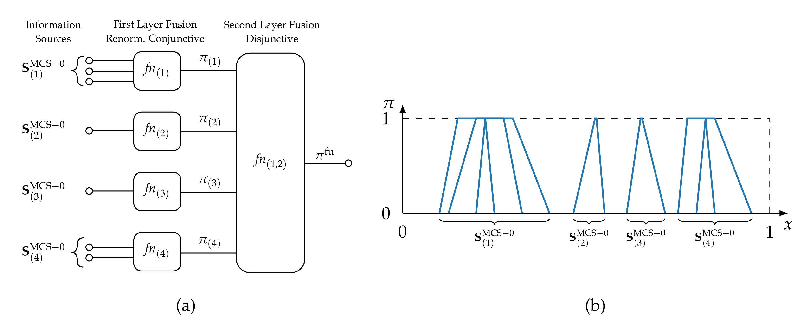
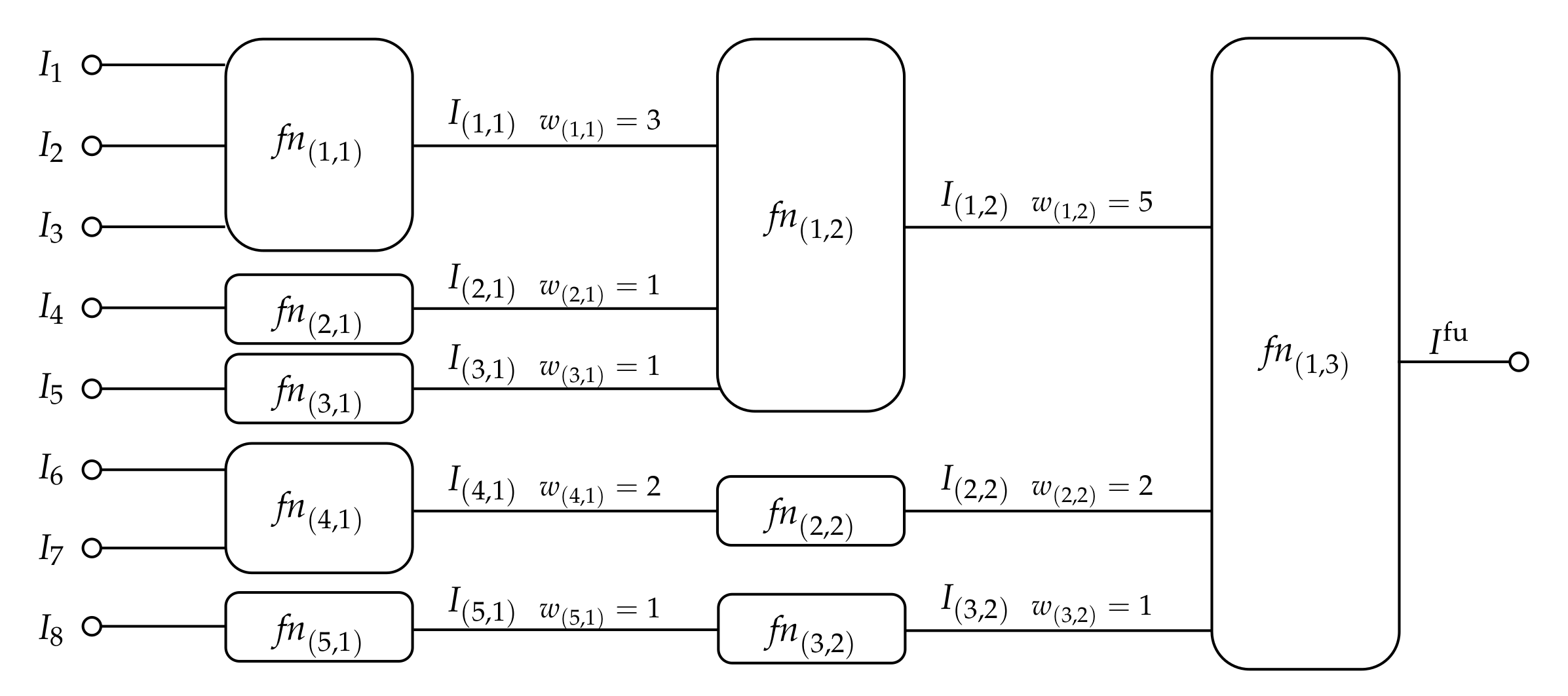
4.2. MCS-Based Topology Design

In addition to relying on associative and quasi-associative rules, there is the third option to design a fusion topology and its fusion process based on the characteristics of the information items themselves. In this case, the possibility distributions of sources are analysed, which guides the design towards desired effects. In a sense, the information provided by the multi-source system dictates the topology.

One approach to do so is to build upon the MCS fusion rule (6). It itself is not quasi-associative, and thus information items cannot be freely assigned to fusion nodes. However, by carefully searching for all the most consistent subsets, fusion can be distributed in a way that each fusion node produces the most specific intermediate result from agreeing sources, thus, emphasizing the consensus of this agreeing subset. In such a two-layer topology, all $I\in {\mathbf{I}}_{\left(k\right)}^{\mathit{MCS}-\alpha }$ are fused in separate fusion nodes ${\mathit{fn}}_{\left(k\right)}$ using, at the first level, a mix of renormalised conjunctive minimum fusion and maximum fusion:

$${\pi }_{\left(k\right)}(\mu )=\left\{\begin{array}{cc}\frac{{min}_i{\pi }_i(\mu )}{h_i({\pi }_i(\mu ))}\hfill & \mathrm{if}{h}_i({\pi }_i(\mu ))>0\hfill \\ \underset{i}{max}{\pi }_i(\mu )\hfill & \mathrm{if}{h}_i({\pi }_i(\mu ))=0\hfill \end{array}\right.$$

(15)

with i indexing $I_i\in {\mathbf{I}}_{\left(k\right)}^{\mathrm{MCS}-\alpha }$. At the second level, all intermediate results are fused disjunctively using the maximum operator. An exemplary fusion topology based on the MCS fusion rule is shown in Figure 4.

As MCS fusion analyses the consistency of information items, the inferred topology needs to be adapted for each new set of items. This is, particularly in a technical system, often not practical or feasible. Think, for example, of a technical multi-sensor system in which sensors give updated measurements in periodic time increments. In this case, the advantages of distributed fusion—such as the distribution of computing load into local nodes or lower communication loads by condensing information—are negated by the reorganisation with each measurement. Finding the MCS requires having all information items at hand in one central node rendering the distribution of the fusion process pointless. Therefore, topology design based on MCS fusion is only beneficial, if knowledge about the sources’ expected behaviour regarding consistency exists a priori. In other words, if it is known that sources produce consistent items continually, then they are assigned to a fusion node without the need for an update with each new instance or measurement. This knowledge can be derived or learned from representative training data. Conclusions about the sources’ consistency in the training data are used to build up the MCS fusion topology.

Let ${\mathbf{S}}_{\left(k\right)}^{\mathrm{MCS}-\alpha }$ be a set of information sources that are assigned to fusion node ${\mathit{fn}}_{\left(k\right)}$. Furthermore, let $j=\{1,\dots ,m\}$ be indices of training data, $I_{\left(k\right),j}$ be an information item produced by source $S_{\left(k\right)}$ at instance j, and ${\mathbf{I}}_{\left(k\right),j}$ be all information items of ${\mathbf{S}}_{\left(k\right)}^{\mathrm{MCS}-\alpha }$ at instance j, then

$$S_{\left(k\right)}\in {\mathbf{S}}_{\left(k\right)}^{\mathrm{MCS}-\alpha }\mathrm{if}\left\{\begin{array}{cc}\forall j=\{1,\dots ,m\}:h\left(I_{\left(k\right),j},{\mathbf{I}}_{\left(k\right),j}\right)\ge \alpha \hfill & \mathrm{and}\mathrm{if}\alpha \in (0,1],\hfill \\ \forall j=\{1,\dots ,m\}:h\left(I_{\left(k\right),j},{\mathbf{I}}_{\left(k\right),j}\right)>0\hfill & \mathrm{and}\mathrm{if}\alpha =0,\hfill \end{array}\right.$$

(16)

i.e., a source $S_{\left(k\right)}$ belongs to ${\mathbf{S}}_{\left(k\right)}^{\mathrm{MCS}-\alpha }$ if all its information items are consistent with the items of ${\mathbf{S}}_{\left(k\right)}^{\mathrm{MCS}-\alpha }$ at least to a degree of $\alpha$.

MCS-based fusion nodes are then created by Algorithm 1, which is based on the algorithm provided for finding MCS [58,61]. Algorithm 1 starts with $\mathbf{S}$ and searches all MCS for the first data instance ($j=1$). The found MCS are stored and themselves searched for new MCS for the next data instance and so forth.

Algorithm 1: Fast algorithm for finding subsets of information sources, which are consistent at least to degree $\alpha$ on every instance of training data. Each subset ${\mathbf{S}}_{\left(k\right)}^{\mathrm{MCS}-\alpha }$ is assigned to fusion node ${\mathit{fn}}_{\left(k\right)}$. The algorithm relies on finding MCS of information items as defined by Dubois et al. [58,61].

For the following computations, the minimum consistency in each group is stored as a reference value:

$${\alpha }_{\left(k\right)}^{\mathrm{r}}=\underset{j}{min}h\left({\mathbf{I}}_{\left(k\right),j}\right).$$

(17)

In an MCS fusion topology, which is learned from training data rather than updated each j, it is not guaranteed that, for new data instances, intermediate results $I_{(k,1)}^{\mathrm{fu}}$ are disjoint. As of this, the maximum fusion rule of the final layer as described previously is replaced with (15). This means that, in the case that the topology is learned using Algorithm 1, all fusion nodes use the same fusion rule.

Regarding parameter $\alpha$, the following observation leads to maximal specific fusion results at the first layer. If $\forall j$ cores of the possibility distributions are disjoint, then fusion with MCS-1 is equal to maximum fusion [6]. Therefore, MCS-1 fusion demands continuous mutual consistency. In contrast, MCS-0 results in minimum fusion if $\forall j$ the supports overlap and is less restrictive.

Proposition 4.

MCS fusion as outlined in (15) results in the maximal specific information items if Algorithm 1 is executed with $\alpha =0$.

Proof. 

With decreasing $\alpha$, the condition for grouping items into fusion nodes becomes less strict—as can be seen in (16). Thus, fusion node sizes increase with decreasing $\alpha$. It follows that the maximum node sizes are achieved if $\alpha =0$. The more information items belong to a node, the more alternatives for the unknown true value are eliminated by the minimum operator in (6). Consequently, the integral ${\int }_{x_{\mathrm{a}}}^{x_{\mathrm{b}}}\pi (x)\mathrm{d}x$ inside the specificity measure (A2) becomes minimal if $\alpha =0$, and therefore specificity (A2) itself becomes maximal.    □

Consequently, we propose the design of MCS fusion by using $\alpha =0$ to achieve maximal node sizes and maximal specific fusion results.

The approach presented in (16) and Alg. 1 allows the transfer of the MCS-fusion rule (6) to distributed fusion topologies. This is an alternative to designing topologies based on (quasi-)associative fusion rules, which are rare in a possibilistic setting. An MCS-based topology is aimed at producing maximal specific and precise fusion subresults. However, distributed MCS-fusion lacks robustness in the case of nonrepresentative training data or defective sources, which is detailed in the next section.

4.3. Robustness

The MCS fusion topology based on consistencies in the historic training data is prone to unexpected inconsistencies in information items. Due to the minimum operator used in the first level fusion nodes (see (15) and Figure 4), intermediate fusion results are altered significantly if items are less consistent then they are expected to be, that is $h\le {\alpha }^{\mathrm{r}}$. Even in large groups of sources, a single information source producing an unexpectedly inconsistent item may change the outcome significantly. An example of such an occurrence inside a fusion node using ${\alpha }^{\mathrm{r}}=1$ is given in Figure 5.

Unexpected inconsistent behaviour of reliable sources occurs in two situations.

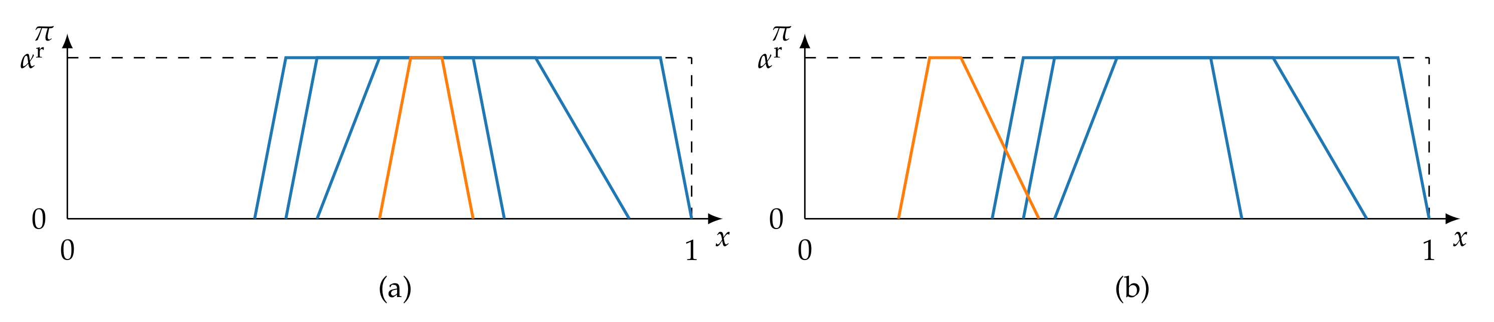
• First, incomplete information and epistemic uncertainty in the training data may lead to assessing a group of sources as consistent prematurely. Information sources may produce different (in)consistent behaviours depending on the training data’s true value and its position on the frame of discernment. Take, for example, a condition-monitoring scenario of a technical system in which sensors state the condition on a discrete frame of discernment $X=\{\mathit{error}\mathit{1},\mathit{error}\mathit{2},\mathit{normal}\}$. Two sensors may both detect two of the conditions (e.g., error1, normal); however, only one is able to detect the third condition (error2). If training data does not include data regarding error2, then with Algorithm 1, both sensors are falsely identified as consistent and grouped into a fusion node. If error2 occurs later, then the sensors behave unexpectedly inconsistently. This problem relates to spurious correlations in probability theory [70], which describes that, in large datasets, it is particularly likely that correlations are found between variables incorrectly.
• Second, defective sources are a cause of unexpected inconsistent behaviour. Defective sources are sources that are trustworthy and therefore have a high reliability but nonetheless start to supply incorrect information [71]. Source defects appear in different forms: Information can change suddenly, drift continuously or incrementally, or can be characterised by an increasing number of outliers [72,73]. Countermeasures are majority-guided fusion rules as applied by Ehlenbröker et al. and Holst and Lohweg [21,23]. This requires redundant and reliable sources in a fusion node.

In the following, we propose three adaptations to the distributed MCS-based fusion topology. These adaptations aim to increase the robustness of the topology in the case of incomplete training data and defective sources.

• Redundancy-Driven Topology Design: To counteract non-representative training data, it must be ensured that information sources are not prematurely deemed to be consistent. For this, it must be analysed whether the consistent behaviour between sources extends over the entire frame of discernment. Therefore, instead of the consistency metric used in (16), the redundancy metric originally proposed in previous works [38,39] is adopted, which ensures that the complete frame of discernment is considered.
• Discounting Defective Sources: Grouping the information sources by consistency (or redundancy) eases the detection of defects [23,24]. Items detected as defective are discounted in the fusion node so that they have less influence on the output of the node. This requires an adjustment of the fusion rule (previously minimum or maximum operator) in the nodes. This defect detection step explicitly exploits the distributed topology to its advantage. This deliberately dismisses the associativity of the overall fusion.
• Estimation-fusion-based Nodes: Averaging information is a natural way to favour opinions of the majority. Adopting estimation fusion in nodes results in more robust behaviour against defects—such as outliers—compared to purely conjunctive fusion as applied in (6).

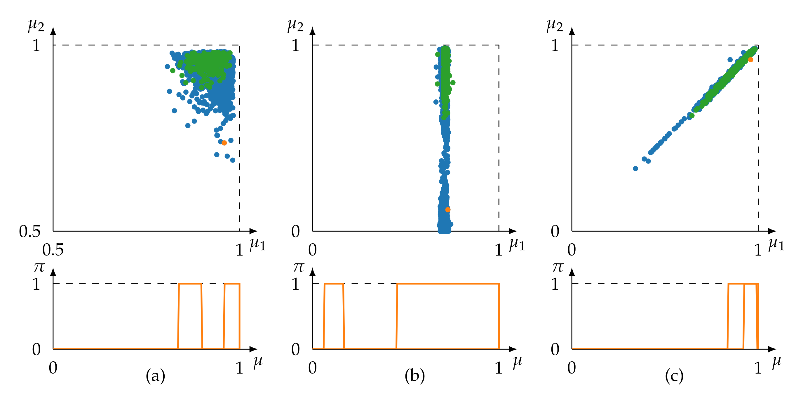
4.3.1. Redundancy-Driven Topology Design

In previous work [39], a redundancy metric was proposed that introduces the notion of range of a set of possibility distributions.

Definition 8

(Range [39]). Given a frame of discernment $X=[x_{\mathrm{a}},x_{\mathrm{b}}]$, the range of a set of possibility distributions $\mathbf{p}$ quantifies how far $\mathbf{p}$ stretches over X. Let $\mathcal{P}(\mathbf{p})$ bet the power set of all possible $\mathbf{p}$, then the range is described by a monotonic increasing function $\mathit{rge}:\mathcal{P}(\mathbf{p})\to [0,1]$ with the following properties:

• Upper bound: If $\mathit{rge}(\mathbf{p})=1$, then $\exists \pi \in \mathbf{p}:\pi (x_{\mathrm{a}})=1$ and $\exists \pi \in \mathbf{p}:\pi (x_{\mathrm{b}})=1$.
• Lower bound: $\mathit{rge}(\mathbf{p})=0$ if $\forall \pi ,{\pi }^{\prime }\in \mathbf{p}:\pi ={\pi }^{\prime }$, i.e., all possibility distributions $\pi \in \mathbf{p}$ are identical.

The range determines whether a set of possibility distributions covers X. Together with the consistency measurement applied in (16), $\mathit{rge}$ is adopted into the topology design approach. Consistency and range are balanced against each other, which results in a dual redundancy metric:

Definition 9

(Possibilistic Redundancy Metric [39]). Let $\mathbf{S}=\{S_1,S_2,\dots ,S_n\}$, i.e., a set of information sources, and $\mathcal{P}(\mathbf{S})$ be all possible combinations of sources, then a possibilistic redundancy metric ρ is a function that maps $\mathcal{P}(\mathbf{S})$ to the unit interval: $\rho :\mathcal{P}(\mathbf{S})\to [0,1]$. Information sources are only redundant if their information items both (i) are redundant themselves and (ii) cover the frame of discernment, i.e., have a high range (Definition 8). In accordance with [39], the redundancy of information items is determined via possibilistic similarity measures. Consistency (2) satisfies the requirements to serve as a similarity measure [32].

In this context and to qualify as an intuitively meaningful metric, the following requirements have to be met:

• Boundaries: A redundancy metric should be able to model complete redundancy and complete non-redundancy. It follows that ρ is minimally and maximally bounded. It is proposed that $\rho \in [0,1]$.
• Identity relation: An information source is fully redundant with identical copies of itself: $\rho (S,S,\dots ,S)=1$. Note that sources can be redundant without necessarily being identical.
• Symmetry: The metric ρ is a symmetric function in all its arguments, i.e.,

  $$\rho (S_1,S_2,\dots ,S_n)=\rho (S_{p\left(1\right)},S_{p\left(2\right)},\dots ,S_{p\left(n\right)})$$
  for any permutation p on ${\mathbb{N}}_{>0}$.

The following relations between redundancy of information items and sources hold.

• If information sources are redundant, then they provide redundant information items. Consequently, $\rho (\mathbf{S})$ increases as the redundancy of information items increase.
• Redundant information items do no necessitate that their information sources are also redundant. Due to cases of incomplete information, redundant information items may be a case of spurious redundancy (similar to spurious correlation).

To capture the idea of a dual metric, $\rho$ is designed to be a function of two pieces of evidence. The evidence against redundancy $e_c:\mathcal{P}(\mathbf{S})\to [0,1]$. As long as information items are redundant, $e_c(\mathbf{S})=0$. Determining the redundancy of information items is both based on the similarity of possibility distributions and related to the notion of possibilistic dependency. An overview of possibilistic redundancy measures for information items is provided by Holst and Lohweg [39]. Dependency measures are reviewed by Dubois et al. [74].

Evidence in favour of redundancy $e_p:\mathcal{P}(\mathbf{S})\to [0,1]$ quantifies the amount of epistemic uncertainty in training data. It incorporates the range of information. It indicates to what degree information is available from the complete frame of discernment. A set of information sources is only redundant if $e_p(\mathbf{S})>0$ and $e_c(\mathbf{S})<1$. The smaller value of $e_p$ and $(1-e_c)$ dominates the redundancy metric. In previous work [39], the geometric mean is proposed as an averaging function for $e_p$ and $e_c$ as follows:

$$\rho (\mathbf{S})=\rho (e_c(\mathbf{S}),e_p(\mathbf{S}))=\sqrt{e_p(\mathbf{S})·\left(1-e_c(\mathbf{S})\right)}.$$

(18)

Let the consistency measure h (2) determine the redundancy between information items and let ${\mathbf{I}}_j$ be the set of information items available at instance j, then

$$e_c(\mathbf{S})=1-\underset{j=\{1,\dots ,m\}}{avg}(h\left({\mathbf{I}}_j\right)),$$

(19)

i.e., $e_c$ averages consistencies available from training data with an averaging operator (see Definition 3). Designing MCS-based topologies (16) is based on the notion that the consistency is above a certain $\alpha$ for all instances. To keep this notion for the redundancy-based design, the minimum operator is used as averaging operator in (19).

The evidence $e_p$ is computed based on the range as follows:

$$e_p(\mathbf{S})=\frac{\mathit{rge}(\mathbf{S})-x_{\mathrm{a}}}{x_{\mathrm{b}}-x_{\mathrm{a}}}.$$

(20)

The range itself is dependent on the position of possibility distributions on the frame of discernment, which is determined by their center of gravity [2]

$$\mathit{pos}(\pi )=\left\{\begin{array}{cc}x\hfill & \mathrm{if}\pi (x)=1\mathrm{and}\forall (x^{\prime })\in \{X\setminus x\}:\pi x^{\prime }=0,\hfill \\ \frac{{\int }_{x_{\mathrm{a}}}^{x_{\mathrm{b}}}x·\pi (x)\mathrm{d}x}{{\int }_{x_{\mathrm{a}}}^{x_{\mathrm{b}}}\pi (x)\mathrm{d}x}\hfill & \mathrm{otherwise}.\hfill \end{array}\right.$$

(21)

The position of a set of possibility distributions $\mathbf{p}$ is obtained by prior disjunctive fusion (5), i.e.,

$$\mathit{pos}(\mathbf{p})=\mathit{pos}(\mathit{fu}(\mathbf{p})).$$

Given a set of information sources $\mathbf{S}=\{S_1,S_2,\dots ,S_n\}$ providing information items ${\mathbf{I}}_j={\mathbf{p}}_j=\{{\pi }_{1,j},{\pi }_{2,j},\dots ,{\pi }_{n,j}\}$, then

$$\mathit{rge}(\mathbf{S})=\underset{j,j^{\prime }\in \{1,\dots ,m\}}{max}\left(|\mathit{pos}({\mathbf{p}}_j)-\mathit{pos}\left({\mathbf{p}}_{j^{\prime }}\right)|\right)=\underset{j\in \{1,\dots ,m\}}{max}(\mathit{pos}({\mathbf{p}}_j))-\underset{j\in \{1,\dots ,m\}}{min}(\mathit{pos}({\mathbf{p}}_j)).$$

(22)

At least one pair ${\mathbf{p}}_j,{\mathbf{p}}_{j^{\prime }}$ of information item sets needs to range over the frame of discernment X in order to provide evidence for a redundant behaviour, i.e., $e_p\mathbf{S}>0$ if $\exists j:\mathit{rge}({\mathbf{p}}_j)>0$.

The redundancy metric $\rho$ (18) is used as a decision criterion to find suitable sets of information sources ${\mathbf{S}}_{\left(k\right)}^{\rho }$ to be fused in fusion nodes ${\mathit{fn}}_{\left(k\right)}$. Algorithm 2 describes a simple approach that searches all subsets of consistency-based fusion nodes in ${\mathcal{S}}_h$ (found by Algorithm 1). A set of sources is only assigned to a fusion node if $\rho \ge \eta$.

Algorithm 2: Algorithm that searches for redundancy-based fusion nodes based on ${\mathcal{S}}_h$ found by Algorithm 1. The algorithm iterates over ${\mathcal{S}}_h$ and searches all ${\mathbf{S}}^{\prime }\subseteq \mathbf{S}$, $\mathbf{S}\in {\mathcal{S}}_h$ for sets meeting the redundancy criterion $\eta$.

As motivated previously, the redundancy-based approach of Algorithm 2 results in a more robust MCS-based topology design than Algorithm 1. As (18) includes the range of information items, the effects of incomplete information and epistemic uncertainty in the training data are reduced. This leads to less detections of spurious relations.

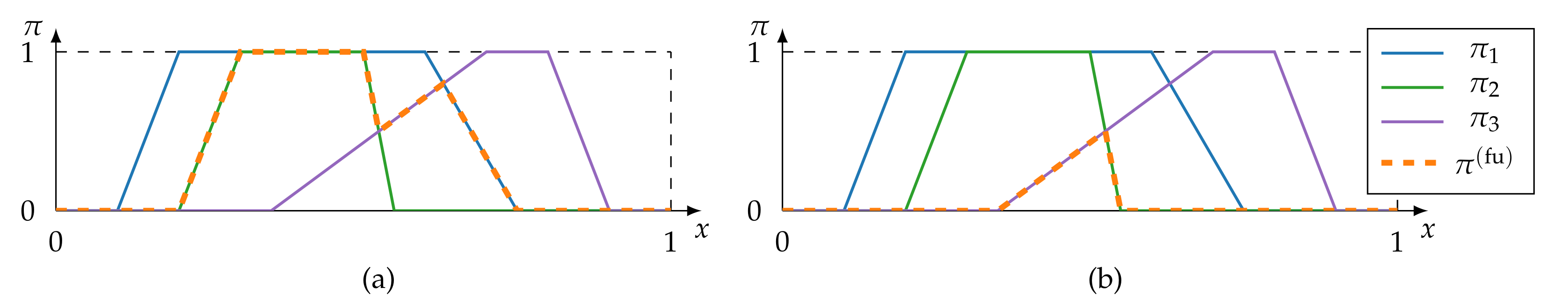
4.3.2. Discounting Defective Sources

Information items that deviate from the expected level of consistency ${\alpha }^{\mathrm{r}}$ (17) are seen as unreliable and, consequently, are discounted in each fusion node. Therefore, the degree of reliability $\mathit{rel}\in [0,1]$ is determined with regard to ${\alpha }^{\mathrm{r}}$. Let $\mathbf{I}$ be information items fused in a node and ${\mathbf{I}}^{*}$ be the largest subset in $\mathbf{I}$, which has (i) $h({\mathbf{I}}^{*})\ge {\alpha }^{\mathrm{r}}$ and (ii) $|{\mathbf{I}}^{*}|>1$; then,

$$(\mathit{rel})I=\left\{\begin{array}{cc}1\hfill & \mathrm{if}h(I,{\mathbf{I}}^{*})>{\alpha }^{\mathrm{r}},\hfill \\ \frac{h(I,{\mathbf{I}}^{*})}{{\alpha }^{\mathrm{r}}}\hfill & \mathrm{if}h(I,{\mathbf{I}}^{*})\le {\alpha }^{\mathrm{r}}.\hfill \end{array}\right.$$

(23)

In the case that there is no unique ${\mathbf{I}}^{*}$ with $h({\mathbf{I}}^{*})\ge {\alpha }^{\mathrm{r}}$ and at least two elements, then all items are seen as fully reliable, and fusion needs to switch to disjunctive fusion.

Information items’ possibility distributions are modified prior to fusion so that they have a lesser effect on the fusion results [4,75]. A modification function for discounting information items has to satisfy the following requirements (extended from previous work [39]).

Definition 10

(Requirements for Information Item Modification). As modification aims at changing fusion outputs, the requirements interact with fusion rules to be applied on π:

• Information preservation: If $\mathit{rel}(I)=1$, then the information must not be changed but instead preserved. Let ${\pi }^{\prime }$ be a modified possibility distribution based on π. If $\mathit{rel}(I)=1$, then ${\pi }^{\prime }=\pi$.
• Neutral element: If $\mathit{rel}(I)=0$, then I needs to have no effect on the fusion. The item I needs to act as a neutral element on fusion operator $\mathit{fu}$, i.e., $\mathit{fu}(I,\mathbf{I})=\mathit{fu}(\mathbf{I})$.
• Monotonicity: For increasing $\mathit{rel}(\mathbf{I})$, I needs to have a monotonic increasing effect on $\mathit{fu}$.

Modification functions were proposed by Yager and Kelman [75]

$${\pi }^{\prime }(x)=\mathit{rel}·\pi (x)+1-\mathit{rel},$$

and Dubois and Prade [4]

$${\pi }^{\prime }(x)=\underset{x\in X}{max}(\pi \left(x\right),1-\mathit{rel}).$$

Both satisfy the requirements for modification only for conjunctive fusion. A general modification function for the use with OWA operators was proposed by Larsen [68]. It is defined based on the andness degree $\mathit{and}\in [0,1]$ of OWA fusion:

$${\pi }^{\prime }(x)=\mathit{and}+\mathit{rel}·((\pi x-\mathit{and})).$$

(24)

The OWA operator results in the minimum fusion for $\mathit{and}=1$ and in maximum fusion for $\mathit{and}=0$. The OWA modification (24) introduces a global possibility level of $\mathit{and}$ to the distribution ${\pi }^{\prime }$. As of this, the modification satisfies the requirement of neutral element only if $\mathit{and}=1$ or $\mathit{and}=0$ but not for $0<\mathit{and}<1$.

All three modification functions raise the overall possibility level globally. As argued in previous work [39], this kind of approach towards modification functions is counterintuitive if it is considered that defective or unreliable sources may err in their estimation of the unknown value v. An unreliable source may be slightly incorrect. Raising the possibility level globally cannot model such a situation. A modification function that widens or shrinks the possibility distribution is proposed as (adapted from previous work [39]):

$$\begin{array}{c}{\pi }^{\prime }(x)=\left\{\begin{array}{cc}{\displaystyle \underset{x^{\prime }\in C}{max}\pi (x^{\prime })}\hfill & \mathrm{if}\mathrm{minimum}\mathrm{fusion},\hfill \\ {\displaystyle \underset{(x^{\prime }(\in C}{min}\pi x^{\prime }}\hfill & \mathrm{if}\mathrm{maximum}\mathrm{fusion},\hfill \end{array}\right.\\ C=\left[x-{(1-\mathit{rel})}^{\beta }·\left(x_{\mathrm{b}}-x_{\mathrm{a}}\right),x+{(1-\mathit{rel})}^{\beta }·\left(x_{\mathrm{b}}-x_{\mathrm{a}}\right)\right],\mathrm{and}\\ X=[x_{\mathrm{a}},x_{\mathrm{b}}].\end{array}$$

(25)

This modification considers both minimum and maximum fusion as they occur in the MCS-based fusion topology but does not approach a global modification. The reliability $\mathit{rel}$ and the control parameter $\beta \in {\mathbb{R}}_{\ge 1}$ define a vicinity around x. The new possibility ${\pi }^{\prime }(x)$ is taken from this vicinity. This creates a widening or shrinking effect, respectively. The parameter $\beta$ allows to control the size of the vicinity and, thus, the extent to which $\mathit{rel}$ alters $\pi (x)$. The larger $\beta$ is, the less effect $\mathit{rel}$ has on $\pi (x)$. If $\mathit{rel}>0$ and $\beta \to \infty$, then (25) has no widening or shrinking effect.

4.3.3. Estimation-Based Fusion Nodes

The third adaptation to increase the robustness of the proposed MCS-based fusion topology is to replace fusion in the first layer (15) with estimation fusion (13). In this way, defective sources have a lesser impact on the fusion result of a node.

Associativity needs to hold for first layer fusion nodes (see Figure 4) if multi-level fusion is to be achieved (splitting fusion nodes into smaller ones). Estimation fusion is only associative if G is associative and monotonic increasing and F is associative. In the proposed estimation-based fusion nodes, G is the minimum operator that satisfies associativity and monotonicity. The function F is defined to be an averaging operator, which is rarely associative, e.g., the arithmetic mean. Multi-level distributed fusion can still be achieved by using a fusion node’s ability to output auxiliary information (see Definition 4).

If a node outputs the number of information items that contributed to its fusion result as a weight w, then a weighted arithmetic mean operator of the form

$$F^{\mathrm{WAM}}(x_1,\dots ,x_n)=\frac{{\sum }_{i=1}^n{w}_i·x_i}{{\sum }_{i=1}^n{w}_i}$$

results in associative fusion. In the following, we refer back to the notation of fusion nodes as defined in Definition 4, i.e., ${\mathbf{I}}_{k,l}$ denotes the set of information items that serve as input to fusion node ${\mathit{fn}}_{(k,l)}$. To achieve associativity, a weight $w_{(k,l)}$ is assigned to the output of ${\mathit{fn}}_{(k,l)}$, which is defined as

$$\begin{array}{c}{w}_{(k,l)}={\displaystyle \sum _{I_{(o,p)}\in {\mathbf{I}}_{(k,l)}}}{w}_{(o,p)}\mathrm{with}\\ w_{(k,1)}=\left|{\mathbf{I}}_{(k,1)}\right|.\end{array}$$

The distributed weighted average function

$$\begin{array}{c}{F}_{(k,l)}^{\mathrm{WAM}}(x_1,\dots ,x_n)={\displaystyle \sum _{I_{(o,p)}\in {\mathbf{I}}_{(k,l)}}}\frac{1}{w_{(o,p)}}{\displaystyle \sum _{I_{(o,p)}\in {\mathbf{I}}_{(k,l)}}}{w}_{(o,p)}·F_{(o,p)}^{\mathrm{WAM}}(x_1,\dots ,x_n)\\ \mathrm{with}{F}_{(k,1)}^{\mathrm{WAM}}(x_1,\dots ,x_n)=\frac{1}{w_{(k,1)}}{\displaystyle \sum _{i=1}^{|I_{(k,1)}|}}{x}_i\end{array}$$

(26)

allows splitting nodes without changing the fusion result. An overview of a distributed fusion topology based on estimation fusion rules is given in Figure 6.

To keep the option of discounting defective sources, weights $w_{(k,l)}$ are modified in the case a defect is detected via (23) as follows:

$$w_{k,l}^{\prime }=w_{k,l}·\mathit{rel}\left(I_{\left(k\right),l}\right).$$

(27)

If $\mathit{rel}\left(I_{\left(k\right),l}\right)=1$, then information is preserved. Otherwise, if $\mathit{rel}\left(I_{\left(k\right),l}\right)=0$ the information item is completely discounted.

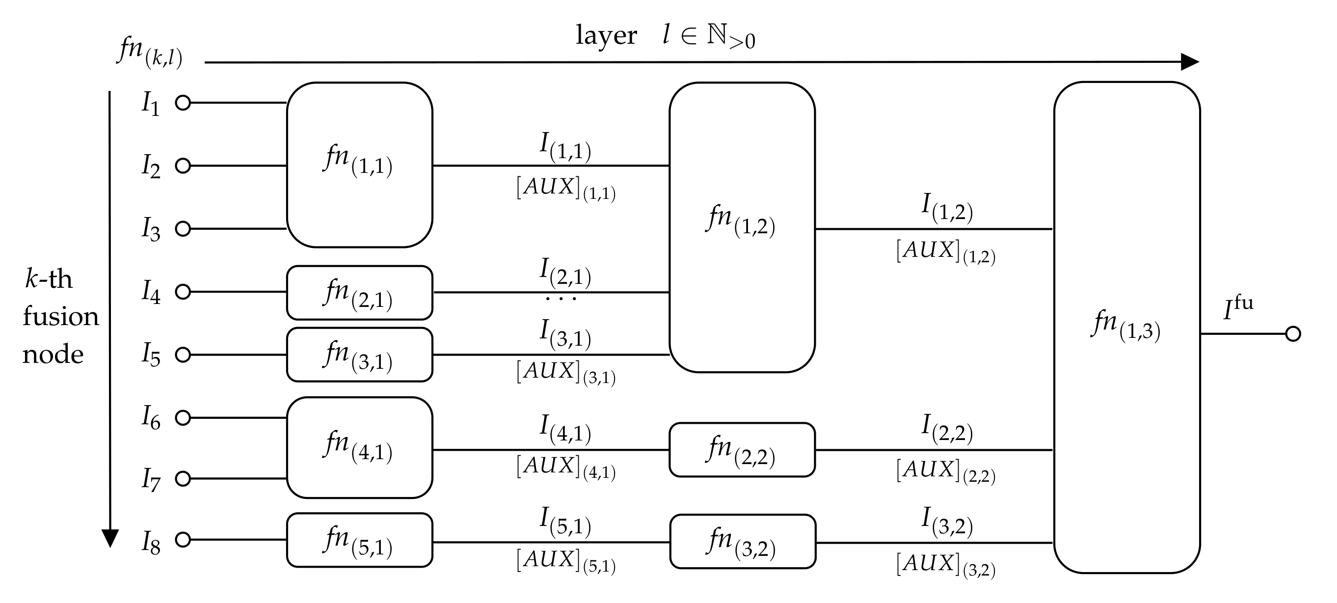
4.4. Remark on Multi-Level Fusion by Splitting Nodes

The MCS-based design approach describes a two-layer fusion topology by first fusing consistent or redundant information items conjunctively and then fusing the intermediate results disjunctively. In this context, multi-layer fusion can be achieved by splitting a single fusion node into multiple smaller ones. This may be beneficial if, e.g., communication or computational loads per node need to be optimised. While this approach of splitting is feasible due to the associativity of applied fusion rules, the ability of the fusion topology to detect and discount defective sources is reduced by doing so.

Discounting information items requires finding the unique largest subset of items whose consistency is greater than ${\alpha }^{\mathrm{r}}$. If multiple sources are defective simultaneously, then—depending on the fusion node size—the largest subset may be made up by defective sources. In the worst case, the maximum number of defective sources a fusion node can handle is $\lfloor \frac{n-1}{2}\rfloor$ [24], with n being the number of sources contributing to a fusion node. As the proposed discounting approach is node-specific, the ability of a node to discount defective sources is hindered by splitting nodes. The smaller n is, the smaller is the maximum number of detectable defective sources. This hast to be kept in mind in designing an MCS-based fusion topology.

5. Evaluation

The evaluation is structured into three parts in which the computational complexity, topology design approaches, and the robustness of distributed MCS fusion are focused. Distributing information fusion is motivated—as outlined in Section 1—by the assumption that computational load per distributed node is less than the load for a single centralised node. First, this assumption is examined for MCS and estimation fusion.

Subsequently, the computational complexity of design Algorithms 1 and 2 are discussed. Their performance and the effectiveness of the MCS-fusion adaptations (see Section 4.3) are then evaluated on selected real-world datasets.

5.1. Computational Complexity

The following evaluation of computational time complexity relies on the Bachmann–Landau notation $f\left(n\right)=\mathcal{O}g\left(n\right)$, which states that a function $f\left(n\right)$ does not grow faster for $n\to \infty$ than $g\left(n\right)$. $f\left(n\right)$ is therefore asymptotically upper bounded by $g\left(n\right)$. $\mathcal{O}g\left(n\right)$ denotes the set of all $f\left(n\right)$ such that there exist positive constants c and $n_0$: $f\left(n\right)\le c·g\left(n\right)$, $\forall n\ge n_0$ [76].

5.1.1. Fusion Rules

In the following, we evaluate whether the computational load of MCS and estimation fusion are decreased by distributing, i.e., whether each fusion node in a distributed topology has a lower load compared to a single centralised node. For MCS fusion, it is assumed that the MCS have already been found, i.e., only (6) is considered.

As (6) consists exclusively of minimum and maximum operations, centralised MCS fusion is $\mathcal{O}(n)$ with n being the number of input information sources. In a distributed two-layer fusion topology, each fusion node has $n_{\mathrm{f}}\le n$ input sources. First layer nodes operate using renormalised minimum fusion; the final layer node applies maximum fusion. Fusion in each node is therefore $\mathcal{O}(n_{\mathrm{f}})$. This simple observation shows that computational load of distributed nodes is less than in centralised fusion—for reasonable MCS fusion topologies.

For estimation fusion, the situation is not as simple. Estimation fusion, as defined in (11), (12), and (13), iterates over every n-tuple $($. Thus, the computational load increases exponentially with its number of inputs n.

Proposition 5.

Let $X^{*}$ be the frame of discernment with the highest cardinality in $\{X_1,\dots ,X_n\}$, then the complexity of estimation fusion rule (11) is $\mathcal{O}(|X^{*}{|}^n·F+|X^{*}{|}^n·G+{\left|X^{*}\right|}^n)$. If G is the minimum operator and F is the arithmetic mean operator, then the complexity is $\mathcal{O}(|X^{*}{|}^n)$.

Proof. 

Equation (11) is a combination of F, G, and the maximum operator. F and G need to be computed for each n-tuple $(x_1,\dots ,x_n)$ for every $x_i\in X_i$, i.e., F and G are computed ${\prod }_{i=1}^n\left|X_i\right|$ times. The maximum operator is computed for each $x\in X$. Its number of inputs is at worst ${\prod }_{i=1}^n\left|X_i\right|$. In total, the complexity of (11) is

$$\begin{array}{cc}\hfill & \mathcal{O}\left(\prod _{i=1}^n|X_i|·F+\prod _{i=1}^n|X_i|·G+\sum _{x\in X}·max)\right)\hfill \\ \hfill =& \mathcal{O}\left(\prod _{i=1}^n|X_i|·F+\prod _{i=1}^n|X_i|·G+\sum _{x\in X}\prod _{i=1}^n|X_i|\right)\hfill \\ \hfill =& \mathcal{O}\left(\prod _{i=1}^n|X_i|·F+\prod _{i=1}^n|X_i|·G+\prod _{i=1}^n|X_i|\right)\hfill \end{array}$$

Let $\mathbf{X}=\{X_1,\dots ,X_n\}$ and $X^{*}={arg\; max}_{X^{\prime }\in \mathbf{X}}\left|X^{\prime }\right|$, then

$$\begin{array}{c}\mathcal{O}(|X^{*}{|}^n·F+|X^{*}{|}^n·G+{\left|X^{*}\right|}^n).\hfill \end{array}$$

With G being the minimum operator and F being the arithmetic mean, this becomes

$$\begin{array}{cc}\mathcal{O}(|X^{*}{|}^n·n+|X^{*}{|}^n·n+{\left|X^{*}\right|}^n)\hfill & \hfill \\ =\mathcal{O}(|X^{*}{|}^n·n)\hfill & \hfill \\ =\mathcal{O}(|X^{*}{|}^n).\hfill & \hfill \end{array}$$

□

Therefore, the complexity of (12) relies on the complexities of G and F; however, it is safe to say that the growth $|X^{*}{|}^n$ leads to issues in practical implementations. Unfortunately, in this case, the lack of scalability cannot be solved by distributing the estimation fusion over several nodes.

Proposition 6.

Let G be the minimum operator and F be an averaging operator as defined in (13). Assume a topology of fusion nodes using estimation fusion (13) exclusively, then fusion at the final fusion node in the last layer still grows exponentially, that is, has $\mathcal{O}({\prod }_{i=1}^n\left|X_i\right|)$ or $\mathcal{O}(|X^{*}{|}^n)$, respectively.

Proof. 

Looking at a single fusion node with $n_k$ inputs, F maps in worst case each tuple $(x_1,\dots ,x_{n_k})$ to a unique point x. Then, the size of the output’s frame of discernment is ${\prod }_{i=1}^{n_k}\left|X_i\right|$. Let ${\mathit{fn}}_{(k,l)}$ be fusion nodes arranged in a topology so that the fusion topology outputs a single information item, i.e., there is a final fusion node ${\mathit{fn}}_{(1,L)}$, $L\in {\mathbb{N}}_{+}$. Assume all n available information items are input into a fusion node exactly once. Then, the final node has to process $2\le n_{\mathrm{final}}\le n$ input information items. The number of tuples to iterate is then ${\prod }_{k=1}^{n_{\mathrm{final}}}\left|X_{k,L-1}\right|$. In a two-layer topology, ${\prod }_{k=1}^{n_{\mathrm{final}}}|X_{k,L-1}|={\prod }_{k=1}^{n_{\mathrm{final}}}{\prod }_{i=1}^{n_k}\left|X_k\right|$. As $n_{\mathrm{final}}={\sum }_{k=1}^{max\left(k\right)}{n}_k$, this is ${\prod }_{i=1}^n|X_i|\le |X^{*}{|}^n$. Thus, fusion at the final node has $\mathcal{O}(|X^{*}{|}^n)$.    □

For estimation fusion, the number of elements in the frame of discernment grows with each fusion node. The final fusion node has to process in worst case $|X^{*}{|}^n$ tuples, which is the same for centralised fusion.

Yager demonstrated [65] that, if all ${\pi }_i$ are convex and if X contains only real-valued ordered elements, then (13) (that is $G=min$ and F is an averaging operator) can also be computed via the crisp-set $\alpha$-cuts

$$A_i^{\alpha }=\{x\in X_i:{\pi }_i(x)\ge \alpha \}\mathrm{with}\alpha \in \left(0,1\right].$$

(28)

Definition 11.

A possibility distribution π is said to be convex iff (1) each of its α-cuts $A^{\alpha }$ are a single closed interval, i.e., $A^{\alpha }=\left[a,b\right]$ and (2) all $A^{\alpha }$ are nested, i.e., $\forall {\alpha }_1>{\alpha }_2:A^{{\alpha }_1}\subseteq A^{{\alpha }_2}$.

For each $\alpha$-level the crisp sets $A_i^{\alpha }$ are fused using the averaging operator F, which results in

$$\begin{array}{cc}\hfill A^{\mathrm{fu}-\alpha }=& F(A_1^{\alpha },\dots ,A_n^{\alpha })\hfill \\ \hfill =& \left[F\left(\underset{x\in A_1^{\alpha }}{min}x,\dots ,\underset{x\in A_n^{\alpha }}{min}x\right),F\left(\underset{x\in A_1^{\alpha }}{max}x,\dots ,\underset{x\in A_n^{\alpha }}{max}x\right)\right].\hfill \end{array}$$

(29)

The fused possibility distribution is then obtained by taking the maximum $\alpha$-level as follows:

$${\pi }^{\left(\mathrm{fu}\right)}(x)=\underset{\alpha }{max}\left\{\begin{array}{cc}\alpha \hfill & \mathrm{if}x\in A^{\mathrm{fu}-\alpha },\hfill \\ 0\hfill & \mathrm{if}x\notin A^{\mathrm{fu}-\alpha }.\hfill \end{array}\right.$$

(30)

Proposition 7.

The computational load of (28)–(30) grows linearly in number of input possibility distributions n, number of elements in $X^{*}$, and number of α-levels $n_{\alpha }$, i.e., (28)–(30) have in total $\mathcal{O}(n·|X^{*}|·n_{\alpha })$.

Proof. 

Equation (28) grows linearly in $|X_i|$. It has to be for each $\alpha$-level and each input possibility distribution, i.e., (28) is $\mathcal{O}(n·|X^{*}|·n_{\alpha })$.

For (29), both minimum and maximum have to be computed n times, F has to be computed two times. This has to be performed for each $\alpha$-level. This results in

$$\begin{array}{cc}\hfill & \mathcal{O}(n_{\alpha }·2·\left(F+n·min+n·max\right))\hfill \\ \hfill =& \mathcal{O}(n_{\alpha }·\left(n+n·|X*|+n·|X^{*}|\right))\hfill \\ \hfill =& \mathcal{O}(n_{\alpha }·n·\left|X^{*}\right|).\hfill \end{array}$$

Equation (28) is a single maximum with $n_{\alpha }$ inputs, i.e., it is $\mathcal{O}(n_{\alpha })$.

In total, (28)–(30) is $\mathcal{O}(n_{\alpha }·n·\left|X^{*}\right|)$.    □

In contrast to (13), the computational load is distributed over fusion nodes if (28)–(30) are distributed. Using $\alpha$-cuts, neither $\left|X\right|$ nor $n_{\alpha }$ grow with each fusion node. Rather, they stay constant. Consequently, increasing the number of fusion nodes in a topology—which decreases the number of inputs per fusion node—reduces the computational load per node. In conclusion, both estimation fusion as well as MCS fusion profit from reduced computational load per node if fusion is distributed.

5.1.2. Fusion Topology Algorithms

Using (16) naively to search all possible subsets of a set of information sources $\mathbf{S}$ for fusion nodes is computationally demanding. Such an approach grows exponentially in number of sources n. The proposed Algorithm 1 presents a computational faster approach.

Proposition 8.

The Algorithm 1 for finding consistency-based fusion nodes has complexity $\mathcal{O}(m·n^2)$ with $n=\left|\mathbf{S}\right|$ and m being the number of training data instances.

Proof. 

Algorithm 1 iterates over all training data instances j. For $j=1$, it searches $\mathbf{S}$ for all MCS. As the algorithm of [58,61] grows linearly in n, this step is $\mathcal{O}(n)$. For each subsequent iteration with $j>1$, it searches all previously MCS found at $j-1$ again for MCS. The maximum number of found MCS is n. The maximum number of sources belonging to an MCS is also n, i.e., each iteration at $j>1$ grows with $n^2$. Consequently, Algorithm 1 is $\mathcal{O}(m·n^2)$.    □

The redundancy-based Algorithm 2 takes the fusion nodes found by Algorithm 1 as input. If an MCS does not meet the redundancy criterion, then Algorithm 2 searches within each MCS for largest subsets with $\rho \ge \eta$.

Proposition 9.

The Algorithm 2 for finding redundancy-based fusion nodes has complexity $\mathcal{O}(2^n)$ with $n=\left|\mathbf{S}\right|$.

Proof. 

Algorithm 2 searches the power set of each MCS ${\mathbf{S}}_{\left(k\right)}^{\mathrm{MCS}-\alpha }$. As the maximum number of sources in ${\mathbf{S}}_{\left(k\right)}^{\mathrm{MCS}-\alpha }$ is n, Algorithm 2 is $\mathcal{O}(2^n)$.    □

In contrast to the consistency-based algorithm, the redundancy-based version scales in its current implementation poorly with number of sources. For reasons of practical implementation, this needs to be addressed in future works. In this regard, plausibility checks are promising as to whether subsets of ${\mathbf{S}}_{\left(k\right)}^{\mathrm{MCS}-\alpha }$ can actually exhibit the required range. In such cases, it would not make sense to search these subsets at all, saving computational time.

5.2. Robustness

Fusion using the default MCS-based topology is prone to unexpected behaviour of information sources regarding their consistency (see Section 4.2). In the following, the MCS fusion design approach and topology are evaluated on selected real-world datasets regarding their robustness. First, consistency-based design is compared to the redundancy-based design approach. Following this, the adaptations of discounting and estimation fusion are evaluated. Implementation and data preprocessing are detailed to increase reproducibility.

5.2.1. Data Preprocessing

Several data preprocessing steps are performed before the implementation. These are necessary (i) to homogenise a heterogeneous frame of discernments, (ii) to reduce the effects of noise (aleatoric uncertainty) on the fusion results and topology design, and (iii) if data are not available as possibility distributions but rather as singular values or probability distributions. Preprocessing comprises the three following steps.

• If data are singular values or probability distributions, they are transferred into possibility distributions first. For this step, singular values x are interpreted as probability distributions with $p(x)=1$ and $x^{\prime }\in X\setminus \left\{x\right\}:p(x^{\prime })=0$. Transformation is conducted by the truncated triangular probability-possibility transformation [49,77,78] resulting in $\pi (x)$.
• Second, sources providing noisy data are regarded as partially unreliable. Their possibility distribution are modified using (25) accordingly. Unreliability values for information sources are determined heuristically.
• Third, modified possibility distributions $\pi x$ are mapped to a common, shared frame of discernment. This X is based on fuzzy memberships $\mu$, i.e., $X=[{\mu }_{\mathrm{a}},{\mu }_{\mathrm{b}}]$. This requires a fuzzy class to be defined to which $\mu (x)$ indicates the degree of membership of x. The class membership function $\mu (x)$ can either be provided by an expert or trained automatically [18,38,39]. Here, $\mu (x)$ is trained by a parametric unimodal potential function proposed proposed by Lohweg et al. [79]:

  $$\begin{array}{c}\mu \left(x\right)=\left\{\begin{array}{c}{2}^{-d(x,{\mathbf{p}}_{\mathrm{l}})}\mathrm{if}x\le \overline{x},\hfill \\ 2^{-d(x,{\mathbf{p}}_{\mathrm{r}})}\mathrm{if}x>\overline{x},\hfill \end{array}\right.\end{array}$$

  (31)

  $$\begin{array}{c}\mathrm{with}d(x,{\mathbf{p}}_{\mathrm{l}})={\left(\frac{\left|x-\overline{x}\right|}{C_{\mathrm{l}}}\right)}^{D_{\mathrm{l}}},\\ d(x,{\mathbf{p}}_{\mathrm{r}})={\left(\frac{\left|x-\overline{x}\right|}{C_{\mathrm{r}}}\right)}^{D_{\mathrm{r}}},\mathrm{and}\end{array}$$

  with $\overline{x}$ being the arithmetic mean of given training data $\mathbf{x}$. The parameters are determined as follows: $C_{\mathrm{l}}=\overline{x}-{min}_{j\in \{1,2,\dots ,m\}}(x_j)$, $C_{\mathrm{r}}={max}_{j\in \{1,2,\dots ,m\}}\left(x_j\right)-\overline{x}$, and $D_{\mathrm{l}}$, $D_{\mathrm{r}}\in {\mathbb{N}}_{>1}$. $D_{\mathrm{l}}$ and $D_{\mathrm{r}}$ are often determined empirically [21,80]. A training routine for $D_{\mathrm{l}}$ and $D_{\mathrm{r}}$ based on density estimations is given by Mönks et al. [81].
  The possibility distribution $\pi (x)$ is then mapped to $\pi (\mu )$ via the extension principle as follows:

  $$\pi (\mu )=\underset{x\in X:\mu (x)=\mu }{max}\pi (x0.$$

A detailed description and visualisations of these preprocessing steps are given previous work [39]. Together, the preprocessing steps allow to apply the proposed design algorithms even on heterogeneous, noisy, and nonpossibilistic data. Robustness against noise can additionally be increased by data filtering. However, since parameters of (31) rely on minimum and maximum values of training data, applying filter directly on training data $\mathbf{x}$ would distort the borders of the unimodal potential function. For this reason, memberships $\mu (x)$—instead of data—are filtered in the preprocessing.

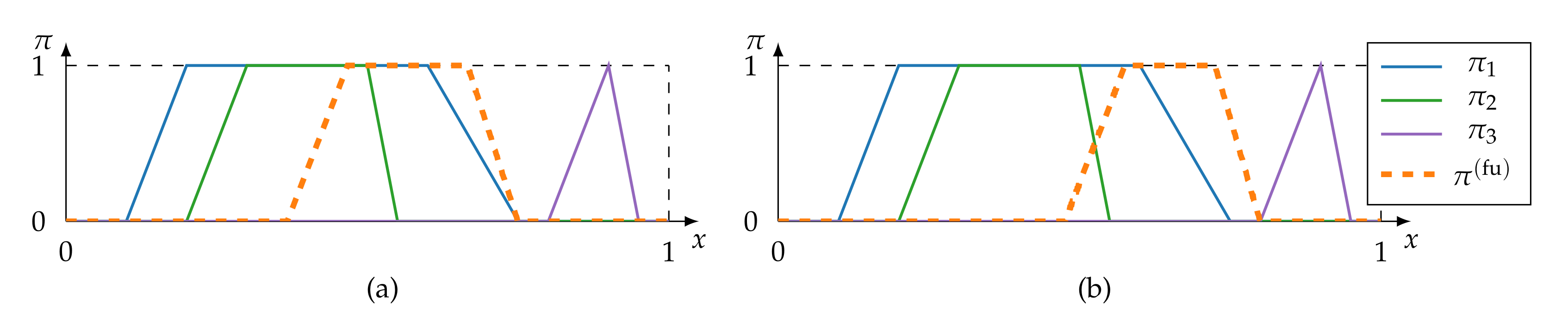
5.2.2. Nonrepresentative Training Data

The effects of nonrepresentative training data on consistency-based MCS topology design and on redundancy-based design are evaluated. Consistency-based topology is obtained by Algorithm 1 with parameter $\alpha =0$ as argued in Proposition 4. Its redundancy-based counterpart is obtained by Algorithm 2. To ensure highly redundant information sources in fusion nodes, parameter $\eta$ is set to $0.6$, i.e., sources are added to a fusion node if their redundancy is greater than or equal to $\eta$.

Both design approaches are applied to the Sensorless Drive Diagnosis (SDD) dataset [82,83]—a multi-class classification dataset (The SDD dataset is available for download at the University of California Machine Learning Repository [84]). Nonrepresentative training data are simulated by withholding data of certain classes from the design algorithms creating a situation of epistemic uncertainty.

For the creation of the Sensorless Drive Diagnostics data set, an electromechanical drive was monitored to detect faulty system behaviour. Data comprise features obtained from phase-related motor currents and voltages. Each feature serves as an information source in this evaluation. The dataset is particularly interesting because (i) it contains highly noisy data and (ii) data are often linearly or non-linearly correlated and thus potentially redundant. The SDD dataset contains 11 classes in total, of which class 1 represents healthy system behaviour (henceforth referred to as the normal condition). All other classes represent various fault states, such as gear or bearing damage.

The design algorithms are executed on two subsets of the dataset. First, only data belonging to the normal condition build a reduced training dataset. This reduced set manifests epistemic uncertainty. It is nonrepresentative with regard to the complete behaviour of information sources. For comparison, the second subset is constructed to include all data, i.e., the complete dataset serves as training data.

Regarding the preprocessing steps, the unimodal potential function (31) is trained on the normal condition with parameters $D_{\mathrm{l}}=2$ and $D_{\mathrm{r}}=2$. To regard the noise in the dataset, possibility distributions are modified with reliability parameters $\forall S\in \mathbf{S}:\mathit{rel}(S)=0.9$ and $\beta =1$. Additionally, memberships are smoothed with a moving average filter using a window size of 5. As the SDD dataset provides data as singular values, the preprocessing steps result in rectangular possibility distributions.

The following behaviour is expected from the topology design approaches, which helps in verifying their output:

• For the consistency-based approach, fusion nodes trained on complete data are expected to be smaller or of equal size compared with nodes trained on reduced data. More specifically, $\forall k,\exists k^{\prime }:{\mathbf{S}}_{\left(k\right),\mathrm{reduced}}^{\mathrm{MCS}-\alpha }\subseteq {\mathbf{S}}_{\left(k^{\prime }\right),\mathrm{complete}}^{\mathrm{MCS}-\alpha }$ because (16) requires consistencies of all data instances to be above the threshold $\alpha$.
• Sources grouped by the redundancy-based approach ${\mathbf{S}}_{\left(k\right)}^{\rho }$ are expected to always be a subset of at least one consistency-based found group ${\mathbf{S}}_{\left(k\right)}^{\mathrm{MCS}-\alpha }$, i.e., $\forall k,\exists k^{\prime }:{\mathbf{S}}_{\left(k\right)}^{\rho }\subseteq {\mathbf{S}}_{\left(k^{\prime }\right)}^{\mathrm{MCS}-\alpha }$ because the redundancy metric (18) is more restrictive than pure consistency. The additional range information (22) prevents sources being added to a fusion node when it is not known that they behave consistently over the complete frame of discernment.

The results of Algorithms 1 and 2 are shown in

Table 2. Fusion nodes and their contributing information sources as designed by Algorithm 1 with parameter $\alpha =0$. Grouped information sources are consistent for all instances of training data (see metric $e_c$ (19)). The left side shows fusion nodes found on reduced, highly epistemic uncertain training data, i.e., only data of the class stating normal condition were available. The right side shows nodes found on complete data. Fusion node sets on reduced training data do not meet the required redundancy threshold (i.e., $\rho \ngeqq \eta$), which is due to the low range-based evidence $e_p$ (20). Information sources are numbered as provided by the SDD dataset [82,83]. Fusion nodes with less than two information sources are omitted. In total, 24 fusion nodes were found on reduced data and 28 on complete data.

Node	Reduced Training Data				Complete Training Data
${\mathit{fn}}_{\left(\mathbf{k}\right)}$	${\mathbf{S}}_{\left(\mathbf{k}\right)},{\mathbf{reduced}}^{\mathbf{MCS}-\alpha }$, $\alpha =\mathbf{0}$	$\rho$	$e_p$	$e_c$	${\mathbf{S}}_{\left(\mathbf{k}\right),\mathbf{complete}}^{\mathbf{MCS}-\alpha }$, $\alpha =\mathbf{0}$	$\rho$	$e_p$	$e_c$
${\mathit{fn}}_{\left(1\right)}$	$\{1,3,25,37\}$	$0.3647$	$0.1330$	0	$\{7,8,9\}$	$0.9919$	$0.9840$	0
${\mathit{fn}}_{\left(2\right)}$	$\{1,5,25,37\}$	$0.4646$	$0.2159$	0	$\{10,11,12\}$	$0.9923$	$0.9847$	0
${\mathit{fn}}_{\left(3\right)}$	$\{1,6,25,37\}$	$0.3460$	$0.1197$	0	$\{13,37\}$	$0.4462$	$0.1991$	0
${\mathit{fn}}_{\left(4\right)}$	$\{1,15,25,28,37,39,40\}$	$0.5329$	$0.2839$	0	$\{16,28,37,40\}$	$0.4043$	$0.1634$	0
${\mathit{fn}}_{\left(5\right)}$	$\{1,25,28,37,39,40,42\}$	$0.5382$	$0.2897$	0	$\{18,41\}$	$0.9513$	$0.9049$	0
${\mathit{fn}}_{\left(6\right)}$	$\{4,28,40\}$	$0.3698$	$0.1368$	0	$\{19,20,21,22,23,24\}$	$0.7830$	$0.6131$	0
${\mathit{fn}}_{\left(7\right)}$	$\{7,8,9,28,40,41\}$	$0.3882$	$0.1507$	0	$\{25,28,37,40,41\}$	$0.4013$	$0.1610$	0
${\mathit{fn}}_{\left(8\right)}$	$\{10,11,12,25,28,37,40\}$	$0.4415$	$0.1950$	0	$\{25,28,37,40,42\}$	$0.4043$	$0.1634$	0
${\mathit{fn}}_{\left(9\right)}$	$\{13,16,25,28,37,40\}$	$0.3863$	$0.1492$	0	$\{31,32,33\}$	$0.8896$	$0.7914$	0
${\mathit{fn}}_{\left(10\right)}$	$\{14,38,39\}$	$0.5450$	$0.2970$	0	$\{34,35,36\}$	$0.9513$	$0.9049$	0
${\mathit{fn}}_{\left(11\right)}$	$\{15,25,28,37,38,39,40\}$	$0.5314$	$0.2824$	0	$\{43,44\}$	$0.8386$	$0.7033$	0
${\mathit{fn}}_{\left(12\right)}$	$\{17,25,37\}$	$0.3657$	$0.1337$	0	$\{46,47,48\}$	$0.7982$	$0.6371$	0
${\mathit{fn}}_{\left(13\right)}$	$\{18,25,28,37,38,39,40,41\}$	$0.3751$	$0.1407$	0	-	-	-	-
${\mathit{fn}}_{\left(14\right)}$	$\{19,20,21,22,23,24,25,28,37,40\}$	$0.3555$	$0.1264$	0	-	-	-	-
${\mathit{fn}}_{\left(15\right)}$	$\{25,27,37,39\}$	$0.3508$	$0.1231$	0	-	-	-	-
${\mathit{fn}}_{\left(16\right)}$	$\{25,28,34,35,36,37,40\}$	$0.3747$	$0.1404$	0	-	-	-	-
${\mathit{fn}}_{\left(17\right)}$	$\{25,28,37,38,39,40,41,42\}$	$0.3234$	$0.1046$	0	-	-	-	-
${\mathit{fn}}_{\left(18\right)}$	$\{25,28,37,39,40,41,42,43,44,45\}$	$0.3545$	$0.1257$	0	-	-	-	-
${\mathit{fn}}_{\left(19\right)}$	$\{25,31,32,33,37\}$	$0.3285$	$0.1079$	0	-	-	-	-
${\mathit{fn}}_{\left(20\right)}$	$\{25,37,46,47,48\}$	$0.2907$	$0.0845$	0	-	-	-	-

and

Table 3. Fusion nodes and their contributing information sources as designed by Algorithm 2 with parameters $\alpha =0$ and $\eta =0.6$. Grouped information sources are consistent for all instances of training data and range over a significant part of the frame of discernment. The left side shows fusion nodes found on reduced, highly epistemic uncertain training data. The right side shows nodes found on complete data. Information sources (features) are numbered as provided by the SDD dataset [82,83]. Fusion nodes with less than two information sources are omitted. In total, 29 fusion nodes were found on reduced data and 31 on complete data.

Node	Reduced Training Data				Complete Training Data
${\mathit{fn}}_{\left(\mathbf{k}\right)}$	${\mathbf{S}}_{\left(\mathbf{k}\right)},{\mathbf{reduced}}^{\mathbf{MCS}-\alpha }$, $\alpha =\mathbf{0}$	$\rho$	$e_p$	$e_c$	${\mathbf{S}}_{\left(\mathbf{k}\right),\mathbf{complete}}^{\mathbf{MCS}-\alpha }$, $\alpha =\mathbf{0}$	$\rho$	$e_p$	$e_c$
${\mathit{fn}}_{\left(1\right)}$	$\{1,15\}$	$0.6239$	$0.3893$	0	$\{7,8,9\}$	$0.9919$	$0.9840$	0
${\mathit{fn}}_{\left(2\right)}$	$\{1,39,42\}$	$0.6228$	$0.3879$	0	$\{10,11,12\}$	$0.8896$	$0.7914$	0
${\mathit{fn}}_{\left(3\right)}$	$\{7,8,9,41\}$	$0.6721$	$0.4517$	0	$\{18,41\}$	$0.9513$	$0.9049$	0
${\mathit{fn}}_{\left(4\right)}$	$\{10,11,12\}$	$0.6302$	$0.3971$	0	$\{19,20,21,22,23,24\}$	$0.7830$	$0.6131$	0
${\mathit{fn}}_{\left(5\right)}$	$\{13,16\}$	$0.6429$	$0.4133$	0	$\{31,32,33\}$	$0.8896$	$0.7914$	0
${\mathit{fn}}_{\left(6\right)}$	$\{14,38,39\}$	$0.6148$	$0.3780$	0	$\{34,35,36\}$	$0.9513$	$0.9049$	0
${\mathit{fn}}_{\left(7\right)}$	$\{19,20,21,22,23,24\}$	$0.6916$	$0.4783$	0	$\{43,44\}$	$0.8386$	$0.7033$	0
${\mathit{fn}}_{\left(8\right)}$	$\{27,39\}$	$0.6415$	$0.4115$	0	$\{46,47,48\}$	$0.7981$	$0.6371$	0
${\mathit{fn}}_{\left(9\right)}$	$\{31,32,33\}$	$0.6367$	$0.4054$	0	-	-	-	-
${\mathit{fn}}_{\left(10\right)}$	$\{34,35,36\}$	$0.6777$	$0.4593$	0	-	-	-	-
${\mathit{fn}}_{\left(11\right)}$	$\{38,42\}$	$0.6077$	$0.3693$	0	-	-	-	-
${\mathit{fn}}_{\left(12\right)}$	$\{39,41,43,44,45\}$	$0.6134$	$0.3763$	0	-	-	-	-
${\mathit{fn}}_{\left(13\right)}$	$\{39,42,43,44,45\}$	$0.6228$	$0.3879$	0	-	-	-	-
${\mathit{fn}}_{\left(14\right)}$	$\{41,42,43,44,45\}$	$0.6100$	$0.3722$	0	-	-	-	-
${\mathit{fn}}_{\left(15\right)}$	$\{46,47,48\}$	$0.6068$	$0.3682$	0	-	-	-	-

, respectively. Both tables show found fusion nodes for the first layer of the two-layer fusion topology. Fusion nodes are shown both for reduced and complete training data along with redundancy $\rho$ (18), range evidence $e_p$ (20), and inconsistency evidence $e_c$ (19).

The results of Table 2 show that the MCS-based topology meets the expectation regarding fusion node sizes. Furthermore, each set ${\mathbf{S}}_{\left(k\right),\mathrm{complete}}^{\mathrm{MCS}-\alpha }$ is a subset of at least one ${\mathbf{S}}_{\left(k\right),\mathrm{reduced}}^{\mathrm{MCS}-\alpha }$, e.g., ${\mathbf{S}}_{\left(1\right),\mathrm{complete}}^{\mathrm{MCS}-\alpha }\subset {\mathbf{S}}_{\left(7\right),\mathrm{reduced}}^{\mathrm{MCS}-\alpha }$. It is also notable that—especially but not exclusively on reduced data—some sources occur in many fusion nodes.

This relates, for example, to sources 25 and 37. Sources with little informative value are likely to be consistent with other sources because such sources provide possibility distributions, which are likely wide or even close to total ignorance. For sources 25 and 37, it is the case that both provide large possibility distributions covering a significant part of the frame of discernment. Lastly, no fusion node based on complete data is exactly similar to fusion nodes based on reduced data (which is different in the following redundancy-based approach). Fusion nodes differ significantly. This means that nonrepresentative data limits the performance of the consistent-based approach substantially, i.e., because epistemic uncertainty is not considered by Algorithm 1 fusion nodes are inflated with spuriously consistent information sources.

The results of the redundancy-based approach (Table 3) also meet the expectations formulated beforehand, i.e., $\forall k,\exists k^{\prime }:{\mathbf{S}}_{\left(k\right)}^{\rho }\subseteq {\mathbf{S}}_{\left(k^{\prime }\right)}^{\mathrm{MCS}-\alpha }$. In contrast to the consistency-based approach, sources with little informative value are not part of fusion nodes (e.g., sources 25 and 37). The computation of the range (22) penalises wide possibility distributions. This is because of the disjunctive fusion prior to computing the position of a set of distributions (21). Sets including information items close to total ignorance are given a position close to $0.5$ resulting in low range values and hence low redundancies.

Similar to the consistency approach, the amount of fusion nodes decreases from reduced to complete training data. This shows that the redundancy-based approach is not able to rule out all sets showing spurious redundancy. However, the majority of nodes learned on complete data are exactly similar to nodes on reduced data. This is true for sets $\{10,11,12\}$, $\{19,20,21,22,23,24\}$, $\{31,32,33\}$, $\{34,35,36\}$, and $\{46,47,48\}$ with $\{7,8,9\}$ coming close. This shows that the redundancy-based approach finds significant sets despite nonrepresentative training data.

Therefore, it copes better than the consistency approach in situations with high epistemic uncertainty because the evidence $e_p$ (20) quantifies epistemic uncertainty. Nonetheless, it is advisable to update and adapt fusion nodes and topology with newly available data. This reduces risk of nodes with spurious redundancy.

Figure 7 depicts scatter plots of selected information sources to visualise the shortcomings of the consistency-based approach and to show the effects of epistemic uncertainty. Information items may be close to each other—and therefore be consistent—for parts of the training data (see plots (a), (b), and (c)). This is indicated by the fact that the positions of items are clustered in the upper right corners for reduced training data. This does not mean that consistent behaviour carries over to complete data (which is only true for (c)).

5.2.3. Defective Sources

Regarding defective sources, two adaptations to the MCS topology were proposed in this paper. Both adaptations—(i) discounting defective sources and (ii) estimation-fusion-based nodes—were evaluated on data with purposely engineered source defects.

The Typical Sensor Defects (TSD) dataset [21] provides such defective sources (The TSD dataset is available for download at https://zenodo.org/record/56358 (accessed on 9 March 2022)). The TSD dataset contains data of a storage container for hazardous and flammable materials measured, e.g., by temperature, smoke, and gas sensors. The dataset comprises several files, which each include a specific simulated source defect, such as incremental drift or outlier readings. For this evaluation, the files “data_standard.csv” and “data_drift_0_001.csv” are used.

The first provides unaltered data without defects. The second one contains the same data with the exception that a temperature sensor (feature 15) drifts with $1‰{\mathrm{h}}^{-1}$ of its base value. Regarding preprocessing, the parameters for the unimodal potential function (31) are provided as metadata in the dataset. As data are hardly affected by noise, sources are fully reliable, and no averaging filter is applied. Data are provided with an error margin of $\pm 2\%$ of the sensor’s measurement range [21] creating a uniform probability density function. Thus, preprocessing results in triangular possibility distributions.

The fusion topology is learned on unaltered data using the consistency-based approach of Algorithm 1—again with $\alpha =0$. This creates three fusion nodes on the first layer:

• ${\mathit{fn}}_{\left(1\right)}$ with ${\mathbf{S}}_{\left(1\right)}^{\mathrm{MCS}-0}=\{17,14,21,16,18,22,12,19,13,11\}$,
• ${\mathit{fn}}_{\left(2\right)}$ with ${\mathbf{S}}_{\left(2\right)}^{\mathrm{MCS}-0}=\{12,15,19,13,11,20\}$, and
• ${\mathit{fn}}_{\left(3\right)}$ with ${\mathbf{S}}_{\left(3\right)}^{\mathrm{MCS}-0}=\{10,9,8,1,2,3,4,5,6,7\}$.

Their fusion results are fused at the final node ${\mathit{fn}}_{(1,2)}$ using MCS fusion (6). For the first layer nodes, the following fusion rules are used and evaluated:

• renormalised conjunctive fusion based on (15),
• discounted renormalised conjunctive fusion extending (15) with (23), (25),
• estimation fusion (13), and
• weighted estimation fusion (27).

Intermediate and final fusion outputs are computed for each of these fusion rules. The results of the same fusion rule on unaltered (standard) and drifted data are compared regarding their similarity. As similarity measure the possibilistic Jaccard index [32,85]

$$\mathit{sim}(\mathbf{p})=\frac{{\int }_0^{1}min\left({\pi }_{\left(k\right),\mathrm{standard}}^{\mathrm{fu}}(\mu ),{\pi }_{\left(k\right),\mathrm{drift}}^{\mathrm{fu}}(\mu )\right)\mathrm{d}x}{{\int }_0^{1}max\left({\pi }_{\left(k\right),\mathrm{standard}}^{\mathrm{fu}}(\mu ),{\pi }_{\left(k\right),\mathrm{drift}}^{\mathrm{fu}}(\mu )\right)\mathrm{d}x}.$$

(32)

is applied. Similarities $\mathit{sim}\in [0,1]$ with $\mathit{sim}=1$ indicating full similarity.

Table 4. Similarity between fusion node outputs on unaltered (standard) dataset and drift affected dataset. The table shows the minimum, arithmetic mean, and maximum of similarities computed on each data instance. The drift affected source belongs to ${\mathit{fn}}_{\left(2\right)}$. Therefore, ${\mathit{fn}}_{\left(1\right)}$ and ${\mathit{fn}}_{\left(3\right)}$ are not explicitly listed. Similarity is increased by proposed countermeasures to defective sources.

Fusion Approach	${\mathit{fn}}_{\left(2\right)}$ Similarity (32)			${\mathit{fn}}_{(1,2)}$ Similarity (32)
	min	mean	max	min	mean	max
Renormalised Conjunctive (15)	$0.0007$	$0.3166$	1	$0.0162$	$0.5335$	1
Discounted Renormalised Conjunctive (15), (23), (25)	0	$0.5064$	1	$0.0162$	$0.6205$	1
Estimation (13)	$0.2686$	$0.6824$	1	$0.1336$	$0.9023$	1
Weighted Estimation (27)	$0.3240$	$0.8051$	1	$0.6288$	$0.9742$	1

lists the minimum, arithmetic mean, and maximum values of the computed similarity values for ${\mathit{fn}}_{\left(2\right)}$ and ${\mathit{fn}}_{(1,2)}$. High similarities show robust behaviour against the defective source. As ${\mathit{fn}}_{\left(1\right)}$ and ${\mathit{fn}}_{\left(3\right)}$ contain no defective sources, they are omitted from the table.

It can be seen from the results that renormalised conjunctive fusion, which is the default rule in MCS fusion, was affected the most by the drifting source. Measures against defective sources are therefore reasonable.

The approach of detecting and discounting by widening inconsistent possibility distributions improved the robustness slightly but not substantially. The ineffectiveness is due to two reasons. First, widening with (25) does shift the fusion result toward reliable sources but does not guarantee that the original fusion result is restored. It is reasonable to assume that parameter $\beta$ has a substantial impact, which needs to be investigated in further works. Second, a drifting possibility distribution may actually drift into other possibility distributions creating a false most consistent subset in the process.

This may lead to situations in which the wrong source is discounted. It is assumed that the risk of this happening decreases with the number of sources in a fusion node. Estimation fusion nodes showed, on the other hand, a significant increase in robustness evidenced by the higher min- and mean-values. Weighted estimation fusion demonstrated the best performance. Due to its averaging nature, estimation fusion reduces the effects of defective sources the better the higher the number of sources.

6. Conclusions

Choosing a topology is one of the main challenges in information fusion system design. Associativity, consistency, and redundancy play key roles in the performance of a topology. In this article, we detailed and discussed a data-driven design approach resulting in a two-layer topology inspired by MCS fusion. Due to the associativity of fusion rules in the first layer nodes, the topology can be extended to multiple layers without affecting the fusion results.

The basic design approach relies on the consistency of information items to find MCS nodes. The resulting consistency-based topology was susceptible to unexpected behaviour from information sources caused by unrepresentative training data or defective sources. We proposed adaptations to the basic design comprising the inclusion of a redundancy metric, the automated discounting of defective sources, and the application of outlier robust estimation fusion.

In the evaluation, we demonstrated that the redundancy-enhanced design resulted in more robust topologies in the case of epistemic uncertainty. Furthermore, evaluation showed that discounting defective sources and estimation fusion reduced the effects of defective sources. Estimation fusion outperformed the discounting approach in this regard mainly because, in certain situations, the discounting approach incorrectly identified sources as defective. Further work is required to improve this.

While the consistency-based approach found MCS in linear time regarding the number of sources and number of data instances, the redundancy-enhanced version searched the power set of all MCS. Although $\forall k:|{\mathbf{S}}_{\left(k\right)}^{\mathrm{MCS}-\alpha }|\le |\mathbf{S}|$ and although, in practical applications, it is reasonable to assume $\forall k:|{\mathbf{S}}_{\left(k\right)}^{\mathrm{MCS}-\alpha }|\ll |\mathbf{S}|$, the scalability of the redundancy-based approach needs to be improved in further works. Another topic that should be addressed in further works is to adapt the design approaches so that they are able to update a topology on streamed data. With new dates becoming available, the epistemic uncertainty is reduced. Updating a topology has the potential to improve the fusion results continuously in small steps.

References

1. Hall, D.L.; Llinas, J.; Liggins, M.E. (Eds.) Handbook of Multisensor Data Fusion: Theory and Practice, 2nd ed.; The Electrical Engineering and Applied Signal Processing Series; CRC Press: Boca Raton, FL, USA, 2009. [Google Scholar]
2. Ayyub, B.M.; Klir, G.J. Uncertainty Modeling and Analysis in Engineering and the Sciences; Chapman & Hall/CRC: Boca Raton, FL, USA, 2006. [Google Scholar]
3. Dubois, D.; Prade, H. On the use of aggregation operations in information fusion processes. Fuzzy Sets Syst. 2004, 142, 143–161. [Google Scholar] [CrossRef] [Green Version]
4. Dubois, D.; Prade, H. Possibility theory in information fusion. In Proceedings of the Third International Conference on Information Fusion, Paris, France, 10–13 July 2000; Volume 1, pp. PS6–PS19. [Google Scholar] [CrossRef]
5. Dubois, D.; Everaere, P.; Konieczny, S.; Papini, O. Main issues in belief revision, belief merging and information fusion. In A Guided Tour of Artificial Intelligence Research: Volume I: Knowledge Representation, Reasoning and Learning; Marquis, P., Papini, O., Prade, H., Eds.; Springer International Publishing: Cham, Switzerland, 2020; pp. 441–485. [Google Scholar] [CrossRef]
6. Dubois, D.; Liu, W.; Ma, J.; Prade, H. The basic principles of uncertain information fusion. An organised review of merging rules in different representation frameworks. Inf. Fusion 2016, 32, 12–39. [Google Scholar] [CrossRef]
7. Varshney, P.K. Multisensor data fusion. Electron. Commun. Eng. J. 1997, 9, 245–253. [Google Scholar] [CrossRef]
8. Mitchell, H.B. (Ed.) Multi-Sensor Data Fusion: An Introduction; Springer: Berlin/Heidelberg, Germany, 2007. [Google Scholar] [CrossRef]
9. Castanedo, F.; Ursino, D.; Takama, Y. A review of data fusion techniques. Sci. World J. 2013, 2013, 704504. [Google Scholar] [CrossRef] [PubMed]
10. Bakr, M.A.; Lee, S. Distributed multisensor data fusion under unknown correlation and data inconsistency. Sensors 2017, 17, 2472. [Google Scholar] [CrossRef] [PubMed] [Green Version]
11. Durrant-Whyte, H.F. Sensor models and multisensor integration. Int. J. Robot. Res. 1988, 7, 97–113. [Google Scholar] [CrossRef]
12. Elmenreich, W. An Introduction to Sensor Fusion; Technical Report; Vienna University of Technology: Vienna, Austria, 2002. [Google Scholar]
13. Elmenreich, W. A review on system architectures for sensor fusion applications. In Software Technologies for Embedded and Ubiquitous Systems; Obermaisser, R., Nah, Y., Puschner, P., Rammig, F.J., Eds.; Springer: Berlin/Heidelberg, Germany, 2007; pp. 547–559. [Google Scholar] [CrossRef] [Green Version]
14. Ben Ayed, S.; Trichili, H.; Alimi, A.M. Data fusion architectures: A survey and comparison. In Proceedings of the 2015 15th International Conference on Intelligent Systems Design and Applications (ISDA), Marrakech, Morocco, 14–16 December 2015; pp. 277–282. [Google Scholar] [CrossRef]
15. Sidek, O.; Quadri, S.A. A review of data fusion models and systems. Int. J. Image Data Fusion 2012, 3, 3–21. [Google Scholar] [CrossRef]
16. Raz, A.K.; Wood, P.; Mockus, L.; DeLaurentis, D.A.; Llinas, J. Identifying interactions for information fusion system design using machine learning techniques. In Proceedings of the 2018 21st International Conference on Information Fusion (FUSION), Cambridge, UK, 10–13 July 2018; pp. 226–233. [Google Scholar] [CrossRef]
17. Luo, R.C.; Kay, M.G. Multisensor integration and fusion in intelligent systems. IEEE Trans. Syst. Man Cybern. 1989, 19, 901–931. [Google Scholar] [CrossRef]
18. Mönks, U. Information Fusion Under Consideration of Conflicting Input Signals. In Technologies for Intelligent Automation; Springer: Berlin/Heidelberg, Germany, 2017. [Google Scholar] [CrossRef]
19. Fritze, A.; Mönks, U.; Holst, C.A.; Lohweg, V. An approach to automated fusion system design and adaptation. Sensors 2017, 17, 601. [Google Scholar] [CrossRef] [Green Version]
20. Rescher, N.; Manor, R. On inference from inconsistent premisses. Theory Decis. 1970, 1, 179–217. [Google Scholar] [CrossRef]
21. Ehlenbröker, J.F.; Mönks, U.; Lohweg, V. Sensor defect detection in multisensor information fusion. J. Sensors Sens. Syst. 2016, 5, 337–353. [Google Scholar] [CrossRef]
22. Holst, C.A.; Lohweg, V. A conflict-based drift detection and adaptation approach for multisensor information fusion. In Proceedings of the 2018 IEEE 23rd International Conference on Emerging Technologies and Factory Automation (ETFA), Turin, Italy, 4–9 September 2018; pp. 967–974. [Google Scholar] [CrossRef]
23. Holst, C.A.; Lohweg, V. Improving majority-guided fuzzy information fusion for Industry 4.0 condition monitoring. In Proceedings of the 2019 22nd International Conference on Information Fusion (FUSION), Ottawa, ON, Canada, 2–5 July 2019. [Google Scholar]
24. Holst, C.A.; Lohweg, V. Feature fusion to increase the robustness of machine learners in industrial environments. Automation 2019, 67, 853–865. [Google Scholar] [CrossRef]
25. Mönks, U.; Lohweg, V.; Dörksen, H. Conflict measures and importance weighting for information fusion applied to Industry 4.0. In Information Quality in Information Fusion and Decision Making; Bossé, É., Rogova, G.L., Eds.; Information Fusion and Data Science; Springer International Publishing: Cham, Switzerland, 2019; pp. 539–561. [Google Scholar] [CrossRef]
26. Fritze, A.; Mönks, U.; Lohweg, V. A support system for sensor and information fusion system design. Procedia Technol. 2016, 26, 580–587. [Google Scholar] [CrossRef]
27. Fritze, A.; Mönks, U.; Lohweg, V. A concept for self-configuration of adaptive sensor and information fusion systems. In Proceedings of the IEEE 21st International Conference on Emerging Technologies and Factory Automation (ETFA), Berlin, Germany, 6–9 September 2016. [Google Scholar] [CrossRef]
28. Boury-Brisset, A.C. Ontology-based approach for information fusion. In Proceedings of the Sixth International Conference of Information Fusion, Cairns, QLD, Australia, 8–11 July 2003; pp. 522–529. [Google Scholar] [CrossRef]
29. Martí, E.; García, J.; Molina, J.M. Adaptive sensor fusion architecture through ontology modeling and automatic reasoning. In Proceedings of the 2015 18th International Conference on Information Fusion (Fusion), Washington, DC, USA, 6–9 July 2015; pp. 1144–1151. [Google Scholar]
30. Steinberg, A.N.; Bowman, C.L. Revisions to the JDL Data Fusion Model. In Handbook of Multisensor Data Fusion; Hall, D.L., Llinas, J., Eds.; The Electrical Engineering and Applied Signal Processing Series; CRC Press: Boca Raton, FL, USA, 2001; pp. 2-1–2-19. [Google Scholar]
31. Smoleń, M.; Augustyniak, P. Assisted living system with adaptive sensor’s contribution. Sensors 2020, 20, 5278. [Google Scholar] [CrossRef] [PubMed]
32. Solaiman, B.; Bossé, É. Possibility Theory for the Design of Information Fusion Systems; Information Fusion and Data Science; Springer International Publishing: Cham, Switzerland, 2019. [Google Scholar]
33. Waltz, E.; Llinas, J. Multisensor Data Fusion; Artech House: Boston, MA, USA, 1990; Volume 685. [Google Scholar]
34. Grabisch, M.; Prade, H. The correlation problem in sensor fusion in a possibilistic framework. Int. J. Intell. Syst. 2001, 16, 1273–1283. [Google Scholar] [CrossRef] [Green Version]
35. Ayoun, A.; Smets, P. Data association in multi-target detection using the transferable belief model. Int. J. Intell. Syst. 2001, 16, 1167–1182. [Google Scholar] [CrossRef]
36. Schubert, J. Clustering belief functions based on attracting and conflicting metalevel evidence using Potts spin mean field theory. Inf. Fusion 2004, 5, 309–318. [Google Scholar] [CrossRef]
37. Schubert, J. Clustering decomposed belief functions using generalized weights of conflict. Int. J. Approx. Reason. 2008, 48, 466–480. [Google Scholar] [CrossRef] [Green Version]
38. Holst, C.A.; Lohweg, V. A redundancy metric based on the framework of possibility theory for technical systems. In Proceedings of the 2020 25th IEEE International Conference on Emerging Technologies and Factory Automation (ETFA), Vienna, Austria, 8–11 September 2020. [Google Scholar] [CrossRef]
39. Holst, C.A.; Lohweg, V. A redundancy metric set within possibility theory for multi-sensor systems. Sensors 2021, 21, 2508. [Google Scholar] [CrossRef]
40. Kamal, A.T.; Bappy, J.H.; Farrell, J.A.; Roy-Chowdhury, A.K. Distributed multi-target tracking and data association in vision networks. IEEE Trans. Pattern Anal. Mach. 2016, 38, 1397–1410. [Google Scholar] [CrossRef] [Green Version]
41. Yoon, K.; Du Kim, Y.; Yoon, Y.C.; Jeon, M. Data association for multi-object tracking via deep neural networks. Sensors 2019, 19, 559. [Google Scholar] [CrossRef] [PubMed] [Green Version]
42. Khaleghi, B.; Khamis, A.; Karray, F.O.; Razavi, S.N. Multisensor data fusion: A review of the state-of-the-art. Inf. Fusion 2013, 14, 28–44. [Google Scholar] [CrossRef]
43. Lohweg, V.; Voth, K.; Glock, S. A possibilistic framework for sensor fusion with monitoring of sensor reliability. In Sensor Fusion; Thomas, C., Ed.; IntechOpen: Rijeka, Croatia, 2011. [Google Scholar] [CrossRef] [Green Version]
44. Zadeh, L.A. Fuzzy sets as a basis for a theory of possibility. Fuzzy Sets Syst. 1978, 1, 3–28. [Google Scholar] [CrossRef]
45. Denœux, T.; Dubois, D.; Prade, H. Representations of uncertainty in artificial intelligence: Probability and possibility. In A Guided Tour of Artificial Intelligence Research: Volume I: Knowledge Representation, Reasoning and Learning; Marquis, P., Papini, O., Prade, H., Eds.; Springer International Publishing: Cham, Switzerland, 2020; pp. 69–117. [Google Scholar] [CrossRef]
46. Salicone, S.; Prioli, M. Measuring Uncertainty within the Theory of Evidence; Springer Series in Measurement Science and Technology; Springer: Cham, Switzerland, 2018. [Google Scholar] [CrossRef]
47. Dubois, D.; Prade, H. Representation and combination of uncertainty with belief functions and possibility measures. Comput. Intell. 1988, 4, 244–264. [Google Scholar] [CrossRef]
48. Dubois, D.; Prade, H. Possibility theory and data fusion in poorly informed environments. Control Eng. Pract. 1994, 2, 811–823. [Google Scholar] [CrossRef]
49. Dubois, D.; Foulloy, L.; Mauris, G.; Prade, H. Probability-possibility transformations, triangular fuzzy sets, and probabilistic inequalities. Reliab. Comput. 2004, 10, 273–297. [Google Scholar] [CrossRef]
50. Yager, R.R. On ordered weighted averaging aggregation operators in multicriteria decisionmaking. IEEE Trans. Syst. Man Cybern. 1988, 18, 183–190. [Google Scholar] [CrossRef]
51. Yager, R.R. On the specificity of a possibility distribution. Fuzzy Sets Syst. 1992, 50, 279–292. [Google Scholar] [CrossRef]
52. Yager, R.R. Measures of specificity. In Computational Intelligence: Soft Computing and Fuzzy-Neuro Integration with Applications; Kaynak, O., Zadeh, L.A., Türkşen, B., Rudas, I.J., Eds.; Springer: Berlin/Heidelberg, Germany, 1998; pp. 94–113. [Google Scholar]
53. Yager, R.R. Measures of specificity over continuous spaces under similarity relations. Fuzzy Sets Syst. 2008, 159, 2193–2210. [Google Scholar] [CrossRef]
54. Yager, R.R. Aggregation operators and fuzzy systems modeling. Fuzzy Sets Syst. 1994, 67, 129–145. [Google Scholar] [CrossRef]
55. Zadeh, L.A. The concept of a linguistic variable and its application to approximate reasoning—II. Inf. Sci. 1975, 8, 301–357. [Google Scholar] [CrossRef]
56. Klement, E.P. Triangular Norms; Springer eBook Collection Mathematics and Statistics; Springer: Dordrecht, Germany, 2000; Volume 8. [Google Scholar] [CrossRef]
57. Benferhat, S.; Dubois, D.; Prade, H. Reasoning in inconsistent stratified knowledge bases. In Proceedings of the 26th IEEE International Symposium on Multiple-Valued Logic (ISMVL’96), Compostela, Spain, 29–31 May 1996; pp. 184–189. [Google Scholar] [CrossRef]
58. Dubois, D.; Fargier, H.; Prade, H. Multi-source information fusion: A way to cope with incoherences. In Proceedings of the French Days on Fuzzy Logic and Applications (LFA), Paris, France, 21 October 2000; pp. 123–130. [Google Scholar]
59. Liu, W.; Qi, G.; Bell, D.A. Adaptive merging of prioritized knowledge bases. Fundam. Inform. 2006, 73, 389–407. [Google Scholar]
60. Hunter, A.; Liu, W. A context-dependent algorithm for merging uncertain information in possibility theory. IEEE Trans. Syst. Man Cybern. Part A Syst. Hum. 2008, 38, 1385–1397. [Google Scholar] [CrossRef]
61. Destercke, S.; Dubois, D.; Chojnacki, E. Possibilistic information fusion using maximal coherent subsets. IEEE Trans. Fuzzy Syst. 2009, 17, 79–92. [Google Scholar] [CrossRef] [Green Version]
62. Yager, R.R. Aggregating evidence using quantified statements. Inf. Sci. 1985, 36, 179–206. [Google Scholar] [CrossRef]
63. Dubois, D.; Prade, H.; Testemale, C. Weighted fuzzy pattern matching. Fuzzy Sets Syst. 1988, 28, 313–331. [Google Scholar] [CrossRef]
64. Oussalah, M.; Maaref, H.; Barret, C. From adaptive to progressive combination of possibility distributions. Fuzzy Sets Syst. 2003, 139, 559–582. [Google Scholar] [CrossRef]
65. Yager, R.R. A general approach to the fusion of imprecise information. Int. J. Intell. Syst. 1997, 12, 1–29. [Google Scholar] [CrossRef]
66. Zadeh, L.A. Fuzzy sets. Inf. Control 1965, 8, 338–353. [Google Scholar] [CrossRef] [Green Version]
67. Glock, S.; Voth, K.; Schaede, J.; Lohweg, V. A framework for possibilistic multi-source data fusion with monitoring of sensor reliability. In Proceedings of the World Conference on Soft Computing, San Francisco, CA, USA, 23–26 May 2011. [Google Scholar]
68. Larsen, H.L. Efficient importance weighted aggregation between min and max. In Proceedings of the ninth Conference on Information Processing and Management of Uncertainty in Knowledge-based Systems, Annecy, France, 1–5 July 2002; pp. 1203–1208. [Google Scholar]
69. Oussalah, M. Study of some algebraical properties of adaptive combination rules. Fuzzy Sets Syst. 2000, 114, 391–409. [Google Scholar] [CrossRef]
70. Calude, C.; Longo, G. The deluge of spurious correlations in big data. Found. Sci. 2017, 22, 595–612. [Google Scholar] [CrossRef] [Green Version]
71. Delmotte, F.; Borne, P. Modeling of reliability with possibility theory. IEEE Trans. Syst. Man Cybern. Part A Syst. Hum. 1998, 28, 78–88. [Google Scholar] [CrossRef]
72. Žliobaitė, I. Learning under concept drift: An overview. arXiv 2010, arXiv:1010.4784. [Google Scholar] [CrossRef]
73. Ramírez-Gallego, S.; Krawczyk, B.; García, S.; Woźniak, M.; Herrera, F. A survey on data preprocessing for data stream mining: Current status and future directions. Neurocomputing 2017, 239, 39–57. [Google Scholar] [CrossRef]
74. Dubois, D.; Del Cerro, L.F.; Herzig, A.; Prade, H. An ordinal view of independence with application to plausible reasoning. In Uncertainty Proceedings 1994; Mantaras, R.L.d., Poole, D., Eds.; Morgan Kaufmann: Burlington, MA, USA, 1994; pp. 195–203. [Google Scholar] [CrossRef] [Green Version]
75. Yager, R.R.; Kelman, A. Fusion of fuzzy information with considerations for compatibility, partial aggregation, and reinforcement. Int. J. Approx. Reason. 1996, 15, 93–122. [Google Scholar] [CrossRef] [Green Version]
76. Knuth, D.E. Big omicron and big omega and big theta. ACM Sigact News 1976, 8, 18–24. [Google Scholar] [CrossRef]
77. Lasserre, V.; Mauris, G.; Foulloy, L. A simple possibilistic modelisation of measurement uncertainty. In Uncertainty in Intelligent and Information Systems; Bouchon-Meunier, B., Yager, R.R., Zadeh, L.A., Eds.; World Scientific Publishing Co. Pte. Ltd.: Singapore, 2000; Volume 20, pp. 58–69. [Google Scholar] [CrossRef]
78. Mauris, G.; Lasserre, V.; Foulloy, L. Fuzzy modeling of measurement data acquired from physical sensors. IEEE Trans. Instrum. Meas. 2000, 49, 1201–1205. [Google Scholar] [CrossRef]
79. Lohweg, V.; Diederichs, C.; Müller, D. Algorithms for hardware-based pattern recognition. EURASIP J. Appl. Signal Process. 2004, 2004, 1912–1920. [Google Scholar] [CrossRef] [Green Version]
80. Voth, K.; Glock, S.; Mönks, U.; Lohweg, V.; Türke, T. Multi-sensory machine diagnosis on security printing machines with two-layer conflict solving. In Proceedings of the SENSOR+TEST Conference 2011, Nuremberg, Germany, 7–9 June 2011; pp. 686–691. [Google Scholar] [CrossRef]
81. Mönks, U.; Petker, D.; Lohweg, V. Fuzzy-Pattern-Classifier training with small data sets. In Information Processing and Management of Uncertainty in Knowledge-Based Systems. Theory and Methods; Hüllermeier, E., Kruse, R., Hoffmann, F., Eds.; Springer: Berlin/Heidelberg, Germany, 2010; pp. 426–435. [Google Scholar] [CrossRef]
82. Paschke, F.; Bayer, C.; Bator, M.; Mönks, U.; Dicks, A.; Enge-Rosenblatt, O.; Lohweg, V. Sensorlose Zustandsüberwachung an Synchronmotoren. In 23. Workshop Computational Intelligence; Hoffmann, F., Hüllermeier, E., Mikut, R., Eds.; KIT Scientific Publishing: Karlsruhe, Germany, 2013; Volume 46, pp. 211–225. [Google Scholar]
83. Lessmeier, C.; Enge-Rosenblatt, O.; Bayer, C.; Zimmer, D. Data acquisition and signal analysis from measured motor currents for defect detection in electromechanical drive systems. In Proceedings of the PHM Society European Conference, Nantes, France, 8–10 July 2014. [Google Scholar] [CrossRef]
84. Dua, D.; Graff, C. UCI Machine Learning Repository; University of California, School of Information and Computer Science: Irvine, CA, USA, 2020; Available online: http://archive.ics.uci.edu/ml (accessed on 14 March 2022).
85. Charfi, A.; Bouhamed, S.A.; Bossé, É.; Kallel, I.K.; Bouchaala, W.; Solaiman, B.; Derbel, N. Possibilistic similarity measures for data science and machine learning applications. IEEE Access 2020, 8, 49198–49211. [Google Scholar] [CrossRef]
86. Higashi, M.; Klir, G.J. Measures of uncertainty and information based on possibility distributions. Int. J. Gen. Syst. 1982, 9, 43–58. [Google Scholar] [CrossRef]
87. Higashi, M.; Klir, G.J. On the notion of distance representing information closeness: Possibility and probability distributions. Int. J. Gen. Syst. 1983, 9, 103–115. [Google Scholar] [CrossRef]
Figure 1. Three example information fusion topologies. (a) Centralised fusion, (b) serial fusion, and (c) hierarchical fusion.
Metrology 02 00012 g001
Figure 2. An example of the interaction between estimation fusion (12) and X as discussed in Proposition 1. A frame of discernment X = [ 0 , 10 ] and three possibility distributions are given. Each possibility distribution claims complete knowledge; π 1 ( x = 3 ) = 1 , π 2 ( x = 5 ) = 1 , and π 3 ( x = 7 ) = 1 . The plots show fusion results (dashed red) in which F is the arithmetic mean and G is (a) the minimum, (b) the maximum, and (c) the arithmetic mean operator.
Metrology 02 00012 g002
Figure 3. An example for a three-layer fusion topology. Fusion nodes are denoted with fn ( k , l ) and their output information items with I ( k , l ) together with auxiliary information [ AUX ] ( k , l ) . The index l denotes the layer. Within a layer l, the nodes are numbered consecutively by k.
Metrology 02 00012 g003
Figure 4. An example of a MCS-based fusion topology. Depicted are seven information sources fused in a two-layer topology. On the left side (a), the topology itself is shown with minimum fusion on the first layer and maximum fusion on the second layer. The right side (b) illustrates the associated possibility distributions from which the topology is constructed.
Metrology 02 00012 g004
Figure 5. Information items of a fusion node with consistency level α r = 1 . Left plot (a) shows possibility distributions with expected consistent behaviour. In the right side plot (b), a single defective information item with unexpected behaviour (marked in red) causes h ( I ) < α r . Fusion with (15) results in dissimilar possibility distributions.
Metrology 02 00012 g005
Figure 6. Example of an MCS-based fusion topology adapted with weighted estimation fusion. Previously conjunctive fusion nodes (first level fusion; see also Figure 4) are replaced with the estimation fusion rule described by (13). To preserve the associativity of the first level fusion nodes, the weighted averaging operator F WAM described by (26) is applied as function F. If the estimation-based nodes are split into a multi-level topology, then F WAM requires fusion nodes to communicate the number of input information items.
Metrology 02 00012 g006
Figure 7. Information items of selected information sources belonging to reduced training data (green) and complete training data (blue). Data belongs to the Sensorless Drive Diagnosis dataset [82,83]. Subplot (a) shows information sources (features) { 1 , 5 } , (b) { 25 , 10 } , and (c) { 43 , 45 } . Each point in the scatter plots represents the position or centre of gravity of a possibility distribution obtained by (21). Possibility distributions of a single pair are plotted below each scatter plot to give an intuition about the size of the distributions. In the case of reduced training data, information sources (a) { 1 , 5 } and (b) { 25 , 10 } belong to fusion nodes in the consistency-based approach (see Table 2) but not in the redundancy-based approach (see Table 3). Without the additional information provided by the range metric (22), the consistency-based approach considers sources, which result in being inconsistent on complete training data. Sources (c) { 43 , 45 } are given as an example in which information items are consistent over the complete training data. Both the consistency-based as well as the redundancy-based approach consider { 43 , 45 } in fusion nodes. Note that the scatter plot in (a) is zoomed in for better visibility.
Metrology 02 00012 g007