
Effect of a Misidentified Centre of a Type ASG Material Measure on the Determined Topographic Spatial Resolution of an Optical Point Sensor


Abstract
:1. Introduction and Literature Review
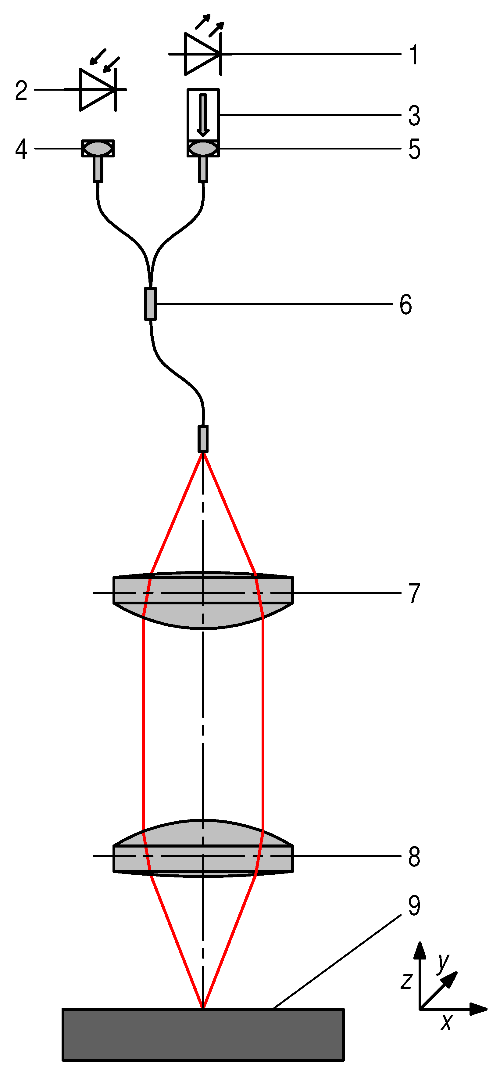
2. Setup
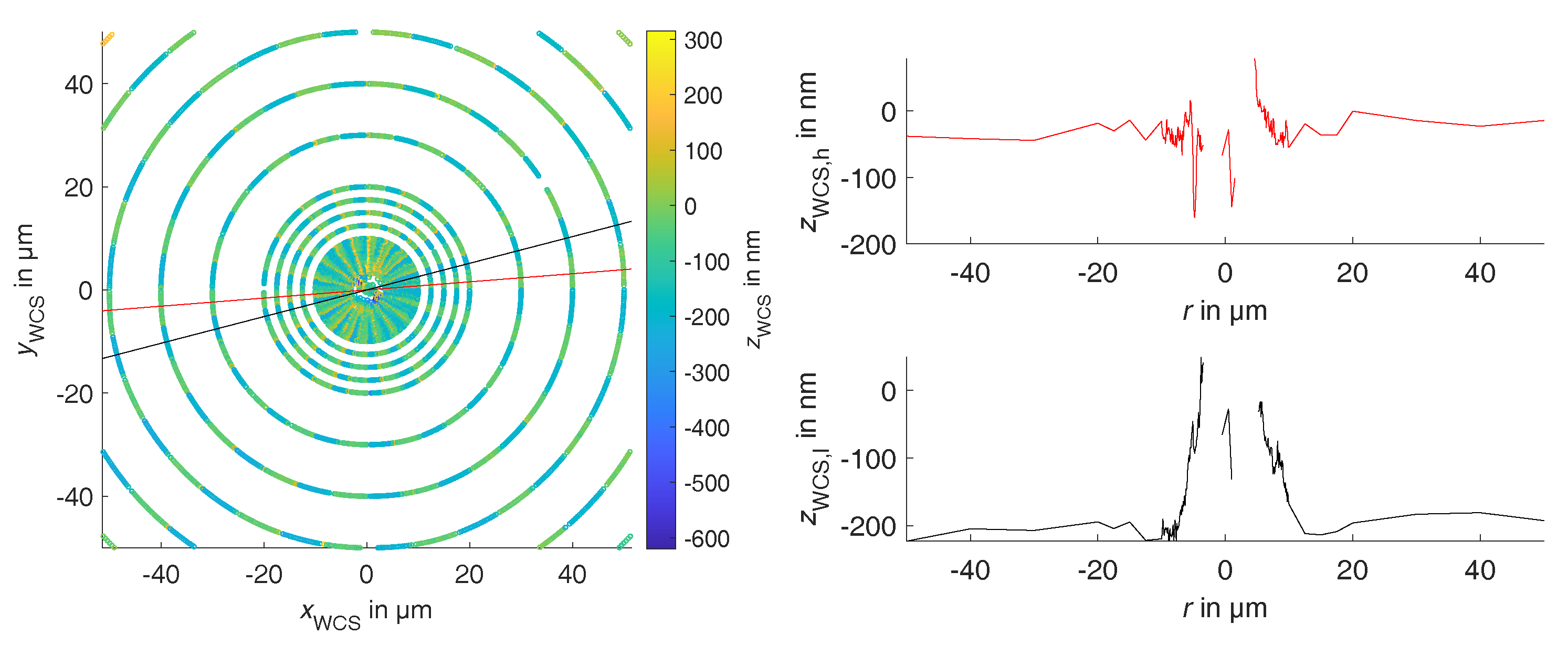
3. Determination of the Workpiece Coordinate System
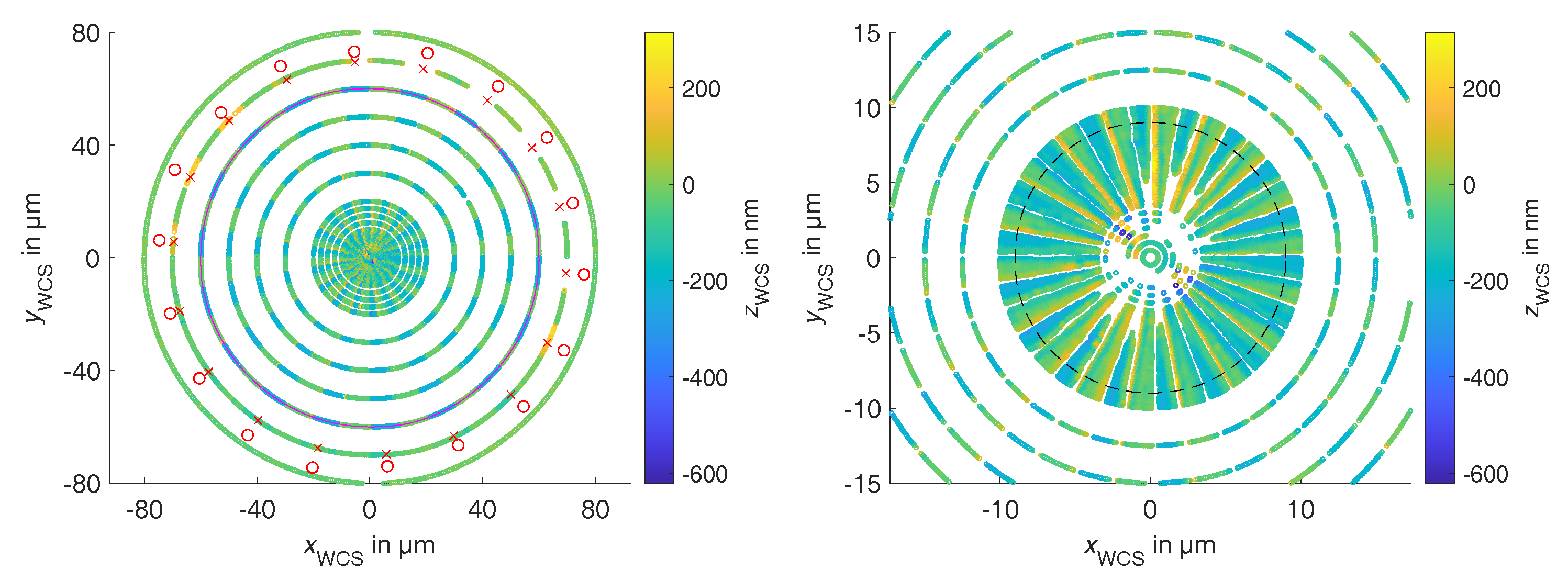
4. Radial Measurement and Evaluation of
5. Measurement and Evaluation of according to the NPL Good Practice Guide
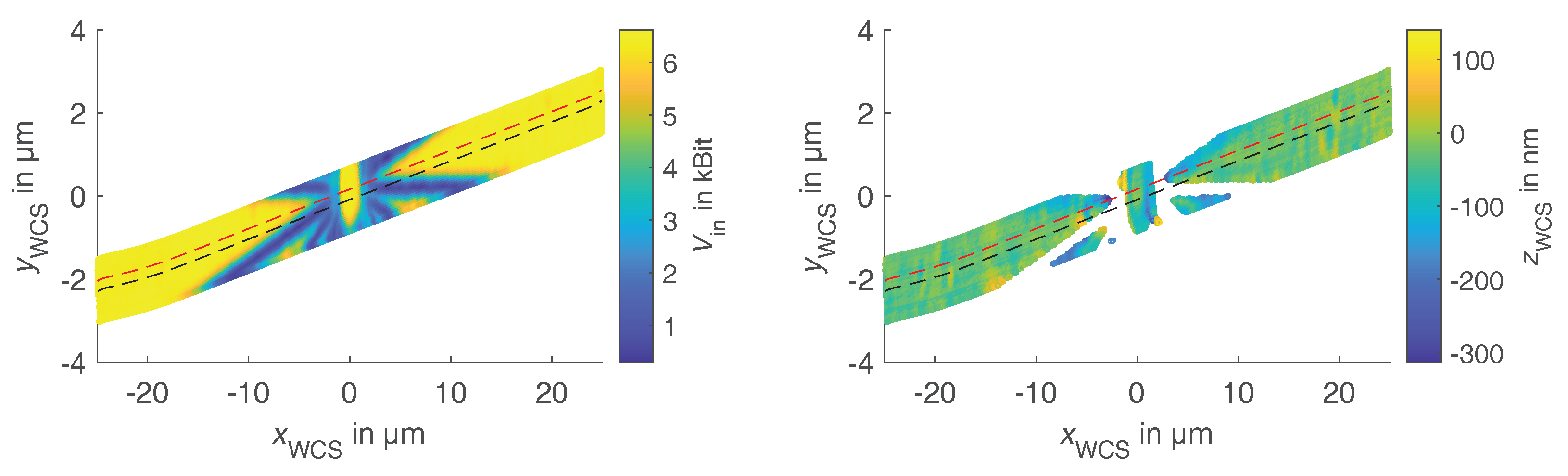
5.1. Evaluation of the Areal Measurement according to the NPL Good Practice Guide
5.2. Measurement and Evaluation according to the NPL Good Practice Guide
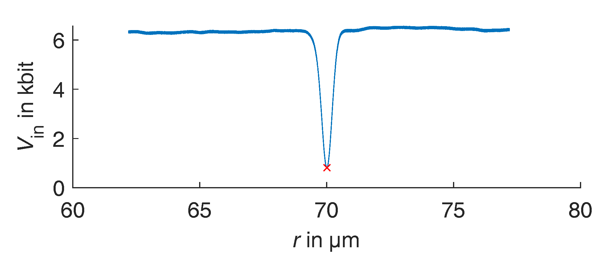
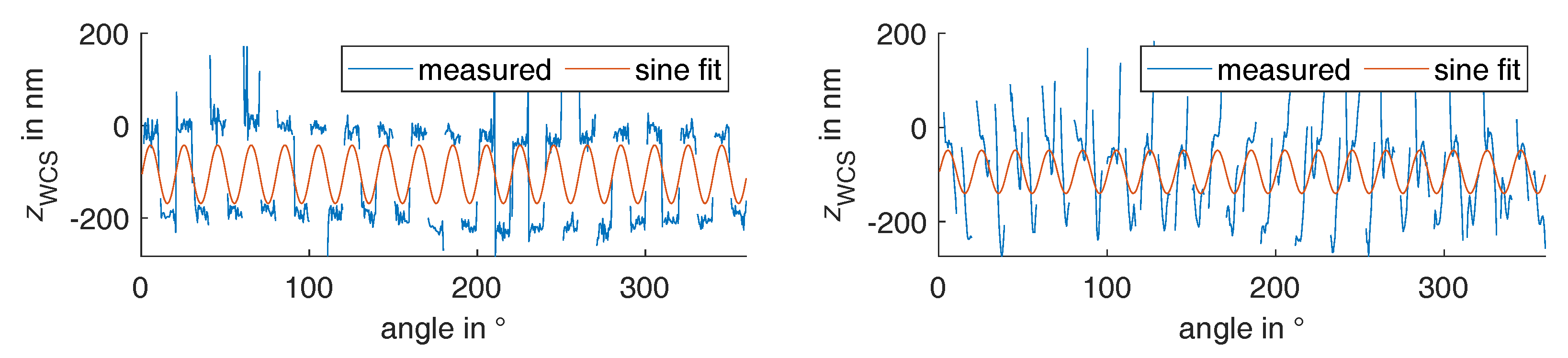
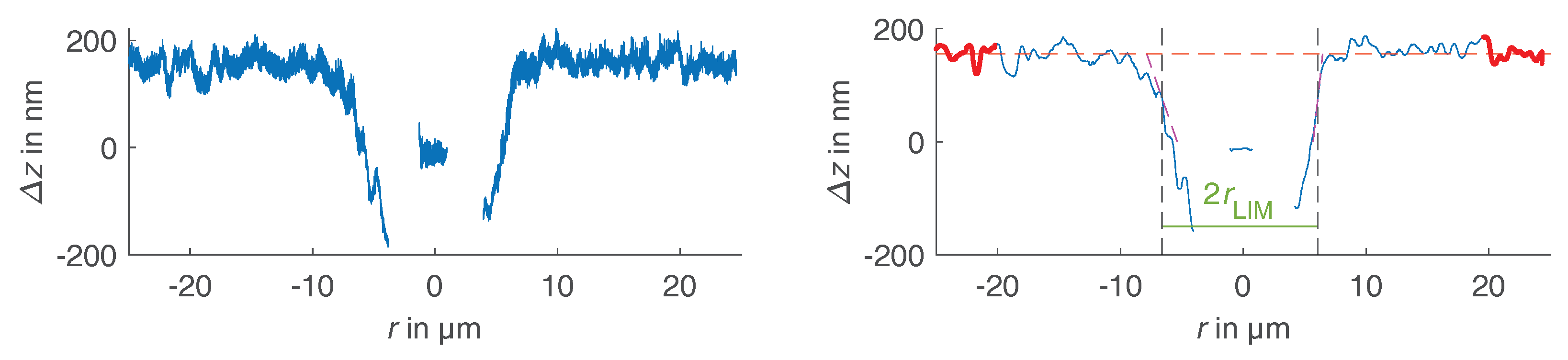
5.3. Effect of a Misidentified Target Centre
5.4. Modified Good Practice Guide
- Roughly determine the centre of the Siemens star.
- Conduct a radial measurement on a radius where the structures are well resolvable.
- Calculate the phase of the structures by a Fourier series approximation of this radial measurement.
- Conduct several parallel line scans with a small offset in the direction of the phase of the structures in a groove and on an adjacent top level.
- Determine the line scans going through the centre of the Siemens star by finding, for the scans both in a groove and on an adjacent top level, the one with the smallest when evaluating the unprocessed raw signal, for instance, of the photodetector, not the topographic data.
- Calculate with the topographic data of the two line scans that go through the centre of the Siemens star. An appropriate low-pass filter should be applied to reduce the noise level of the data.
6. Summary
7. Conclusions
Author Contributions
Funding
Institutional Review Board Statement
Informed Consent Statement
Data Availability Statement
Acknowledgments
Conflicts of Interest
References
- Bruzzone, A.A.G.; Costa, H.L.; Lonardo, P.M.; Lucca, D.A. Advances in engineered surfaces for functional performance. CIRP Ann. 2008, 57, 750–769. [Google Scholar] [CrossRef]
- Zhang, S.; Zhou, Y.; Zhang, H.; Xiong, Z.; To, S. Advances in ultra-precision machining of micro-structured functional surfaces and their typical applications. Int. J. Mach. Tools Manuf. 2019, 142, 16–41. [Google Scholar] [CrossRef]
- Blondiaux, N.; Diserens, M.; Chauvy, P.F.; Oudot, B.; Pugin, R. Manufacturing of hierarchically structured surfaces for decorative applications. In Proceedings of the Euspen’s 21st International Conference & Exhibition, Copenhagen, Denmark, 7–10 June 2021; pp. 119–120. [Google Scholar]
- Leach, R. Introduction to Surface Texture Measurement. In Optical Measurement of Surface Topography, 1st ed.; Leach, R., Ed.; Springer: Berlin/Heidelberg, Germany, 2011; Chapter 1; pp. 1–15. [Google Scholar]
- Jiang, X.J.; Whitehouse, D.J. Technological shifts in surface metrology. CIRP Ann. 2012, 61, 815–836. [Google Scholar] [CrossRef]
- Leach, R.; Ferrucci, M.; Haitjema, H. Dimensional Metrology. In CIRP Encyclopedia of Production Engineering; Springer: Berlin/Heidelberg, Germany, 2019; pp. 1–11. [Google Scholar]
- Joint Committee for Guides in Metrology. JCGM 100:2008. Evaluation of Measurement Data—Guide to the Expression of Uncertainty in Measurement. 2008. Available online: https://www.bipm.org/documents/20126/2071204/JCGM_100_2008_E.pdf/cb0ef43f-baa5-11cf-3f85-4dcd86f77bd6 (accessed on 1 October 2021).
- Haitjema, H. Measurement Uncertainty. In CIRP Encyclopedia of Production Engineering; Laperrière, L., Reinhart, G., Eds.; Springer: Berlin/Heidelberg, Germany, 2014; pp. 852–857. [Google Scholar]
- Whitehouse, D.J. Comparison Between Stylus and Optical Methods for Measuring Surfaces. CIRP Ann. 1988, 37, 649–653. [Google Scholar] [CrossRef]
- Weckenmann, A.; Estler, T.; Peggs, G.; McMurtry, D. Probing Systems in Dimensional Metrology. CIRP Ann. 2004, 53, 657–684. [Google Scholar] [CrossRef]
- Leach, R.K.; Giusca, C.L.; Naoi, K. Development and characterization of a new instrument for the traceable measurement of areal surface texture. Meas. Sci. Technol. 2009, 20, 125102. [Google Scholar] [CrossRef]
- Thomsen-Schmidt, P. Characterization of a traceable profiler instrument for areal roughness measurement. Meas. Sci. Technol. 2011, 22, 094019. [Google Scholar] [CrossRef]
- Nouira, H.; Salgado, J.A.; El-Hayek, N.; Ducourtieux, S.; Delvallée, A.; Anwer, N. Setup of a high-precision profilometer and comparison of tactile and optical measurements of standards. Meas. Sci. Technol. 2014, 25, 044016. [Google Scholar] [CrossRef] [Green Version]
- Binnig, G.; Quate, C.F.; Gerber, C. Atomic Force Microscope. Phys. Rev. Lett. 1986, 56, 930–933. [Google Scholar] [CrossRef] [PubMed] [Green Version]
- Meyer, G.; Amer, N.M. Optical-beam-deflection atomic force microscopy: The NaCl (001) surface. Appl. Phys. Lett. 1990, 56, 2100–2101. [Google Scholar] [CrossRef]
- Giessibl, F.J.; Gerber, C.; Binnig, G. A low-temperature atomic force/scanning tunneling microscope for ultrahigh vacuum. J. Vac. Sci. Technol. B 1990, 9, 984–988. [Google Scholar] [CrossRef] [Green Version]
- Danzebrink, H.U.; Pohlenz, F.; Dai, G.; Dal Savio, C. Metrological Scanning Probe Microscope—Instruments for Dimensional Nanometrology. In Nanoscale Calibration Standards and Methods: Dimensional and Related Measurements in the Micro-and Nanometer Range, 1st ed.; Wilkening, G., Koenders, L., Eds.; Wiley-VCH: Hoboken, NJ, USA, 2005; pp. 3–21. [Google Scholar]
- Lonardo, P.M.; Lucca, D.A.; De Chiffre, L. Emerging Trends in Surface Metrology. CIRP Ann. 2002, 51, 701–723. [Google Scholar] [CrossRef]
- Schwenke, H.; Neuschaefer-Rube, U.; Pfeifer, T.; Kunzmann, H. Optical Methods for Dimensional Metrology in Production Engineering. CIRP Ann. 2002, 51, 685–699. [Google Scholar] [CrossRef]
- Gao, W.; Haitjema, H.; Fang, F.Z.; Leach, R.K.; Cheung, C.F.; Savio, E.; Linares, J.M. On-machine and in-process surface metrology for precision manufacturing. CIRP Ann. 2019, 68, 843–866. [Google Scholar] [CrossRef] [Green Version]
- Schmitt, R.; Damm, B. Maschinenintegrierte Messtechnik. In Koordinatenmesstechnik—Flexible Strategien für Funktions- und Fertigungsgerechtes Prüfen, 2nd ed.; Weckenmann, A., Ed.; Carl Hanser: München, Germany; Wien, Austria, 2012; Chapter 5.8; pp. 244–252. [Google Scholar]
- Whitehouse, D.J. Handbook of Surface and Nanometrology, 2nd ed.; CRC Press: Boca Raton, FL, USA, 2011. [Google Scholar]
- Hillmann, W.; Kunzmann, H. Surface Profiles Obtained by Means of Optical Methods—Are They True Representations of the Real Surface? CIRP Ann. 1990, 39, 581–583. [Google Scholar] [CrossRef]
- Haitjema, H. International comparison of depth-setting standards. Metrologia 1997, 34, 161–167. [Google Scholar] [CrossRef] [Green Version]
- Leach, R.; Hart, A. A Comparison of Stylus and Optical Methods for Measuring 2D Surface Texture; NPL Report CBTLM 15; National Physical Laboratory: Teddington, UK, 2002. [Google Scholar]
- Rhee, H.G.; Vorburger, T.V.; Lee, J.W.; Fu, J. Discrepancies between roughness measurements obtained with phase-shifting and white-light interferometry. Appl. Opt. 2005, 44, 5919–5927. [Google Scholar] [CrossRef] [Green Version]
- Ottevaere, H.; Schwider, J.; Kacperski, J.; Steinbock, L.; Weible, K.; Kujawinska, M.; Thienpont, H. Benchmarking instrumentation tools for the characterization of microlenses within the EC Network of Excellence on Micro-Optics (NEMO). Proc. SPIE 2008, 6995, 69950J. [Google Scholar]
- McCarthy, M.B.; Brown, S.B.; Evenden, A.; Robinson, A.D. NPL freeform artefact for verification of non-contact measuring systems. Proc. SPIE 2011, 7864, 78640K. [Google Scholar]
- Tosello, G.; Haitjema, H.; Leach, R.K.; Quagliotti, D.; Gasparin, S.; Hansen, H.N. An international comparison of surface texture parameters quantification on polymer artefacts using optical instruments. CIRP Ann. 2016, 65, 529–532. [Google Scholar] [CrossRef]
- Launhardt, M.; Wörz, A.; Loderer, A.; Laumer, T.; Drummer, D.; Hausotte, T.; Schmidt, M. Detecting surface roughness on SLS parts with various measuring techniques. Polym. Test. 2016, 53, 217–226. [Google Scholar] [CrossRef]
- Heinl, M.; Greiner, S.; Wudy, K.; Pobel, C.; Rasch, M.; Huber, F.; Papke, T.; Merklein, M.; Schmidt, M.; Körner, C.; et al. Measuring procedures for surface evaluation of additively manufactured powder bed-based polymer and metal parts. Meas. Sci. Technol. 2020, 31, 095202. [Google Scholar] [CrossRef]
- DIN EN ISO 14406:2010. Geometrical Product Specification (GPS)—Extraction (ISO 14406:2010); Beuth Verlag: Berlin, Germany, 2010. [Google Scholar]
- Leach, R.; Haitjema, H. Bandwidth characteristics and comparisons of surface texture measuring instruments. Meas. Sci. Technol. 2010, 21, 032001. [Google Scholar] [CrossRef]
- Song, J.; Vorburger, T.; Renegar, T.; Rhee, H.; Zheng, A.; Ma, L.; Libert, J.; Ballou, S.; Bachrach, B.; Bogart, K. Correlation of topography measurements of NIST SRM 2460 standard bullets by four techniques. Meas. Sci. Technol. 2006, 17, 500–503. [Google Scholar] [CrossRef]
- Badami, V.G.; Liesener, J.; Evans, C.J.; de Groot, P. Evaluation of the measurement performance of a coherence scanning microscope using roughness specimens. Proc. ASPE 2011, 52, 23–26. [Google Scholar]
- Leach, R.; Haitjema, H.; Su, R.; Thompson, A. Metrological characteristics for the calibration of surface topography measuring instruments: A review. Meas. Sci. Technol. 2021, 32, 032001. [Google Scholar] [CrossRef]
- DIN EN ISO 25178-600:2019. Geometrical Product Specification (GPS)—Surface Texture: Areal—Part 600: Metrological Characteristics for Areal-Topography Measuring Methods (ISO 25178-600:2019); Beuth Verlag: Berlin, Germany, 2019. [Google Scholar]
- Lord Rayleigh, F.R.S. Investigations in Optics, with special reference to the Spectroscope. Lond. Edinb. Philos. Mag. J. Sci. 1879, 8, 261–274. [Google Scholar] [CrossRef] [Green Version]
- Sparrow, C.M. On Spectroscopic Resolving Power. Astrophys. J. 1916, 44, 76–86. [Google Scholar] [CrossRef]
- Leach, R. Some Common Terms and Definitions. In Optical Measurement of Surface Topography, 1st ed.; Leach, R., Ed.; Springer: Berlin/Heidelberg, Germany, 2011; Chapter 2; pp. 15–22. [Google Scholar]
- de Groot, P.; de Lega, X.C.; Sykora, D.; Deck, L. The Meaning and Measure of Lateral Resolution for Surface Profiling Interferometers. Opt. Photonics News 2012, 23, 10–13. [Google Scholar]
- Krüger-Sehm, R.; Bakucz, P.; Jung, L.; Wilhelms, H. Chirp-Kalibriernormale für Oberflächenmessgeräte. Tech. Mess. 2007, 74, 572–576. [Google Scholar] [CrossRef]
- Fujii, A.; Suzuki, H.; Yanagi, K. Development of measurement standards for verifying functional performance of surface texture measuring instruments. J. Phys. Conf. Ser. 2011, 311, 012009. [Google Scholar] [CrossRef]
- Wohlgemuth, F.; Fleßner, M.; Hausotte, T. Determination of Metrological Structural Resolution using an Aperiodic Spatial Frequency Standard. In Proceedings of the International Symposium on Digital Industrial Radiology and Computed Tomography, Fürth, Germany, 2– 4 July 2019; pp. 1–10. [Google Scholar]
- Illemann, J. Traceable measurement of the instrument transfer function in dXCT. In Proceedings of the 10th Conference on Industrial Computed Tomography, Wels, Austria, 4–7 February 2020. [Google Scholar]
- Krüger-Sehm, R.; Frühauf, J.; Dziomba, T. Determination of the short wavelength cutoff of interferential and confocal microscopes. Wear 2008, 264, 439–443. [Google Scholar] [CrossRef]
- Pehnelt, S.; Osten, W.; Seewig, J. Vergleichende Untersuchung optischer Oberflächenmessgeräte mit einem Chirp-Kalibriernormal. Tech. Mess. 2011, 78, 457–462. [Google Scholar] [CrossRef]
- DIN EN ISO 25178-70:2014. Geometrical Product Specification (GPS)—Surface Texture: Areal—Part 70: Material Measures (ISO 25178-70:2014); Beuth Verlag: Berlin, Germany, 2014. [Google Scholar]
- Weckenmann, A.; Tan, O.; Hoffmann, J.; Sun, Z. Practice-oriented evaluation of lateral resolution for micro- and nanometre measurement techniques. Meas. Sci. Technol. 2009, 20, 065103. [Google Scholar] [CrossRef]
- Sebaihi, N.; Pétry, J.; Koops, R.; Valtr, M.; Klapetek, P.; Dai, G.; Hausotte, T.; Klöpzig, U.; Wu, Y.; Korpelainen, V. Good Practice Guide for Dimensional Metrology at the Nanometer Scale in General and for Using the Developed Reference Standards and Methodologies in Particular; Technical Report, 15SIB09 3DNano—Traceable Three-Dimensional Nanometrology. 2019. Available online: https://www.ptb.de/emrp/index.php?eID=tx_nawsecuredl&u=0&file=fileadmin/documents/3dnano/memberupload/documents/Work%20Packages/WP4/D7_Good_practice_guide_Final_website.pdf&t=1640860564&hash=fd3e8085feab2a7b93dfa9d0c395064a89740ae9 (accessed on 1 October 2021).
- Yang, R.; Li, F.; Hong, B.; Hu, Z. Measurement Error of Spatial Frequency Response Based on sinusoidal Siemens Star. Proc. SPIE 2020, 11567, 115673V. [Google Scholar]
- Giusca, C.L.; Leach, R.K. Calibration of the scales of areal surface topography measuring instruments: Part 3. Resolution. Meas. Sci. Technol. 2013, 24, 105010. [Google Scholar] [CrossRef]
- Giusca, C.L.; Leach, R.K. Measurement Good Practice Guide No. 128—Calibration of the Metrological Characteristics of Imaging Confocal Microscopes (ICMs); Techreport; National Physical Laboratory: Teddington, UK, 2012. [Google Scholar]
- Birch, G.C.; Griffin, J.C. Sinusoidal Siemens star spatial frequency response measurement errors due to misidentified target centers. Opt. Eng. 2015, 54, 074104. [Google Scholar] [CrossRef]
- Eifler, M.; Ströer, F.; Hering, J.; von Freymann, G.; Seewig, J. User-oriented evaluation of the metrological characteristics of areal surface topography measuring instruments. Proc. SPIE 2019, 11056, 110560Y. [Google Scholar]
- Minsky, M. Microscopy Apparatus. U.S. Patent 3,013,467, 19 December 1961. [Google Scholar]
- Sheppard, C.J.R.; Choudhury, A. Image Formation in the Scanning Microscope. Opt. Acta 1977, 24, 1051–1073. [Google Scholar] [CrossRef]
- Brakenhoff, G.J.; Blom, P.; Barends, P. Confocal scanning light microscopy with high aperture immersion lenses. J. Microsc. 1979, 117, 219–232. [Google Scholar] [CrossRef]
- White, J.G.; Amos, W.B.; Fordham, M. An evaluation of confocal versus conventional imaging of biological structures by fluorescence light microscopy. J. Cell Biol. 1987, 105, 41–48. [Google Scholar] [CrossRef]
- Hamilton, D.K.; Wilson, T. Surface profile measurement using the confocal microscope. J. Appl. Phys. 1982, 53, 5320–5322. [Google Scholar] [CrossRef]
- DIN EN ISO 25178-607:2019. Geometrical Product Specification (GPS)—Surface Texture: Areal—Part 607: Nominal Characteristics of Non-Contact (Confocal Microscopy) Instruments (ISO 25178-607:2019); Beuth Verlag: Berlin, Germany, 2019. [Google Scholar]
- Lukosz, W. Optical Systems with Resolving Powers Exceeding the Classical Limit. J. Opt. Soc. Am. 1966, 56, 1463–1472. [Google Scholar] [CrossRef]
- Artigas, R. Imaging Confocal Microscopy. In Optical Measurement of Surface Topography, 1st ed.; Leach, R., Ed.; Springer: Berlin/Heidelberg, Germany, 2011; Chapter 11; pp. 237–286. [Google Scholar]
- Petráň, M.; Hadravský, M.; Egger, M.D.; Galambos, R. Tandem-Scanning Reflected-Light Microscope. J. Opt. Soc. Am. 1968, 58, 661–664. [Google Scholar] [CrossRef]
- Weber, K. Vorrichtung zur optischen Abtastung mikroskopischer Objekte. Deutsches Patentamt Offenlegungsschrift 1 472 293, 4 December 1969. [Google Scholar]
- Wilke, V. Optical Scanning Microscopy—The Laser Scan Microscope. Scanning 1985, 7, 88–96. [Google Scholar] [CrossRef]
- Hausotte, T.; Gröschl, A.; Schaude, J. High-speed focal-distance-modulated fiber-coupled confocal sensor for coordinate measuring systems. Appl. Opt. 2018, 57, 3907–3914. [Google Scholar] [CrossRef] [PubMed]
- Schaude, J.; Gröschl, A.C.; Hausotte, T. Stitched open-loop measurements with a focal-distance-modulated confocal sensor. Tech. Mess. 2021, 88, 544–555. [Google Scholar] [CrossRef]
- Gu, M.; Sheppard, C.J.R.; Gan, X. Image formation in a fiber-optical confocal scanning microscope. J. Opt. Soc. Am. A 1991, 8, 1755–1761. [Google Scholar] [CrossRef]
- Gröschl, A. Hochfrequent fokusabstandsmodulierte Konfokalsensoren für die Nanokoordinatenmesstechnik. Ph.D. Thesis, FAU Erlangen-Nürnberg, Erlangen, Germany, 2021. [Google Scholar]
- Hausotte, T.; Percle, B.; Jäger, G. Advanced three-dimensional scan methods in the nanopositioning and nanomeasuring machine. Meas. Sci. Technol. 2009, 20, 084004. [Google Scholar] [CrossRef]
- Hausotte, T. Interferometric measuring systems of nanopositioning and nanomeasuring machines. Proc. SPIE 2018, 10678, 106780Q. [Google Scholar]
- Gröschl, A.C.; Schaude, J.; Hausotte, T. Evaluation und Korrektur thermischer Driften eines hochfrequent fokusabstandsmodulierten, fasergekoppelten konfokalen Punktsensors. Tech. Mess. 2019, 86, 117–121. [Google Scholar] [CrossRef]
- Abbe, E. Meßapparate für Physiker. Zeitschrift für Instrumentenkunde 1890, 10, 446–448. [Google Scholar]
- Leach, R.K.; Giusca, C.L.; Rubert, P. A single set of material measures for the calibration of areal surface topography measuring instruments: The NPL Areal Bento Box. Proc. Met. Props. 2013, 23, 406–413. [Google Scholar]
- Wilson, T.; Sheppard, C. Theory and Practice of Scanning Optical Microscopy, 1st ed.; Academic Press: London, UK, 1984. [Google Scholar]
- Aguilar, J.F.; Méndez, E.R. On the Limitations of the Confocal Scanning Optical Microscope as a Profilometer. J. Mod. Opt. 1995, 42, 1785–1794. [Google Scholar] [CrossRef]
- Harasaki, A.; Wyant, J.C. Fringe modulation skewing effect in white-light vertical scanning interferometry. Appl. Opt. 2000, 39, 2101–2106. [Google Scholar] [CrossRef]
- Langholz, N.; Seewig, J.; Reithmeier, E. Robust surface fitting—Using weights based on a priori knowledge about the measurement process. Wear 2009, 266, 515–517. [Google Scholar] [CrossRef]
- Gröschl, A.C.; Schaude, J.; Hausotte, T. Evaluation of the optical performance of a novel high-speed focal-distance-modulated fibre-coupled confocal sensor. Proc. SPIE 2019, 11056, 110560N. [Google Scholar]
- Seewig, J.; Eifler, M.; Wiora, G. Unambiguous evaluation of a chirp measurement standard. Surf. Topogr. Metrol. Prop. 2014, 2, 045003. [Google Scholar] [CrossRef]


| offset 1 in µm | ||||||
|---|---|---|---|---|---|---|
| −0.100 | −0.050 | 0.000 | 0.050 | 0.100 | ||
| −0.100 | 2.18 | 2.20 | 2.24 | 2.39 | 2.63 | |
| −0.050 | 2.15 | 2.18 | 2.31 | 2.39 | 2.64 | |
| offset 2 in µm | 0.000 | 2.15 | 2.18 | 2.22 | 2.38 | 2.62 |
| 0.050 | 2.03 | 2.13 | 2.18 | 2.20 | 2.57 | |
| 0.100 | 1.94 | 2.00 | 2.14 | 2.16 | 2.37 | |
| offset 1 in µm | ||||||
|---|---|---|---|---|---|---|
| −0.100 | −0.050 | 0.000 | 0.050 | 0.100 | ||
| −0.100 | 0.101 | 0.293 | 0.569 | 0.851 | 1.135 | |
| −0.050 | 0.294 | 0.050 | 0.285 | 0.567 | 0.851 | |
| offset 2 in µm | 0.000 | 0.570 | 0.285 | 0 | 0.285 | 0.570 |
| 0.050 | 0.852 | 0.567 | 0.285 | 0.05 | 0.294 | |
| 0.100 | 1.135 | 0.851 | 0.569 | 0.293 | 0.101 | |
Publisher’s Note: MDPI stays neutral with regard to jurisdictional claims in published maps and institutional affiliations. |
© 2022 by the authors. Licensee MDPI, Basel, Switzerland. This article is an open access article distributed under the terms and conditions of the Creative Commons Attribution (CC BY) license (https://creativecommons.org/licenses/by/4.0/).
Share and Cite
Schaude, J.; Gröschl, A.C.; Hausotte, T. Effect of a Misidentified Centre of a Type ASG Material Measure on the Determined Topographic Spatial Resolution of an Optical Point Sensor. Metrology 2022, 2, 19-32. https://doi.org/10.3390/metrology2010002
Schaude J, Gröschl AC, Hausotte T. Effect of a Misidentified Centre of a Type ASG Material Measure on the Determined Topographic Spatial Resolution of an Optical Point Sensor. Metrology. 2022; 2(1):19-32. https://doi.org/10.3390/metrology2010002
Chicago/Turabian StyleSchaude, Janik, Andreas Christian Gröschl, and Tino Hausotte. 2022. "Effect of a Misidentified Centre of a Type ASG Material Measure on the Determined Topographic Spatial Resolution of an Optical Point Sensor" Metrology 2, no. 1: 19-32. https://doi.org/10.3390/metrology2010002
APA StyleSchaude, J., Gröschl, A. C., & Hausotte, T. (2022). Effect of a Misidentified Centre of a Type ASG Material Measure on the Determined Topographic Spatial Resolution of an Optical Point Sensor. Metrology, 2(1), 19-32. https://doi.org/10.3390/metrology2010002