Abstract
Deterministic and stochastic models for aerosol virus spread have become aplenty in the last several years. We believe it is important to explore all avenues of models and look to expand the current repertoire of models in this domain using a simple stochastic agent-based method. The goal is to understand if this type of agent model is applicable to real-life scenarios and to discuss possible policy implications of our findings on disease spread through aerosols in small spaces with ventilation using our developed model. We apply our agent model to see how different spatial organizations of an infected individual impact infections and their distributions. We also perform some sensitivity analysis with regard to both how different vectors of infection change overall infectivity rates but also how different levels of ventilation and filtration can impact infectivity as well. Our findings show that the simple stochastic movement of particles should be explored further with regard to agent-based disease spread models, and that filtration plays a large role in determining the overall infection rate of people in small spaces with an infector. We also found that placement of the index infector with regard to other susceptible people and ventilation play an impactful role in how a disease may spread in a short time frame within small confines.
1. Introduction
Aerosolized disease spread has now been a defining factor of the 20th and 21st century. Several dire diseases that humans contracted and studied during this time have a major infective component through aerosols, including tuberculosis, the flu, SARS, MERS, and SARS-CoV-2 [1]. SARS-CoV-2 in all of its variants has led to over 750 million cases and almost 7 million deaths worldwide [2]. Currently, there is a variety of evidence proposing airborne transmission being the predominant means of spreading SARS-CoV-2 [3,4,5]. Viruses such as SARS-CoV-2 that shed their water membrane often end up as small particulates with a size of ≤10 μm produced by breathing, talking, coughing, and sneezing. These particulates then end up with high infection rates [6].
Many models have been created to better understand the effects of these situations, especially in the last several years with the existence of SARS-CoV-2 [7,8,9,10,11,12,13]. In our goal to be a part of this effort to better understand the latest coronavirus and other predominantly aerosol diseases, we built an agent model to help verify how infections are produced in small spaces with ventilation.
Typically, agent-based models (ABM) seen in this field right now use computational fluid dynamics (CFD) [6,14,15,16] which are intensive to run, needing large amounts of computing power to process. We believe it is important to also look into agent models that may give a rougher estimate but that require less computing power. In this endeavor, we created an agent model with simple stochastic movement for particles based on a grid system that can be completed in reasonable time with as little computing power as a single laptop.
Agent-based modeling is another tool for analyzing disease spread dynamics, and we believe it is important to further the use of this type of modeling as a counterpart to deterministic modeling. Even though many of the values to calculate parameters, such as probability of infection, contact rates, etc., used are the same ones from an overall deterministic model, modelers have more exposure to minute details on an individual level using agents.
In this manuscript, it is our goal to better understand the effect of these spatial elements and see whether placement of infected individuals in an area changes the probability and distribution of infection rates, as well as on which individuals there is the greatest impact. We also wanted to further extend our previous research [17] with regard to the role ventilation and filtration play on infection rates, and this is why our model heavily relies on both of these parameters. This research is important, as it may verify and enhance the findings of other such models and also give insight into the best way to protect susceptible individuals from aerosol-based diseases in areas where ventilation is present from a purely spatial representation.
Our model may be used on any disease that has the correct parameters and is predominantly aerosol-based, such as SARS, MERS, tuberculosis, or the flu. However, in this manuscript, we propose the model and its background for use on SARS-CoV-2, then we validate the model against a real-world test case of transmission on a bus ride that took place in Ningbo, China during 2020 [18,19].
In Figure 1 below, we give a basic breakdown of the creation and purpose behind building our model.

Figure 1.
Flowchart for model and purpose.
2. Model Construction
In this section, we give a comprehensive breakdown of how we created the agents, their interactions, their parameters, and how our model runs. Each discrete time step in our model is called a frame, and we convert all values from a typical time unit such as seconds/minutes/hours into frames. This section gives a concise breakdown of some important parts of the construction and assumptions in our model. A more thorough breakdown of many of the agent modeling parts can be found in Appendix B.
2.1. Agents
Agents are spawned into the simulation via several different ways depending on what situation we are trying to model. In our example scenario in Section 3, we spawn agents in at the beginning of the scenario.
Agents are broken down into two classes, susceptible and infected. Because we are looking at short-term superspreading events, we have no need for infected agents to transfer to the susceptible (or a removed) term, and thus the only state change that we allow for is from the susceptible state to the infected state. Each susceptible agent has attributes that track how much air they breathe in, and we assume that all agents breathe at a constant rate of 10 L/min [20,21]. Each susceptible agent has an array which keeps track of how many virions they have breathed in per frame.
Infected agents have four vectors for transporting virions into the environment. These vectors are through breathing out, talking, coughing, and sneezing. We assume that someone who is a high emitter (a superspreader) will have
= 1012 viral RNA copies/L of saliva. We also assume an infector breathes out = 10−9 L/min of infected saliva, talking contributes = 10−8 L/min of infected saliva, coughing provides = 10−7 L of infected saliva, and sneezing provides = 10−6 L of infected saliva [20]. We let the agents breathe every frame; however, the rate of occurrence of the other three vectors is much tougher to obtain data for, and thus, we do not have an average set value and consider these for varying values in each scenario.
2.2. Infection Model
The probability of a susceptible agent becoming infected can be modeled using a modified version of the Wells–Riley model [17,20]:
where is the concentration of virions in saliva, V is the volume of saliva the susceptible agent is exposed to, and is the number of virions required to comprise a “quantum of infection”, which was defined originally by Wells [22] as the number of virions needed to infect “1 − 1/e of susceptible individuals”.
As we are creating V through discrete time steps, we have that each susceptible agent has
with each being the amount of aerosol saliva the susceptible agent is subjected to at frame f. Similar to [20], we estimate = 1000 based on influenza and other coronaviruses [23].
2.3. Spatial Construction
Our model relies on the the use of tiling an area to make a grid of cells. Every interaction, every movement, whether it be virions or agents, and every spatial element relies on the grid that we create for a certain scenario.
Each cell contains information on the number of agents within it, the number of virions within it, the cells that are adjacent to the referenced cell, the distance in number of cells to the nearest exit, the distance in cells to the nearest ventilation cell, and which adjacent cells lead to the nearest exit. For ease of calculations, we always have that cells will be 1 m by 1 m.
2.4. Fomite vs. Aerosol Transmission
It is widely thought now that transmission for SARS-CoV-2 is predominantly from aerosols rather than fomite transmission [3,4,5]. Aerosols are categorized as viral fluid expelled from the respiratory tract with a size of up to 100 μm, whereas fomite transmission mainly comes from droplets with size greater than 100 μm [24] that have settled on surfaces. The main difference between these two transmission routes comes from aerosols being able to be inhaled nasally, while typically fomite must be sprayed ballistically onto susceptible tissue or surfaces [24].
There are 4 aerosol size designations that we use to denote the number of virions contained within and potential ballistic distance. These designations are droplets, long-range aerosols, short-range aerosols, and buoyant aerosols.
Within the categories of aerosol, we have that short-range aerosols (50–100 μm) often settle within 2 m, long-range aerosol (10–50 μm) often travel beyond 2 m based on emission force, and buoyant aerosols (≤10 μm) travel based on airflow profiles for many minutes to hours [24]. When aerosols are spread, they are encased in a water barrier that evaporates depending on temperature and humidity of the environment.
In most circumstances, these aerosols quickly lose most of the moisture through evaporation, shrinking their diameter down several times before becoming just droplet nuclei. It is then that these particles settle slowly (mostly in the smaller long-range particle to buoyant particle size) and mix with the air around them [25]. Other sources have shown that droplet nuclei of size 20 μm and smaller are able to be buoyant [26,27]. There is also evidence that even though many times most of the viral material that is expelled will be contained in the larger droplets, the aerosols are much more potent in their delivery of virions [28].
To this end, we consider that all aerosols are able to shrink down to a size small enough to be buoyant and thus do not have any settling in our model.
Distances vary widely in terms of how far each transmission vector will spread the buoyant virions [29,30]. Initial aerosol spray is observed to be anywhere from 0.5 to 7 m depending on the vector of expulsion. With this in mind, we assume that general breathing aerosols are completely contained within the initial 1 m square around the infector, talking will expel virions 1 m forward before being dispersed by cross-draft airflow, coughing will expel virions 3 m forward before being dispersed by cross-draft airflow, and sneezing will expel virions 5 m forward before being dispersed by cross-draft airflow.
For talking, coughing, and sneezing, virion breakdown is 55.6–59.4% for droplets, 30.1–34.9% for short-range aerosols, 7.7–8.3% for long-range aerosols, and 0.01–6.5% for buoyant aerosols [24]. We are going to only consider the aerosolized versions of this, and the main significance of this data is how we are going to use them to determine distribution of initial virion expulsion from these activities, as we assume all of these virions become buoyant enough to stay suspended in air for our trials.
To make things easy, we take the high end of each of the aerosols, 34.9% for short-range, 8.3% for long-range, and 6.5% for buoyant. We also say that short-range aerosols travel up to 2 m, long-range travel up to 4 m, and buoyant aerosols travel up to 6 m for the purposes of our model. As we count the cell the infector resides in, this means short-range aerosols spread virions in the immediate cell as well as one forward, long-range infect two and three cells forward, and buoyant infect four and five cells forward. This also gives us a breakdown that out of all aerosols, short-range make up 70.2% of virions in aerosols, 16.7% of virions are in the long-range aerosols, and 13.1% of virions are in the buoyant category.
To make a more realistic situation, we realize that an infector will also not always be looking in the same direction; thus, depending on the scenario, we can allow the infector to look in each cardinal direction, with probabilities based on the scenario of facing each direction. This is not entirely realistic, as in actuality a human will have the ability to rotate their heads completely around. However, using the four directions is easy computationally without sacrificing a lot of realism.
2.5. Filtration
Each frame, the inlet cells pull all of the virions from all the adjacent cells. We assume that in all scenarios the ventilation system is completely connected. This allows us to keep track of the total number of virions gathered by all inlets. The pool of virions given by all inlets in each frame can be calculated as
where there are k total inlets, and corresponds to the total number of virions taken in by inlet with index i. Then, is the filtration percentage of the ith inlet.
Filtration rate is a total value comprising how many virions will be taken out of circulation. This can be when air is ventilated towards the outdoors and completely removed from circulation, or by a given filtration system. For example, if air was purely ventilated outside, meaning there is a 100% filtration rate, we would have the situation where = 1, and thus, we would have
HVAC systems that work as filtration systems work as an example of the latter, depending on the size of the particles and the EPA’s MERV rating of the system, large proportions of particles may be filtered out [31,32,33], which we treat the same as being taken out of circulation completely.
Scaling Airflow Rate
Ventilation systems work on the concept of air changes per hour (ACH) [32,34], which is the total number of times that the entirety of the air in a space has been filtered through the HVAC system.
This, in effect, is the idea that the more air changes per hour there are, the more times virions are passing through the filtration system, and the less time virions have to stay stagnant in one cell. To obtain an accurate account of this effect, we allow the number of frames a simulation runs for to be based on the number of air changes.
As all of our rates for virion spread into the environment are on the time frame of minutes, we first turn ACH to air changes per minute (ACM). As we need to ensure that all air in the space has been filtered, and because we assume the transition from inlets to outlets only takes one frame, we must find the maximum distance of an inlet to the cells that are affected by it (those that consider this inlet the closest). As virions move every frame, we have that the maximum amount of time needed to pull in those virions is the number of frames equal to the number of cells away from the inlet.
If we allow the number of ACM to be , frames per minute to be , and the distance from inlet with index i to be , then we can allow to be
this means that we can calculate the number of frames per minute as
Then, allowing M to be the number of minutes in the scenario, we can then calculate the number of frames as , taking the ceiling function of as the number of frames must be an integer.
3. Results
3.1. Ningbo Bus
The situation we apply our model to comes from an outbreak on 19 January 2020, in the Zhejiang province of eastern China. A group of 128 participants rode two buses to a worship event, and on one bus, a superspreading index infector was seated. There were two trips, one to the worship site and one back from the site, both lasting 50 min. Only people seated in the bus that had the index infector became infected, and no infections were detected on the bus with no infected person [18,19]. Among the 68 people total on the bus with the index infector, 35.3% (including the index) ended up with infections of SARS-CoV-2. A breakdown of infections and seat positioning is given in [18], and our model for the bus is given below with cell numbering in Figure 2.
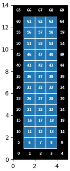
Figure 2.
Model but with designated cell numbers.
3.1.1. Assumptions
The scenario in [18,19] states that there are 68 passengers total on the bus, including the driver, and that there are 15 rows of seats. It is unclear exactly what type of bus was used for travel; however, if we use data from [35], we have that a reasonable estimate is 12.1 m in length, 2.58 m in width, and 2.95 m in height. For our purposes, as we need there to be nonfractional units, we assume the bus is 12 m by 3 m by 3 m.
The bus contained four windows that could be opened; however, for ease of computation, we assume they stay shut for the duration of the ride. It is also known that the bus had warm air vents every two rows that were the outlets for air to be circulated back into the bus. It is not stated where the air inlet on this bus was, but again, from [35], we can make an assumption that it was located on the back panel of the bus. We also let the bus ride be one 100 min ride, so no agents move.
As we must keep all cells in one meter by one meter sizes, we have to do our best to give the proper placings of people and outlet vents. On the left side of the bus, we allow the driver to be in , and then no one is in ; and then we average out the number of people (40 total), so we have about four people per meter. On the right side (28 total), we average out roughly 3 people per meter, with a few distinctions (such as the middle seat in which there was no passenger) to have 2 people.
We positioned 14 outlets, 7 on each side, every 2 rows starting from the bottom of the bus, with an extra set in the row starting at , as we tried to space them as evenly as possible while still having outlets in the front row and back row. The air inlet is positioned at to coincide with being on the back panel. This gives us roughly a similar layout to the bus shown in [18].
Due to the fact that SARS-CoV-2 rarely produces sneezing [36], we assume that our infector does not sneeze at all. Due to being among mostly other elderly temple worshipers, and because we have no idea of the closeness of those riding the bus, we assume that no one talks either. As coughing can happen at any time, to anyone, and it is easy to cough several times in a chain, we have on average that our infector coughs ten times over the course of the trip. We also assume that the infector is always looking forward, as one would typically do on a bus; thus, all viral material is spread towards the direction of the front of the bus.
3.1.2. Sensitivity Analysis for Ventilation Effects
Before we begin our actual test, we want to obtain a better understanding of how differing levels of filtration and numbers of air changes per hour affect the number of infections overall. To understand how filtration rates affect infection rates, we hold the ventilation rate (ACH) constant and vary filtration rates. We used 60 ACH for every trial; this is consistent with what we believe a bus would typically have for ventilation rate [35], and we varied the filtration rate between 0% and 40%. To see how ventilation rates affect infection rates, we hold the filtration rate constant at 20%, which is again what we typically believe a bus such as this has [35], and vary the ventilation rate from 2 to 60 ACH. We do not start at 0, only because our model relies on movement, and with only 100 min for the bus rides, values of less than 2 do not capture enough frames to make use of the ventilation system; thus, the results are not valid.
Our results in Figure 3a indicate that with a ventilation rate of 60 ACH, we see a large degradation in the number of infections present as we increase filtration rate. Our model indicates that if there were no filtration present at all, nearly all of the riders would have most likely been infected. However, this is not quite a realistic scenario, as even with no filter, there is a relatively low chance that no virions would be caught in the front or sides of the inlet or ventilation tubing. This finding also indicates that at a high ACH value, going from a 0% filtration rate to a 10% filtration rate would cut down roughly half of all infections, and thus, for small highly ventilated spaces, any filter would be highly effective at stopping virion transfer.

Figure 3.
Infections against varying ventilation and filtration rate: (a) Varying filtration, 60 ACH, 1000 runs per filtration rate, average 10 coughs, 0 sneezing, and 0 talking. (b) Varying ACH, 20% filtration rate, 1000 runs per ACH, average 10 coughs, 0 sneezing, and 0 talking.
Our results in Figure 3b indicate that with a filtration rate of 20%, we see a large degradation in the number of infections present as we increase the ventilation rate. Our model indicates that very low ventilation rates (<5 ACH) would see roughly 90% of riders become infected, and roughly for every 10 ACH added, we drop infection rates by about 10%.
One thing to notice about these figures is that increasing the ventilation rate decreased the infection rate in almost a linear fashion. However, this is not the case with varying the filtration rate. Varying the filtration rate was quite a bit more effective at the lower rates, only requiring a change from capturing 0% to capturing 10% to reduce infection from roughly 100% to roughly 55%. However, when the filtration rate is changed from 10 to 20%, the infection rate is reduced from roughly 50% to roughly 35%.
3.1.3. Sensitivity Analysis for Spread Vectors
In this section, we look to find out how different vectors of infection impact the infection rates overall on the bus. Below, we consider differing numbers of sneezes, coughs, and minutes talked and compare and contrast them. All trials will be conducted with the index infector sitting at (more on this reasoning in the next section), with the ventilation inlet at . We once again assume that 20% of air is filtered and that there is 60 ACH. For each vector of infection, we set the other nonbreathing infection vectors to 0, so that we can best isolate the effects of the singular method we are observing. This means if we are looking at minutes talked, for example, then breathing continues as normal, but there is no sneezing and no coughing from the index infector.
Going back to the original values of virions spread for our four vectors, they were all one order of magnitude above each other: talking spread an order of magnitude more virions than breathing, coughing an order of magnitude more than talking, and sneezing an order of magnitude over coughing, alongside the distances the virions traveled. If our model only cared about the number of virions in the system, then we should see that the infection rate for 10 min of talking should be the same for one cough and continue growing linearly from there.
However, considering our findings in Figure 4, while that is true for small amounts such as 10 min of talking to 1 cough, it becomes less true as the numbers get larger. Specifically, comparing talking to coughing, when the infector talks the entire bus ride, the infections are roughly 25%, but if we allow the person to cough 10 times, we attain an infection percentage of roughly 40%. When comparing the graphs for coughing and sneezing, we no longer even attain roughly the same numbers at small values. When the infector has coughed 10 times, equivalent in magnitude to sneezing 1 time, the infection rate for the single sneeze is almost 60%. When we look at 2 sneezes versus 20 coughs, the difference becomes even more stark, with the 2 sneezes infecting roughly 80% of the bus, while the 20 coughs only infect roughly 65% of the bus.
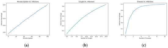
Figure 4.
Infections against varying ACH or filtration rate: (a) 1000 runs per number of minutes talked on average; (b) 1000 runs per number of coughs on average; and (c) 1000 runs per number of sneezes on average.
By inspecting the shapes of the graphs, we can see there is a trend. When there are more virions spread at a single time, versus spread out over time, the infections over time increase sharply. This leads us to believe that our model indicates ventilation over time deals with smaller amounts of particles better than trying to deal with large amounts at the same time.
3.1.4. Testing Best Guess
We now attempt to get as close to the real scenario as possible. As the index infector was seated in row 8, corresponding to our model, this would be roughly or . We chose to put the index infector in arbitrarily, and there was not much difference in infection rates or spread of infection between the two. We assume that 20% of air is filtered each time through the system [35]. Below, we detail our attempt at the main scenario, as well as how moving the index infector to different parts of the bus would affect infection rates in our model. The red cell in all bus figures indicates the position of the index infector.
Our results in Figure 5 indicate that there is a 41.9% infection rate (including the index infector) throughout the bus overall. By removing the index infector, we obtain an infection rate of 41%, which is well within the 95% confidence interval of 24.1 to 46.3%, with an attack rate of 34.3% during the actual bus ride.

Figure 5.
1000 runs, 60 ACH, 20% Filtration, Infector at , and 41.9% Infected.
We can see that by inspecting Table A1, the overall infection rate 95% confidence interval is (0.415, 0.423), and that all of the 95% confidence intervals for each cell are within a similarly tight range. Thus, we can be confident that 1000 runs is enough for us to obtain accurate data from our model, and we can use that number for the rest of the tests to come.
The main difference between our model and the actual infections is in where the infections took place. Inspecting Figure 5 shows us that a large proportion of the infections took place towards the inlet at the back of the bus. On average, in our model, 11.88 infections took place directly behind the index infector towards the inlet, and the likelihood of infection was slightly higher the further back we look in the bus. However, in the real scenario, only seven of the infections took place in these areas, and there is a clear indication that the number of infected does not rise as we go towards the back of the bus but stays larger in more local rows to the index infector.
There are two possible reasons that we can think of that may lead to this outcome. The first possibility stems from not knowing where the air inlet is located, and as our model is made to pull virions towards the inlet, virions would be pulled backwards from the index infector over the seats behind. In our model, we created a sort of virion loop towards the back that constantly bathes the agents seated next to the inlet with virions being passed over them both from the virions directly in front from the index infector and the outlet pushing virions back over them.
The second possibility is that in the real scenario, two of the four windows that could be opened were at the very back of the bus in the final two rows. We assumed that these would be shut for our model; however, there is no mention in [18,19] of whether or not these were opened during the trip. If these windows were to be opened, it would lead to the back of the bus being flush with fresh air; thus, those nearest these windows may not have been affected as they would have been if the windows were shut.
3.1.5. Differing Placement of Index Infector
Now, we would like to see how placing the index infector in different positions would change the results of our test. Our theoretical placements here occur on the right side of the bus, in for the back, for the middle directly across from the actual index infector’s seat, and for the front.
In Figure 6b, we see similar results to our actual test case, having an average of 41.2% of those onboard ending up infected with a 95% confidence interval of (0.408, 0.416). Our model indicates that there will still be a larger amount of infections towards the back of the bus, where the inlet is; the distribution and number of infected overall are both like their counterparts in the main index infector position.
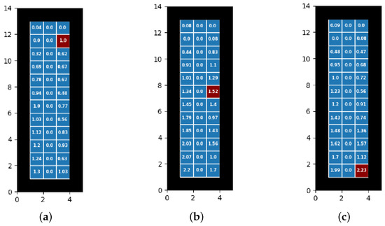
Figure 6.
Infection rates and distributions for differing placement on right side of bus: (a) Front right (), 26.2% infected. (b) Middle right (), 41.2% infected. (c) Back right (), 34.7% infected.
In Figure 6a, the main thing to notice from this position is that the number of infections overall is lower, at 26.2% (95% CI of (0.259, 0.266)) versus the 41.2% of the middle index infector position. We once again notice a general gradient of infections the further back in the bus the agents are located. As before, it is likely that cells near an inlet and an outlet create a virion loop that constantly funnels virions into these cells.
In Figure 6c, we have an average overall proportion of infections as 34.7% (95% CI (0.344, 0.351)). One interesting thing to note about this placement is that the infection rate is quite a bit higher (34.7% vs. 26.2%) when placing the index infector in the back versus placing it in the front, but it is not as high as when it is placed in the middle (34.7% vs. 41.2%). This gives us an indication that both the ventilation system and spreading of virions directly from the index infector combine to infect the most people. Once again, we see that the back four cells had by far the highest concentration of infections, another indication that the virions loops we previously stated are stronger the closer the index infector is to the inlet.
As we saw previously in the original trial, the 95% confidence intervals are once again quite tight for all positions on the bus over 1000 runs.
4. Discussion and Conclusions
We believe that our model validates the use of a simple stochastic movement ABM for dealing with aerosol-based infectious diseases. It is not the goal of this manuscript to dethrone the use of computational fluid dynamics ABM’s but to give a simple alternative with far lesser hardware requirements to run. We saw relatively similar results when speaking of overall infections on the bus versus what happened in real life. Our average numbers of infections were well within the stated 95% confidence interval of the original study that we reference. We hope that in the future, others will be able to modify assumptions and methods of a simple stochastic model to achieve an even more realistic model. However, even with this model, we are still able to make some conclusions.
Our model indicates several key factors to us that are important in understanding what may have happened on the bus in Ningbo and give insights into where those who have infectious diseases that are primarily distributed by aerosols should be placed if there is no other option than to be in a tight space with some sort of ventilation.
First, when comparing filtration rates and ventilation rates, we notice that the most important thing to do is get some type of filtration. When we increased the filtration rate above 0%, we saw the sharpest decline in infections of any other test.
Secondly, our model indicates that spreading smaller amounts of virions through acts such as breathing and light talking, but in a more consistent manner, is less effective at infecting other people in the vicinity as opposed to spreading large numbers of virions at once through acts such as sneezing and coughing.
Finally, we understand that placing infectious people away from inlets in a closed ventilation system does help a bit in stopping more viral material from spreading throughout space, but it is even more effective to place the infected person away from most of the other people in the space and to try and have them not spread virions directly onto others. On the real-life bus, our model indicates the index infector was just about in the worst possible spot with regard to infecting others.
One interesting thing that our model made us realize is that placing inlets and outlets right next to each other is most likely not a good idea; in real life, there may even be more settling inside the system than we accounted for, but even without that, there seems be a tunnel of viral material created that is constantly bathing the people in the middle of these loops, in which they would become more infected, more often. This did not seem to be the case when looking at the real-life infections in [18], but as stated before, there are other possible reasons that this may not have happened.
We believe this has all shown that simple stochastic agent models are worth investigating further with regard to aerosol-based diseases. Our model can be easily adapted by changing certain parameters for known diseases such as SARS, MERS, the flu, and others by changing the infection parameters found in the construction section. As these types of diseases are also highly infectious through aerosols, they share many of the same terminologies as SARS-CoV-2. With these types of illnesses, people will still be able to spread them through breathing, talking, coughing, and sneezing. This lends itself to being able to regard these other illnesses while only changing the number of virions in saliva and an estimate of the number of virions needed to infect a susceptible agent with one of these illnesses. We also believe that even with this basic sort of model, we gained some valuable insight into the placement of infectors and the concentration of aerosol spread vectors on infection rates.
Finally, we believe that this type of model has the possibility of being used by companies and services that require many people to be stuck in an enclosed space. If an emerging illness is being spread, time is short to put together a reasonable estimate of safety precautions. A model that is less computationally expensive, with fewer necessary parameters, would be reasonable for creating a risk factor analysis for those that may utilize their service. The service itself might also be able to better understand the impacts of a new disease on their service quickly and allow for more flexibility when creating plans to combat the new illness.
Limitations
Our model is of course not without shortcomings. Some further research for this experiment is to see how smaller ventilation rates correspond with differing filtration rates as well; unfortunately, due to computational power restraints, this would have taken an exorbitant amount of time to complete for us using the hardware we are attempting the simulations on.
Of course, as has already been touched upon, the validation scenario is our best guess as to what the real situation was like. However, with the difficulty of obtaining comprehensive real-life data (as one would need to be actively testing at the time of infections and note everything possible), we feel the used scenario was as close as possible to comprehensive for the purpose of our trials. We do note however that we have chosen to allow infections to be calculated at the end of the study. If this model were to be adapted to a longer time period, there would necessarily be additions regarding other agents becoming infectors in the middle of the simulation. However, this means it is still not complete and thus must be included as a limitation in our trial.
Other limitations with regard to data control are things such as humidity and temperature, vaccine status, immunodeficiency, age, and a plethora of other such factors. Each of these types of variations can have an effect on the outcome of the experiment, and it would be encouraged to look into findings that have these parameters added. However, in this experiment, we did not have any reasonable data to look to and add to our simulation, and they were thus not added as parameters.
We also tested what would happen if we placed the inlet more towards the front middle of the bus, where it would not be placed in a wall. The results are promising with regard to infection rates and distribution; however, because of the way that our model designates the shortest path to inlets, a problem arose with the number of infections directly next to the inlet, and thus, these results are omitted. Further work in the future may be carried out to correctly mitigate this issue.
In general, there are various scenarios that are different from our own, such as those in other enclosed ventilated spaces. These spaces could be within airplanes, trains, subways, meeting rooms, cafeterias, or many others. All of these types of scenarios may have one or more infectors and may be considered with differing timespans of superspreading events. In this manuscript, we are specifically looking at how one infected superspreader over a short period of time can infect others in these enclosed spaces, but it is absolutely possible to also consider having more than one infector, or having the agents move about the space if the scenario allows, which could be tested using the approach we created. Recall that in our model, the probability of a susceptible agent developing the disease once exposed to the virus is calculated using Equation (1) of Section 2.2. As such, in all these varied scenarios, the important adjustment will be how to determine the volume (V) of the saliva (as elaborated in Appendix B) that a susceptible agent is exposed to. There are also many different variations of the model we created that could use similar ideas to create quick stochastic movement paradigms for virion spread.
This study is by no means comprehensive, as one of the main goals of this manuscript was to give a validation of the implementation of a simple model such as this for future endeavors. We believe, however, that there is enough evidence for an approach such as this using simple low-power agent modeling for more investigation with regard to aerosol-based disease spread in small spaces with ventilation.
Author Contributions
M.G.: conceptualization, data curation, formal analysis, investigation, methodology, software, visualization, writing—original draft, and writing—review and editing; V.M.: conceptualization, supervision, methodology, and writing—review and editing; J.S.: conceptualization, methodology, software, and writing—review and editing. All authors have read and agreed to the published version of the manuscript.
Funding
This research received no external funding.
Institutional Review Board Statement
Not applicable.
Informed Consent Statement
Not applicable.
Data Availability Statement
Not applicable.
Acknowledgments
We would like to thank the Pharr Fellowship from Washington State University for their monetary contribution to this work.
Conflicts of Interest
The authors declare no conflict of interest.
Appendix A. Statistical Tables for Differing Placement of Infector

Table A1.
Infector at .
Table A1.
Infector at .
| Cell | Mean | 95% CI Left Bound | 95% CI Right Bound |
|---|---|---|---|
| 6 | 1.988 | 1.926 | 2.050 |
| 8 | 2.231 | 2.188 | 2.274 |
| 11 | 1.703 | 1.641 | 1.765 |
| 13 | 1.115 | 1.071 | 1.159 |
| 16 | 1.619 | 1.557 | 1.681 |
| 18 | 1.567 | 1.511 | 1.623 |
| 21 | 1.484 | 1.424 | 1.544 |
| 23 | 1.357 | 1.302 | 1.412 |
| 26 | 1.434 | 1.374 | 1.494 |
| 28 | 0.735 | 0.692 | 0.778 |
| 31 | 1.2 | 1.144 | 1.256 |
| 33 | 0.908 | 0.859 | 0.957 |
| 36 | 1.229 | 1.172 | 1.286 |
| 38 | 0.557 | 0.518 | 0.596 |
| 41 | 1.002 | 0.948 | 1.056 |
| 43 | 0.721 | 0.675 | 0.767 |
| 46 | 0.954 | 0.900 | 1.008 |
| 48 | 0.683 | 0.638 | 0.728 |
| 51 | 0.477 | 0.438 | 0.516 |
| 53 | 0.467 | 0.427 | 0.507 |
| 58 | 0.084 | 0.067 | 0.101 |
| 61 | 0.087 | 0.070 | 0.104 |
| Overall | 0.347 | 0.344 | 0.351 |
Table A2.
Infector at .
Table A2.
Infector at .
| Cell | Mean | 95% CI Left Bound | 95% CI Right Bound |
|---|---|---|---|
| 6 | 2.229 | 2.168 | 2.290 |
| 8 | 1.595 | 1.541 | 1.649 |
| 11 | 2.024 | 1.962 | 2.086 |
| 13 | 1.011 | 0.967 | 1.055 |
| 16 | 2.083 | 2.021 | 2.145 |
| 18 | 1.518 | 1.464 | 1.572 |
| 21 | 1.861 | 1.797 | 1.925 |
| 23 | 1.342 | 1.286 | 1.398 |
| 26 | 1.925 | 1.864 | 1.986 |
| 28 | 0.848 | 0.804 | 0.892 |
| 31 | 1.773 | 1.711 | 1.835 |
| 33 | 1.115 | 1.062 | 1.168 |
| 36 | 2.511 | 2.458 | 2.564 |
| 38 | 0.655 | 0.613 | 0.697 |
| 41 | 1.652 | 1.591 | 1.713 |
| 43 | 0.755 | 0.710 | 0.800 |
| 46 | 1.457 | 1.397 | 1.517 |
| 48 | 0.721 | 0.674 | 0.768 |
| 51 | 0.791 | 0.743 | 0.839 |
| 53 | 0.492 | 0.453 | 0.531 |
| 58 | 0.081 | 0.064 | 0.098 |
| 61 | 0.07 | 0.054 | 0.086 |
| Overall | 0.419 | 0.415 | 0.423 |
Table A3.
Infector at .
Table A3.
Infector at .
| Cell | Mean | 95% CI Left Bound | 95% CI Right Bound |
|---|---|---|---|
| 6 | 2.196 | 2.133 | 2.259 |
| 8 | 1.696 | 1.642 | 1.750 |
| 11 | 2.067 | 2.006 | 2.128 |
| 13 | 0.998 | 0.954 | 1.042 |
| 16 | 2.027 | 1.965 | 2.089 |
| 18 | 1.559 | 1.505 | 1.613 |
| 21 | 1.852 | 1.789 | 1.915 |
| 23 | 1.432 | 1.378 | 1.486 |
| 26 | 1.788 | 1.726 | 1.850 |
| 28 | 0.968 | 0.923 | 1.013 |
| 31 | 1.453 | 1.394 | 1.512 |
| 33 | 1.396 | 1.341 | 1.451 |
| 36 | 1.342 | 1.283 | 1.401 |
| 38 | 1.522 | 1.491 | 1.553 |
| 41 | 1.008 | 0.954 | 1.062 |
| 43 | 1.29 | 1.237 | 1.343 |
| 46 | 0.907 | 0.854 | 0.960 |
| 48 | 1.098 | 1.046 | 1.150 |
| 51 | 0.441 | 0.404 | 0.478 |
| 53 | 0.831 | 0.782 | 0.880 |
| 58 | 0.076 | 0.060 | 0.092 |
| 61 | 0.081 | 0.064 | 0.098 |
| Overall | 0.412 | 0.408 | 0.416 |
Table A4.
Infector at .
Table A4.
Infector at .
| Cell | Mean | 95% CI Left Bound | 95% CI Right Bound |
|---|---|---|---|
| 6 | 1.3 | 1.242 | 1.358 |
| 8 | 1.026 | 0.975 | 1.077 |
| 11 | 1.244 | 1.188 | 1.300 |
| 13 | 0.631 | 0.590 | 0.672 |
| 16 | 1.205 | 1.148 | 1.262 |
| 18 | 0.926 | 0.876 | 0.976 |
| 21 | 1.117 | 1.060 | 1.174 |
| 23 | 0.831 | 0.781 | 0.881 |
| 26 | 1.029 | 0.976 | 1.082 |
| 28 | 0.561 | 0.522 | 0.600 |
| 31 | 0.998 | 0.942 | 1.054 |
| 33 | 0.772 | 0.724 | 0.820 |
| 36 | 0.936 | 0.884 | 0.988 |
| 38 | 0.484 | 0.446 | 0.522 |
| 41 | 0.778 | 0.729 | 0.827 |
| 43 | 0.666 | 0.620 | 0.712 |
| 46 | 0.694 | 0.648 | 0.740 |
| 48 | 0.671 | 0.625 | 0.717 |
| 51 | 0.318 | 0.284 | 0.352 |
| 53 | 0.62 | 0.577 | 0.663 |
| 61 | 0.041 | 0.029 | 0.053 |
| Overall | 0.262 | 0.259 | 0.266 |
Appendix B. Expanded Model Construction
Appendix B.1. Cell Population
As stated, each cell contains a list of its population every frame. When we display the number of agents in a cell, we use a varying shade of red. The darker the red, the more population is in the cell. An example of what this may look like can be found in Figure A1 below.

Figure A1.
Population visualization (black denotes inaccessible cells, such as walls).
Depending on the circumstance of the scenario being modeled, adjustments can be made for when and how the agents check their infection status. In the circumstance to be discussed in Section 3 we have each member of the population check its infection status at the end.
Appendix B.2. Cell Virions
We can visualize the number of virions in a cell by denoting the density of virions with a shade of blue, an example of what one such frame may look like is in Figure A2 below.

Figure A2.
Virion visualization and movement: (a) Sample virions with colors, black denotes inaccessible cells (such as walls). (b) Virion movement within a Moore neighborhood.
Distribution of Virions
To make calculations simple, we assume that each vector of virion spread works in the same way, except for different distances, with different distributions per cell. We assume that virions that are spread to other cells are completely mixed within the entire air volume of said cell. We define the air volume of a cell as the air contained in the 2D plane and extended up to the ceiling. For example, a 5 m ceiling gives us 5 m3 of air volume, since we assume each cell is 1 m by 1 m.
Appendix B.3. Ventilation Cells
Ventilation is a central part of our model, and it is how we determine how many frames a single run of the model uses.
Appendix B.3.1. Inlet Cells
Our ventilation system works by using inlets and outlets to transfer virions throughout the environment. To facilitate the movement of virions in a scenario, we assume that each frame virions move towards the closest air inlet to them. For example, consider the scenario below:
 where contains the virions we are considering, and the inlet vents are located at the bottom left corner and the top right corner . In this scenario, virions travel towards , as it is the closer inlet, and the virions randomly pick a path that moves them towards that vent at every frame to take into account any sort of crosswind patterns.
Figure A3.
Movement of virions towards inlet cell .
To obtain this random path, the current cell understands which adjacent cells are closer to the inlet than itself, and if there is more than one possible option, virions have an equal probability of moving to any of the closer adjacent cells. In the scenario above, the closer adjacent cells are highlighted in red, as each of the red cells are only one cell away from ; thus, the entire mass of virions moves to either or with equal probability.
As stated in Appendix B.2, this movement of virions towards the inlet cells is what constitutes in the total virions of a cell.
Figure A2b shows the possible destinations for a particular cell’s virions centered in the middle cell within a Moore neighborhood, a typical eight-way directional movement scheme.
Each infected agent in a cell creates a new set of virions based on what vector of transportation is being used between breathing, talking, coughing, and sneezing. The number of virions produced by these vectors is given by , , , and , respectively. corresponds to the movement of virions that are already existing in the space given by crosswind patterns each frame, and is given by the number of virions placed back into circulation by the ventilation outlets (more on these in Appendix B.3.1 and Appendix B.3.2). Using the values from [20], we calculate the number of virions in a cell as
Appendix B.3.2. Outlet Cells
Outlet cells, like inlet cells, are placed in a cell and act as return systems for the previously filtered virions. Each outlet has a face direction that is set before each simulation, when the outlet cells are designated. This face direction is the direction that outlets will move their virions in. Consider the following scenario, where the outlet cell is located at and is highlighted green, with face direction to the left.

Figure A4.
Movement of virions out of cell .
Each outlet moves virions 2 m outward in the direction that it is aimed; in the scenario above, the virions would be equally distributed to the three cells that are highlighted in blue. If the outlet cell is designated as a wall, then only two cells outward have virions, and both of them receive an equal share.
If, for instance, there were outlets located at and with face directions of left, right, left, respectively, we obtain a scenario that looks like before the virions once again start moving towards the nearest inlet in the next frame. The virions in each of these cells given by the outlets are what constitutes from Appendix B.2.

Figure A5.
Multiple outlet cells releasing virions.
Appendix B.3.3. Spreading Virions through Breathing
Every frame, our infected agents breathe out a number of virions. As stated before, this is at a rate of , with being the rate at which an average person exhales air per minute [20]. Since breathing virions does not extend beyond the initial cell in our model, 100% of the virions distributed outward are contained within the initial cell and mixed instantaneously with the air contained in the cell.
Appendix B.3.4. Spreading Virions through Talking
Each frame has a probability that our agent will talk, thus spreading virions in a different manner than just breathing. There is evidence that the volume of talking changes the expulsion force and virion contribution to the surrounding air [37,38,39]. However, since in most cases it is difficult to know the actual volume of talking to better understand expulsion, we default back to the values from [20].
As stated before, the rate of virion spread through talking is given by , with being the average rate a person expels virions through aerosols in [20]. Since we assumed talking to have virions travel 1 m forward, we have that all virions will be only in the short-range category, and for ease of computation, we assume that virions are evenly spread among their distance category; this means that in this scenario with short-range aerosols, half of the virions are within the main cell, and half are one cell away. We assume that the air volume in each cell instantly mixes with the virions.
Appendix B.3.5. Spreading Virions through Coughing and Sneezing
Each frame has a probability that our agent will cough or sneeze; we have that coughing is common among SARS-CoV-2 patients, while sneezing is rare [36]. Similarly to talking, it is hard to quantify how often an agent would cough, or what the cough probability will be. We consider this probability more directly in the given scenarios.
We assume that a cough includes the immediate cell and three cells forward; thus, two cells consist of short-range aerosols and two cells consist of long-range aerosols. As before, we assume that half of the short-range aerosols reside in each of the closest two cells, and half of the long-range aerosols reside in the further two cells.
As we are purely looking at short- and long-range aerosols, we have that short-range make up 80.8% of the virions, while long-range make up 19.2% of the virions when coughing. For sneezing, we follow the same style of spread as previously, where each class of aerosols has its virions equally spread between the cells it will infect, and for sneezing, we have that 70.2% of virions are short-range aerosols, 16.7% of virions reside in long-range aerosols, and 13.1% of virions reside in buoyant aerosols [24]. For both the sneezing and coughing vectors of spread, we also assume that once virions enter the cells, they are instantly mixed with the air of that cell.
For coughing, the rate of virions spread is given by , and sneezing is given by [20].
References
- Jones, R.M. Aerosol transmission of infectious disease. Occup. Environ. Med. 2015, 5, 501–508. [Google Scholar] [CrossRef] [PubMed]
- WHO Coronavirus (COVID-19) Dashboard. 2023. Available online: https://covid19.who.int/ (accessed on 25 April 2023).
- Chia, P.Y.; Coleman, K.K.; Tan, Y.K.; Ong, S.W.X.; Gum, M.; Lau, S.K.; Lim, X.F.; Lim, A.S.; Sutjipto, S.; Lee, P.H.; et al. Detection of air and surface contamination by SARS-CoV-2 in hospital rooms of infected patients. Nat. Commun. 2020, 11, 2800. [Google Scholar] [CrossRef] [PubMed]
- Mondelli, M.U.; Colaneri, M.; Seminari, E.M.; Baldanti, F.; Bruno, R. Low risk of SARS-CoV-2 transmission by fomites in real-life conditions. Lancet Infect. Dis. 2021, 21, e112. [Google Scholar] [CrossRef] [PubMed]
- Cheng, P.; Luo, K.; Xiao, S.; Yang, H.; Hang, J.; Ou, C.; Cowling, B.J.; Yen, H.L.; Hui, D.S.C.; Hu, S.; et al. Predominant airborne transmission and insignificant fomite transmission of SARS-CoV-2 in a two-bus COVID-19 outbreak originating from the same pre-symptomatic index case. J. Hazard. Mater. 2022, 425, 128051. [Google Scholar] [CrossRef]
- Liu, H.; He, S.; Shen, L.; Hong, J. Simulation-based study of COVID-19 outbreak associated with air-conditioning in a restaurant. Phys. Fluids 2021, 33, 023301. [Google Scholar] [CrossRef]
- Bertozzi, A.L.; Franco, E.; Mohler, G.; Short, M.B.; Sledge, D. The challenges of modeling and forecasting the spread of COVID-19. Proc. Natl. Acad. Sci. USA 2020, 117, 16732–16738. [Google Scholar] [CrossRef]
- Tovissodé, C.F.; Lokonon, B.E.; Kakaï, R.G. On the use of growth models to understand epidemic outbreaks with application to COVID-19 data. PLoS ONE 2020, 15, e0240578. [Google Scholar] [CrossRef]
- Motamedi, H.; Shirzadi, M.; Tominaga, Y.; Mirzaei, P.A. CFD modeling of airborne pathogen transmission of COVID-19 in confined spaces under different ventilation strategies. Sustain. Cities Soc. 2022, 76, 103397. [Google Scholar] [CrossRef]
- Hussein, T.; Löndahl, J.; Thuresson, S.; Alsved, M.; Al-Hunaiti, A.; Saksela, K.; Aqel, H.; Junninen, H.; Mahura, A.; Kulmala, M. Indoor Model Simulation for COVID-19 Transport and Exposure. Int. J. Environ. Res. Public Health 2021, 18, 2927. [Google Scholar] [CrossRef]
- Yanev, N.M.; Stoimenova, V.K.; Atanasov, D.V. Branching stochastic processes as models of COVID-19 epidemic development. arXiv 2020, arXiv:2004.14838. [Google Scholar]
- Cooper, I.; Mondal, A.; Antonopoulos, C.G. A SIR model assumption for the spread of COVID-19 in different communities. Chaos Solitons Fractals 2020, 139, 110057. [Google Scholar] [CrossRef] [PubMed]
- Ud Din, R.; Algehyne, E.A. Mathematical analysis of COVID-19 by using SIR model with convex incidence rate. Results Phys. 2021, 23, 103970. [Google Scholar] [CrossRef]
- Mariam; Magar, A.; Joshi, M.; Rajagopal, P.S.; Khan, A.; Rao, M.M.; Sapra, B.K. CFD Simulation of the Airborne Transmission of COVID-19 Vectors Emitted during Respiratory Mechanisms: Revisiting the Concept of Safe Distance. ACS Omega 2021, 6, 16876–16889. [Google Scholar] [CrossRef]
- Sarhan, A.R.; Naser, P.; Naser, J. COVID-19 aerodynamic evaluation of social distancing in indoor environments, a numerical study. J. Environ. Health Sci. Eng. 2021, 19, 1969–1978. [Google Scholar] [CrossRef]
- Ren, C.; Xi, C.; Wang, J.; Feng, Z.; Nasiri, F.; Cao, S.J.; Haghighat, F. Mitigating COVID-19 infection disease transmission in indoor environment using physical barriers. Sustain. Cities Soc. 2021, 74, 103175. [Google Scholar] [CrossRef]
- Gaddis, M.D.; Manoranjan, V.S. Modeling the Spread of COVID-19 in Enclosed Spaces. Math. Comput. Appl. 2021, 26, 79. [Google Scholar] [CrossRef]
- Shen, Y.; Li, C.; Dong, H.; Wang, Z.; Martinez, L.; Sun, Z.; Handel, A.; Chen, Z.; Chen, E.; Ebell, M.H.; et al. Community Outbreak Investigation of SARS-CoV-2 Transmission among Bus Riders in Eastern China. JAMA Intern. Med. 2020, 180, 1665–1671. [Google Scholar] [CrossRef] [PubMed]
- Lin, J.; Yan, K.; Zhang, J.; Cai, T.; Zheng, J. A super-spreader of COVID-19 in Ningbo city in China. J. Infect. Public Health 2020, 13, 935–937. [Google Scholar] [CrossRef]
- Evans, M.J. Avoiding COVID-19: Aerosol Guidelines. medRxiv 2020. [Google Scholar] [CrossRef]
- Syder, W.S.; Cook, M.J.; Nasset, E.S.; Karhausen, L.R.; Howells, G.P.; Tipton, I.H. Report on the Task Group of Reference Men; International Commission on Radiological Protection: London, UK, 1974. [Google Scholar]
- Wells, W.F. On air-borne infectionstudy II. droplets and droplet nuclei. Am. J. Epidemiol. 1934, 20, 611–618. [Google Scholar] [CrossRef]
- Watanabe, T.; Bartrand, T.A.; Weir, M.H.; Omura, T.; Haas, C.N. Development of a Dose-Response Model for SARS Coronavirus. Risk Anal. 2010, 30, 1129–1138. [Google Scholar] [CrossRef] [PubMed]
- Chen, P.Z.; Bobrovitz, N.; Premji, Z.; Koopmans, M.; Fisman, D.N.; Gu, F.X. Heterogeneity in transmissibility and shedding SARS-CoV-2 via droplets and aerosols. eLife 2021, 10, e65774. [Google Scholar] [CrossRef] [PubMed]
- Xie, X.; Li, Y.; Chwang, A.T.Y.; Ho, P.L.; Seto, W.H. How far droplets can move in indoor environments—Revisiting the Wells evaporation–falling curve. Indoor Air 2007, 17, 211–225. [Google Scholar] [CrossRef] [PubMed]
- Tellier, R. Aerosol transmission of influenza A virus: A review of new studies. J. R. Soc. Interface 2009, 6, S783–S790. [Google Scholar] [CrossRef] [PubMed]
- Kutter, J.S.; Spronken, M.I.; Fraaij, P.L.; Fouchier, R.A.M.; Herfst, S. Transmission routes of respiratory viruses among humans. Curr. Opin. Virol. 2018, 28, 142–151. [Google Scholar] [CrossRef]
- Teunis, P.F.M.; Brienen, N.; Kretzschmar, M.E.E. High infectivity and pathogenicity of influenza A virus via aerosol and droplet transmission. Epidemics 2010, 2, 215–222. [Google Scholar] [CrossRef] [PubMed]
- Dhand, R.; Li, J. Coughs and Sneezes: Their Role in Transmission of Respiratory Viral Infections, Including SARS-CoV-2. Am. J. Respir. Crit. Care Med. 2020, 202, 651–659. [Google Scholar] [CrossRef]
- El Hassan, M.; Assoum, H.; Bukharin, N.; Al Otaibi, H.; Mofijur, M.; Sakout, A. A review on the transmission of COVID-19 based on cough/sneeze/breath flows. Eur. Phys. J. Plus 2021, 137, 1–36. [Google Scholar] [CrossRef]
- Mousavi, E.; Pollitt, K.; Sherman, J.; Martinello, R. Performance analysis of portable HEPA filters and temporary plastic anterooms on the spread of surrogate coronavirus. Build. Environ. 2020, 183, 107186. [Google Scholar] [CrossRef]
- ASHRAE. ASHRAE Position Document on Infectious Aerosols; ASHRAE: Peachtree Corners, GA, USA, 2022. [Google Scholar]
- EPA. What Is a MERV Rating? EPA: Washington, DC, USA, 2022. [Google Scholar]
- EPA. How Much Ventilation Do I Need in My Home to Improve Indoor Air Quality? EPA: Washington, DC, USA, 2022. [Google Scholar]
- Zhang, Z.; Han, T.; Yoo, K.H.; Capecelatro, J.; Boehman, A.L.; Maki, K. Disease transmission through expiratory aerosols on an urban bus. Phys. Fluids 2021, 33, 015116. [Google Scholar] [CrossRef]
- COVID-19, Cold, Allergies and the Flu: What Are the Differences? 2021. Available online: https://www.mayoclinic.org/diseases-conditions/coronavirus/in-depth/covid-19-cold-flu-and-allergies-differences/art-20503981 (accessed on 4 September 2022).
- Asadi, S.; Wexler, A.S.; Cappa, C.D.; Barreda, S.; Bouvier, N.M.; Ristenpart, W.D. Aerosol emission and superemission during human speech increase with voice loudness. Sci. Rep. 2019, 9, 2348. [Google Scholar] [CrossRef] [PubMed]
- Binazzi, B.; Lanini, B.; Bianchi, R.; Romagnoli, I.; Nerini, M.; Gigliotti, F.; Duranti, R.; Milic-Emili, J.; Scano, G. Breathing pattern and kinematics in normal subjects during speech, singing and loud whispering. Acta Physiol. 2006, 186, 233–246. [Google Scholar] [CrossRef] [PubMed]
- Bake, B.; Larsson, P.; Ljungkvist, G.; Ljungström, E.; Olin, A.C. Exhaled particles and small airways. Respir. Res. 2019, 20, 8. [Google Scholar] [CrossRef] [PubMed]
Disclaimer/Publisher’s Note: The statements, opinions and data contained in all publications are solely those of the individual author(s) and contributor(s) and not of MDPI and/or the editor(s). MDPI and/or the editor(s) disclaim responsibility for any injury to people or property resulting from any ideas, methods, instructions or products referred to in the content. |
© 2023 by the authors. Licensee MDPI, Basel, Switzerland. This article is an open access article distributed under the terms and conditions of the Creative Commons Attribution (CC BY) license (https://creativecommons.org/licenses/by/4.0/).