1. Introduction
The world is experiencing for the first time in its history a multidimensional crisis at a global level, caused by the severe acute respiratory syndrome COVID-19 (SARS-CoV-2). In December 2019, the World Health Organization reported the first cases arising in the city of Wuhan, Hubei, China. This phenomenon emerged from the interaction of man and nature.
The first case of COVID-19 in Peru was identified in March 2019. As of 8 September 2021, the Ministry of Health of Peru (MINSA) reported 2,158,493 total contagion cases and 198,621 deaths [
1]. Therefore, it is vitally important to understand how the variables of the pandemic work and evolve in Peru.
Peru has dealt with the pandemic emergency in a context of high uncertainty, a weak social safety net, and a high rate of informal employment [
2]. By the third week of March 2020, a number of measures in an effort to stop the pandemic were implemented, such as the closure of schools, workplaces, public transportation, cancellation of public events, restrictions on meetings and movement within the country, as well as controls on international travel. Since June 2020, the intensity of these measures was reduced, which is a risk, as long as there is no massive and safe vaccination yet.
The pandemic in Lima evidenced the number of people who have informal and survival jobs. These people realized they had no chance of surviving in Lima and began returning to their regions of origin, creating a great social conflict and defiance of the measures taken by the Government to reduce contagion. The overflow of this number of people was called “the exodus of hunger”, which contributed to a greater spread of the virus at a national level.
As of January 2021, the daily cases of infected people increased considerably, evidencing the beginning of the second wave due to the new strains of the virus that caused the collapse of the health system again.
The presence of COVID-19 has produced a bifurcation in the life of the human species, which has jeopardized our way of thinking, being and interacting in the world, and which has slowed down the global economy.
According to the Peruvian Institute of Economics, the Peruvian Gross Domestic Product (GDP) contracted by 30% during the second quarter of 2020, being the most affected country in Latin America [
3]. Likewise, the employed Economically Active Population (EAP) fell by 39.5% at the national level in the April–June quarter [
4]. The contraction of the country’s GDP was 11.1% in 2020 [
5,
6].
The effects suffered by the behavior of the virus cannot be understood and even less solved with the mental models, economic and social models with which we are used to live and control social dynamics. We are facing a complex, multidimensional dynamic phenomenon, with a large number of variables that interact recursively, producing emerging behaviors, of great uncertainty, which cannot be predicted from the individual behavior of the variables, but from the collective behavior. Likewise, it cannot be faced with measures that work disjointedly and operate from linear, fragmented and reductionist perspectives.
In this study, we seek to develop a model that allows us to understand the complexity of the pandemic using agent-based modeling and incorporating subjective assumptions, such as intentions and perceptions with objective assumptions, such as laws, norms, and material resources [
7,
8,
9,
10]. In this way, emerging phenomena is investigated from three basic elements: agents, the universe in which they participate and the rules of behavior.
2. Materials and Methods
To understand the dynamics of the pandemic, it is essential to inquire: what epistemic frameworks are required to understand the COVID-19 pandemic?; how is the pandemic affecting the way we think, feel and act in the world?; what should we learn from the pandemic?; what are the pandemic evolution scenarios?; what mitigation strategies are key to overcome this crisis?; when, how and who should provide solutions to mitigate the pandemic, sustainability of health and life?
The complex evolution of the COVID-19 pandemic, its multidimensional nature, high uncertainty and emergent properties indicate that it is necessary to put into practice an investigation from the approach of complex dynamic systems, transdisciplinarity, phenomenology and hermeneutics to understand the evolution of the COVID-19 pandemic, and to use agent-based simulation to see possible scenarios and mitigation measures for the pandemic.
According to [
10,
11], complex phenomena that occur at the social and natural level, far from equilibrium, with multiple variables, must be addressed by a complex dynamic system. The non-linear behavior of the COVID-19 pandemic with multiple variables and emerging processes that affect the biological, social and economic systems, among others, must be approached from complex dynamic systems.
The feedback by recursive loops of the multiple variables of the pandemic generates great uncertainty. The mutations of the virus, social demands, the lack of medicines, the high level of contagion indicate that one of the main strategies to control and mitigate the damage caused by the most turbulent pandemic (health, economic, labor uncertainty, etc.) is to develop an awareness of public or community health at the local, national and global level.
You cannot dissociate the essence of the human condition. We are at the same time individuals, society and species. We cannot have individual health if there is no public or community health, and this will be achieved to the extent that humanity understands the fabric of life in nature and the fabric of life in the political, social, and health systems, without which there is no sustainability.
Our survival on planet earth will depend on ethics and love for humanity and nature, with which we interact in the world.
2.1. Inquiring about Agent-Based Model Simulation of the Evolution of the COVID-19 Pandemic in Peru
Globally, a variety of models have emerged to understand the dynamics of COVID-19. At the beginning of the pandemic, the characteristics of the virus and its consequences in humans were not known. These models have made it possible to anticipate and predict the consequences, supporting in:
- -
Describe the characteristics of the virus/disease given the lack of information on COVID-19;
- -
Develop strategies to control the pandemic and mitigate its effects;
- -
Predict how many numbers of cases, hospitalizations, deaths, or other outcomes may occur somewhere within a given period of time;
- -
Understand the potential impact of interventions and policies by observing forecasts and different situations.
Among the most common models are: “SEIR/SIR models are a common epidemiological modeling technique that divides the estimated population into different groups (“compartments) such as “susceptible”, “exposed”, “infected” and “eliminated/recovered”, and then applies a set of mathematical principles on how people move from one compartment to another, using assumptions about the disease process, social interactions, public health policies and other aspects [
12].
Agent-based simulation allows building models where individual entities, and their interactions are directly represented. Compared to other approaches, agent-based simulation is a bottom-up modeling approach. This offers the possibility of modeling individual heterogeneity, representing explicit agent decision rules, and locating agents in a geographic or other space. It enables modelers to naturally represent multiple scales of analysis, the emergence of macro- or social-level structures from individual action, and various types of adaptation and learning, none of which is easy to do with other modeling approaches [
13].
Agent-based models create a simulated community and track the interactions and the resulting spread of disease among individuals (‘agents’) in that community, based on assumptions and rules about such things as the movement of individuals and patterns of interactions, other behaviors and risks, and current health policies and interventions. Curve-fitting/extrapolation models infer trends about an epidemic in a given location by looking at the current state and then applying a mathematical approximation of the likely future epidemic trajectory, which is drawn from experiences elsewhere and/or assumptions about the population, transmission and current public health policies [
11].
The focus of the present work is to propose an agent-based model through simulation as a way of arriving at the existing problem from the position of complex systems, integrating dimensions, interactions and variables. The model will allow investigating scenarios that help to understand and forecast the dynamics of the pandemic, and configure the initial conditions that will determine scenarios that will change over time, according to the development curve for each of the scenarios.
2.2. SEIR Model
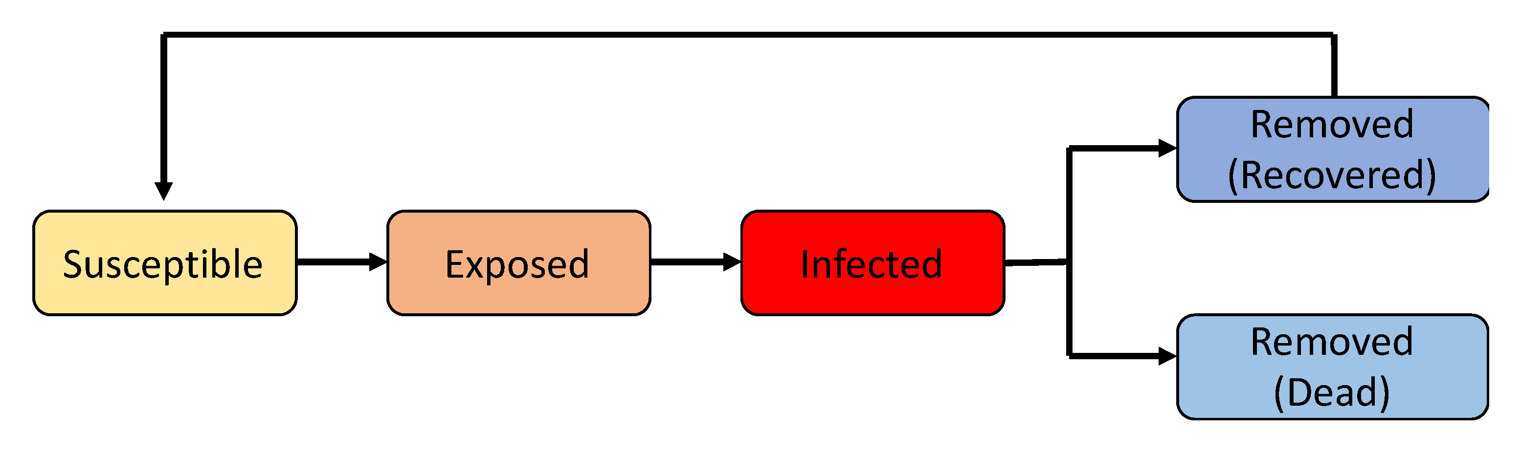
A SEIRS model classifies people into categories: susceptible (S), exposed (E), infected (I), eliminated from the susceptible population (R), and potentially back to susceptible (S) again, depending on whether a person recovered has immunity from the disease (
Figure 1). The modeler’s job is to define the equations that determine how people move from one category to the next. Those equations depend on a wide variety of parameters drawn from biology, behavior, politics, economics, climate, and more [
14].
The SEIR model (used in Wuhan), structured by stages, was adapted to simulate the outbreak in Lima over a period of one year. One of the implications of this method is to ignore all demographic changes in the population (births, deaths, and aging).
We divided the population into susceptible (S), exposed (E), infected (I) and recovered (R) according to the state of infection, and according to age in bands from 0 years to 80 years, and a single category of age 80 and over (resulting in 9 age categories). Susceptible people can acquire the infection at a certain rate when they come into contact with an infected person and enter the exposed disease state before becoming infectious and then recovering or dying.
We assume that Lima is a closed system, during this epidemic the population remains constant at 9.5 million (that is, S + E + I + R = 9.5 million). Given a certain number of infected individuals in a population, the mixed pattern of individuals of a specific age in age group “i” will change their probability of exposure to the virus.
We incorporate contributions from asymptomatic cases; where the transmission capacity is high. For a given age group “i” (age category by ten year bands), epidemic transitions can be described by:
where
β is the transmission rate (scaled to the correct value of
R0),
Ci,j describes the contacts of age group
j made by age group
i, κ = 1 − exp (−1/dL) is the probability daily exposure of an individual who becomes infectious (where dL is the average incubation period) and
γ = 1 − exp (−1/dL) is the daily probability that an infected individual recovers when the average duration of infection is dL. We also incorporate contributions from asymptomatic cases, 1 −
ρi denotes the probability that an infected case is asymptomatic. We assume that younger individuals are more likely to be asymptomatic and less infectious (infectivity ratio compared to
Ic,
α) [
13].
Interventions and Social Interaction
Patterns of social interaction vary across locations, including homes, workplaces, schools, and other places. Therefore, we use the method established by Prem and colleagues, which takes these differences into account and derives the location-specific contact matrices (C) for different scenarios. In a normal setting, contacts made at all of these locations contribute to the overall pattern of interaction in a population, so we sum the contacts at the different locations to get our reference contact [
15,
16].
According to the state of infection, we divide the population into susceptible (S), exposed (E), infected (I) and recovered (R) individuals. An infected individual in an age group can be clinical (Ic) or asymptomatic (Isc), and
ρi refers to the probability that an individual is asymptomatic or clinical. The age-specific interaction patterns of individuals in age group
i,
Ci,j alter their probability of being exposed to the virus given a certain number of infected individuals in the population. Younger individuals are more likely to be asymptomatic and less infectious, that is, subclinical. When
ρi = 0 for all
i, the model simplifies to a standard SEIR. The infection force
φi,t is given by 1 – (
), where
β is the transmission rate and
α is the proportion of transmission that results from a subclinical individual. SEIR = susceptible-exposed-infected-recovered [
14].
In the outbreak of the epidemic, different intervention strategies aim to decrease social interaction in different contexts to reduce the general spread in the population. To simulate the effects of interventions designed to decrease social interaction, comprehensive connection matrices are created for each intervention scenario. From these building block matrices, the following three scenarios are considered:
- -
First scenario, (theoretical): It was assumed that the shape of social interaction patterns has not changed in all types of places or locations, students go to classes and people work normally (without quarantine interventions).
- -
Second scenario, partial quarantine: intense control measures were assumed in Peru to contain the outbreak, schools and universities were closed, but then the partial quarantine was lifted on May 10 until the 90-day simulation was completed.
- -
Third scenario, rigid quarantine: it was assumed that there are social distancing control measures, school and university students did not have any contact because they were isolated taking classes online and people worked remotely, and approximately 12% of the workforce (health care personnel, police and other essential government personnel) would be working even during the control measures, but then the quarantine is lifted on June 30 until the simulation period is completed.
For the third scenario, we simulated the effects of the strict control measures that ended in early July, and allowed a staggered return to work while schools and universities remained closed, that is, 25% of the workforce working in the weeks one and two, 50% of the workforce working in weeks three and four, and 75% of the workforce is working.
2.3. Simulation by Agents
To construct the agent-based simulation model, this study adopted the models and indicators proposed by [
13,
15]. The proposed model by [
13] investigate the effect of implementing different strategies to decrease social mixing in Wuhan, China, to decrease COVID-19 cases. The model proposed by [
15] constructed an agent-based simulation model to explore the COVID-19 cases in Argentina. However, the proposed model in this study is a multi-agent based model that can visualize the emerging dynamics of the interaction of various social and biological factors during the development of the COVID-19 pandemic in Peru.
As listed in
Table 1, the following parameters will be analyzed in the model:
Among the indicators proposed in the model, 98% have been taken for programming due to the limitations in accessing official information; however, we consider that enough have been taken to project the scenarios, pending the completion of new inquiries for future research. In addition, due to the public debate regarding Face-to-face assistance to colleges and universities in 2021, a fourth scenario was considered to analyze its impact.
2.4. Simulation Implementation
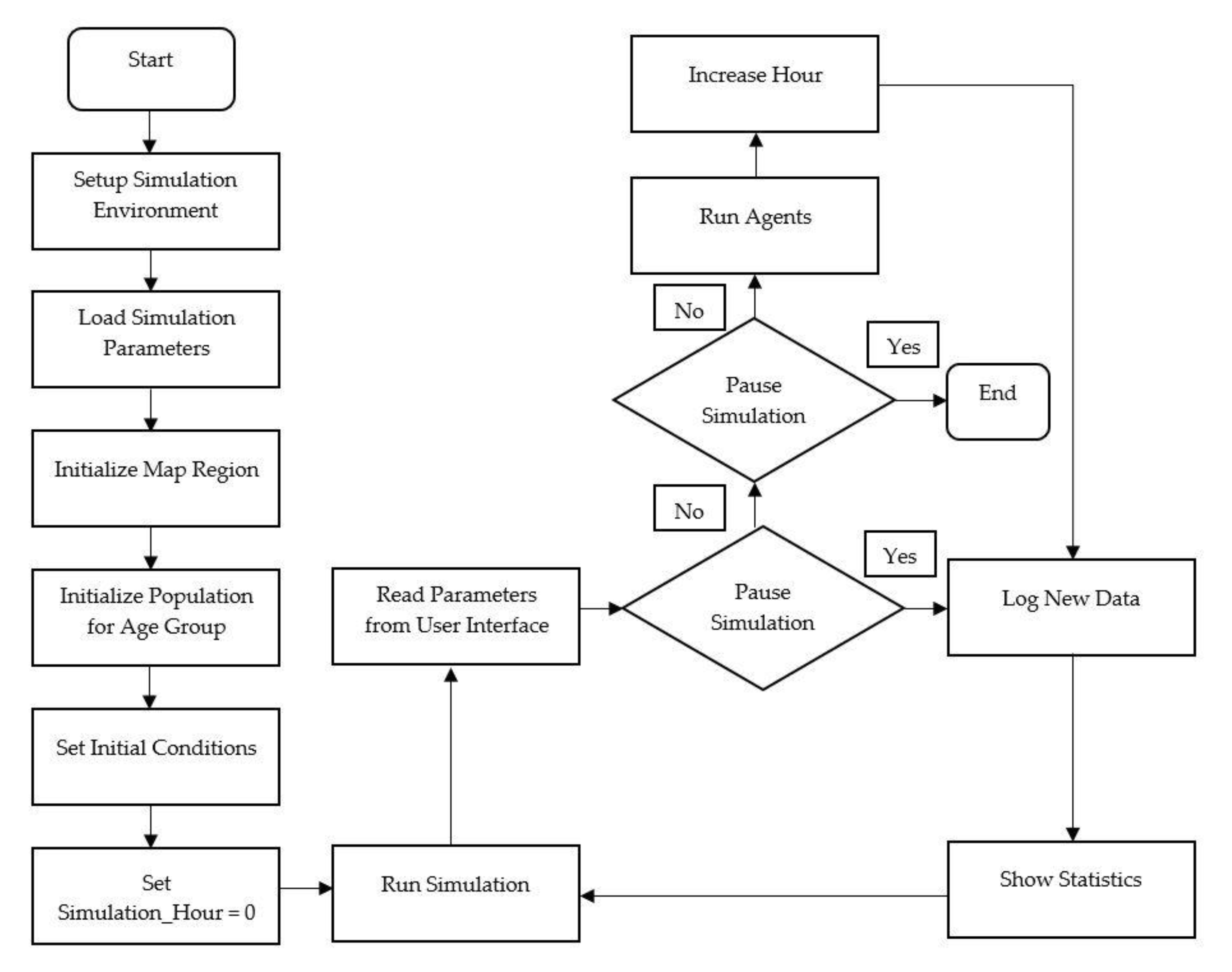
This section describes in pseudo-code how this model is implemented in the NetLogo environment (Adapted from Jiménez’s model [
13].
Figure 2 shows the flow diagram of the simulation execution.
The general structure of the model according to Jiménez can be summarized as follows (Interaction Rules):
- -
The NetLogo simulation environment is started including the virtual world area where the map of the Peruvian territory and the agents that represent the Peruvian population during the pandemic are shown.
- -
The parameters are initialized with the initial conditions and the modeling time is started with the command simulation_hours = 0.
- -
The simulation runs in a loop where each tick or iteration is equivalent to 1 h.
- -
After the modification, some parameters configured in the graphical interface will have a real-time impact on the behavior of the agents, and therefore will have a real-time impact on the results obtained.
- -
To make it easier to fix the parameters in real time, the simulation can be paused while the required parameters are being adjusted and then continue to run with the new values.
- -
The graphical interface shows the current values and records the data for later analysis.
- -
The simulation time is increased by one hour.
- -
The simulation orders all the agents to act
- -
The simulation loop is repeated until the user commands through the graphical interface to terminate the execution. The number of iterations can also be determined through the NetLogo command interface (observer command line) or by using the Behaviour Space for experiments requiring multiple runs with different parameters.
2.5. Geographic Delimitation of the Area of Impact by COVID-19 in Peru
Jiménez recommends that a map of the territory should be digitally represented in the simulation in png format, in this case we define the study area in white in Peru, while the area excluded from the analysis is in black, and, the main axes of circulation in yellow (streets, routes, etc.). The reference to the digital map that indicates the study area must be indicated in setup-globals > ifelse load_city_map > import-pcolors (
Figure 3).
2.6. Study Area with Population Density Adjustment
It is necessary to obtain the number of square meters per inhabitant of the geographical area to be inspected. If the density is expressed in number of inhabitants per square kilometer [
4], then:
Taking into account the value M
2 inhabitant, the total number of logical patches (Plogs) necessary to model a population of N groups of agents was calculated:
In the simulation, the TotalPlogs value is modified by multiplying the vertical (Vres) and horizontal (Hres) resolutions of the habitable modeling area (white patches) by the parameter meters_per_patch (M
Patch). In this case the value of M
Patch is obtained as follows:
For the Peruvian territorial model that was examined, it turned out that on average 4009 m
2 per inhabitant correspond (calculated from the data available in the 2017 census in Peru) with a rectangular resolution of 530 vertical patches × 540 horizontal patches (286,200). Obtaining the following parameters for a population of 21,050 agents:
With TotalPlogs = 84,389,450, the required M Patch value is calculated: M × Patch = 84,389,450/(540x 530x) = 84,389,450/286,200 × 2, obtaining M Patch = 10 for a population of 21,050 agents with 4009 m2 per inhabitant.
2.7. Demonstration of the Evolution of the Model
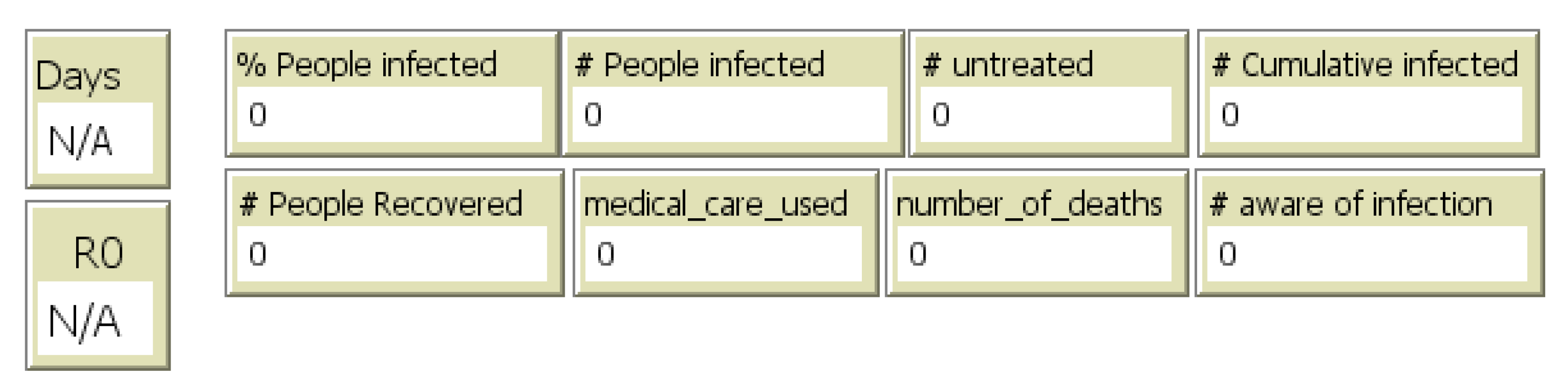
The simulation allows users to examine the development of the infection and the impact on the population over time. When executing the model, the evolution indicators shown in the interface (
Figure 4) are the following:
Days: number of days elapsed since the simulation started, number of reproduction (R0), percentage and number of infected people, untreated cases of infected people, infected people receiving medical care, recovered people, deceased people and medical care used: number of hospital beds used [
13].
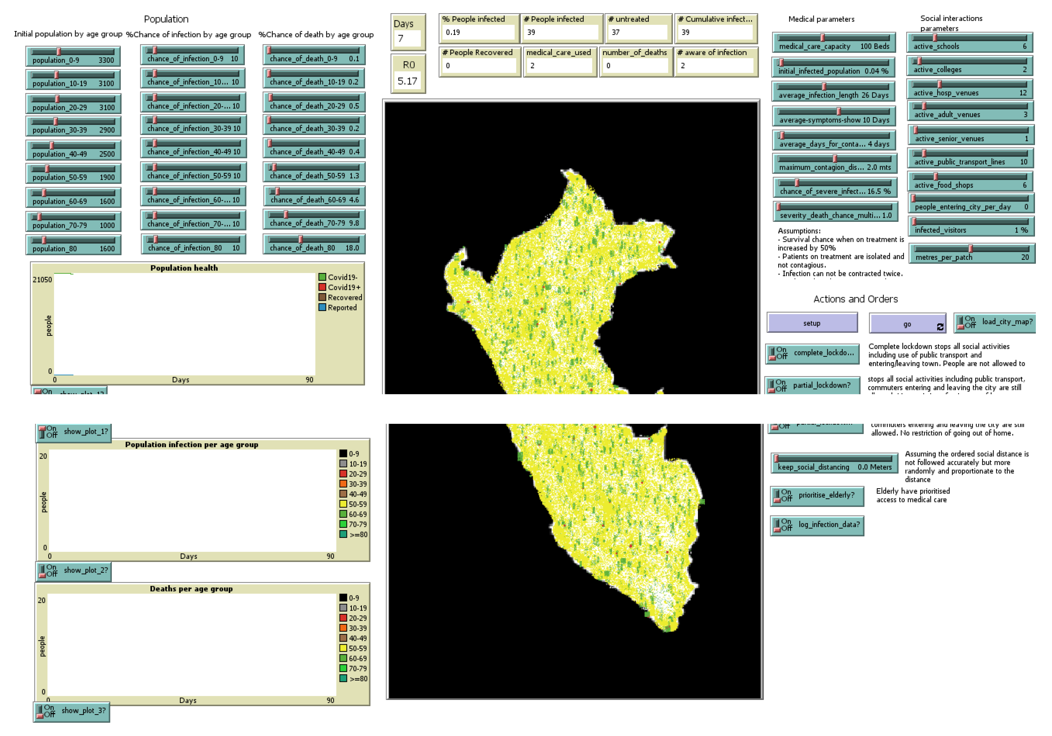
Each iteration or tick of the simulation represents one hour. Infected people are represented by red dots on the map. Uninfected people are represented by green dots. When the simulation is running, the group of green dots will appear and dissipate. These correspond to social gatherings of simulated individuals of different age groups in different types of sites or places, and activities during the day. Individuals using public transportation are grouped mainly along the yellow lines on the map (
Figure 5) [
13].
Figure 5 shows a general image of the computer system of the COVID-19 simulation model that will help us to present the results.
3. Results
To model the behavior of COVID-19 in Peru, the experience of the Argentine model was considered as the most similar to our reality. There is much difficulty specifying the official data on COVID-19 in Peru. For this simulation, a sample of 21,050 agents was considered and it was divided into an age group of 10 years according to the real population distribution according to the National Institute of Statistics and Informatics (INEI). As we are using a sample of population instead of a total sampling, it is important to mention at this point that the results obtained will not be absolute, but the evolution of the temporal trends and the daily growth rates of reported infected.
Proportional distribution of the population according to age group can be seen in
Table 2:
In Peru, the government and the health sector have regulated avoiding public gatherings, staying home more frequently, and staying away from others. If people are less mobile and interact less with each other, the virus has less chance of spreading.
Peru’s socioeconomic activity, based on informal work management, means that people have refused to comply with the government’s provisions and go out to seek daily survival, increasing the level of infections and deaths from COVID-19. In sectors of the upper-middle class, social distancing measures and mobility restrictions have been complied with.
In this way, three possible scenarios for the evolution of COVID-19 in Peru are analyzed. In all cases, the starting point was 8 infected people out of the 21,050 agents that make up the population sample.
3.1. Scenario 1 (Reference)
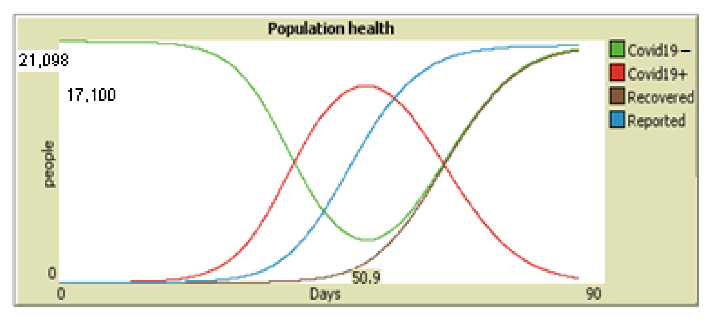
First scenario: No type of restriction is applied throughout the period considered. It begins by considering 8 infected people, and the partial_lockdown option (Partial_Lockdown = false) is deactivated, indicating in this case that there is no quarantine and no minimum social distance.
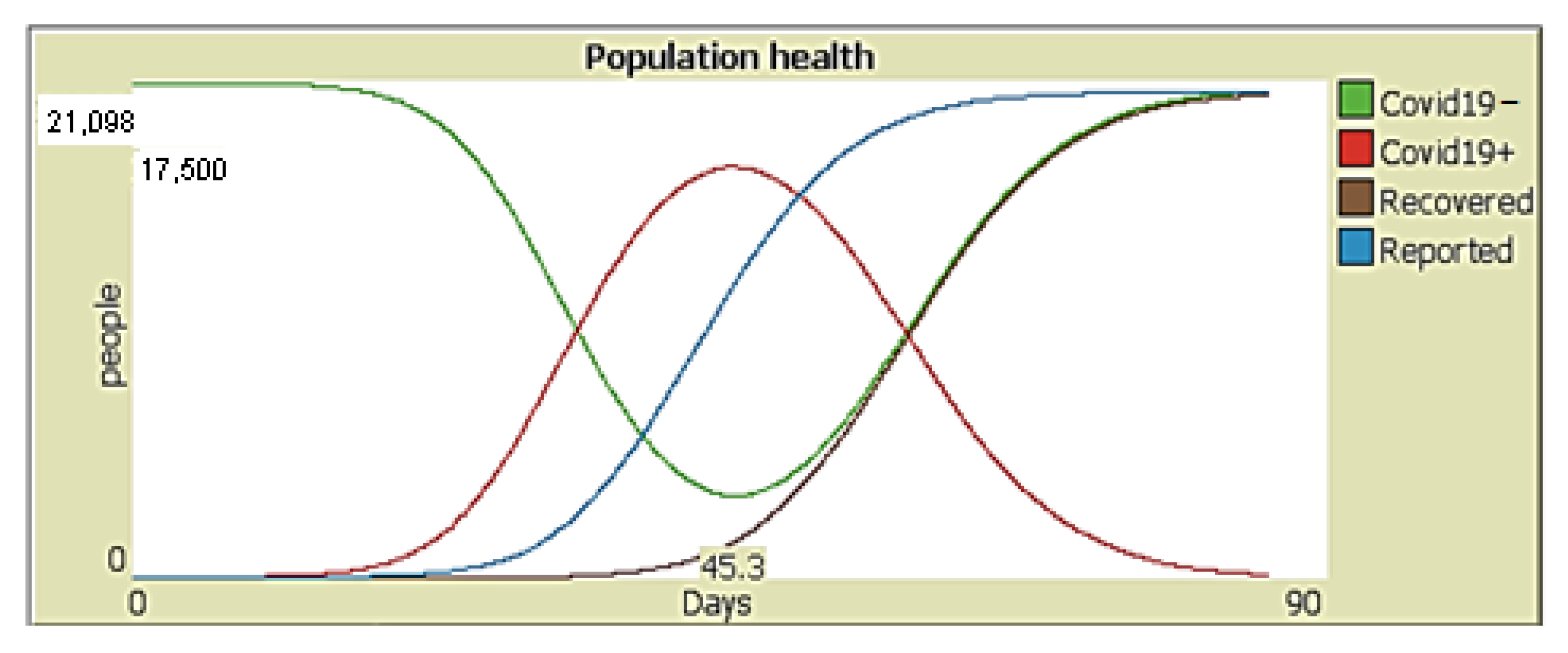
Figure 6 shows the dynamism of the virus for a period of 90 days, with four classifications in the population, the green line represents the agents with negative COVID-19 test, the red line represents the agents with positive COVID-19 test, the brown line represents the cases recovered, the blue line represents the reported cases.
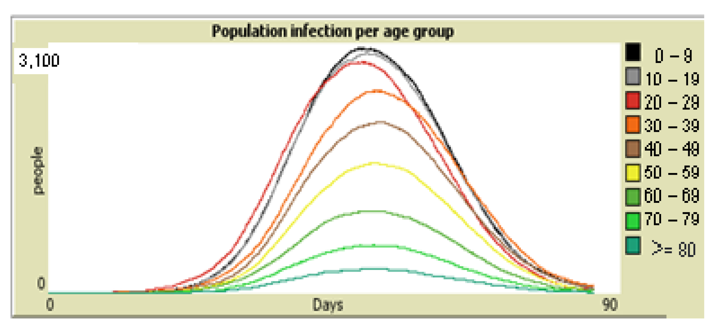
Figure 7 shows the infected population by age group, according to ten year age bands from 0 years to 80 years, and a single age category of 80 years or more (resulting in 9 age categories). The results of the simulation analysis shows that in a period of 90 days, young people from 0 to 49 years old are the most infected.
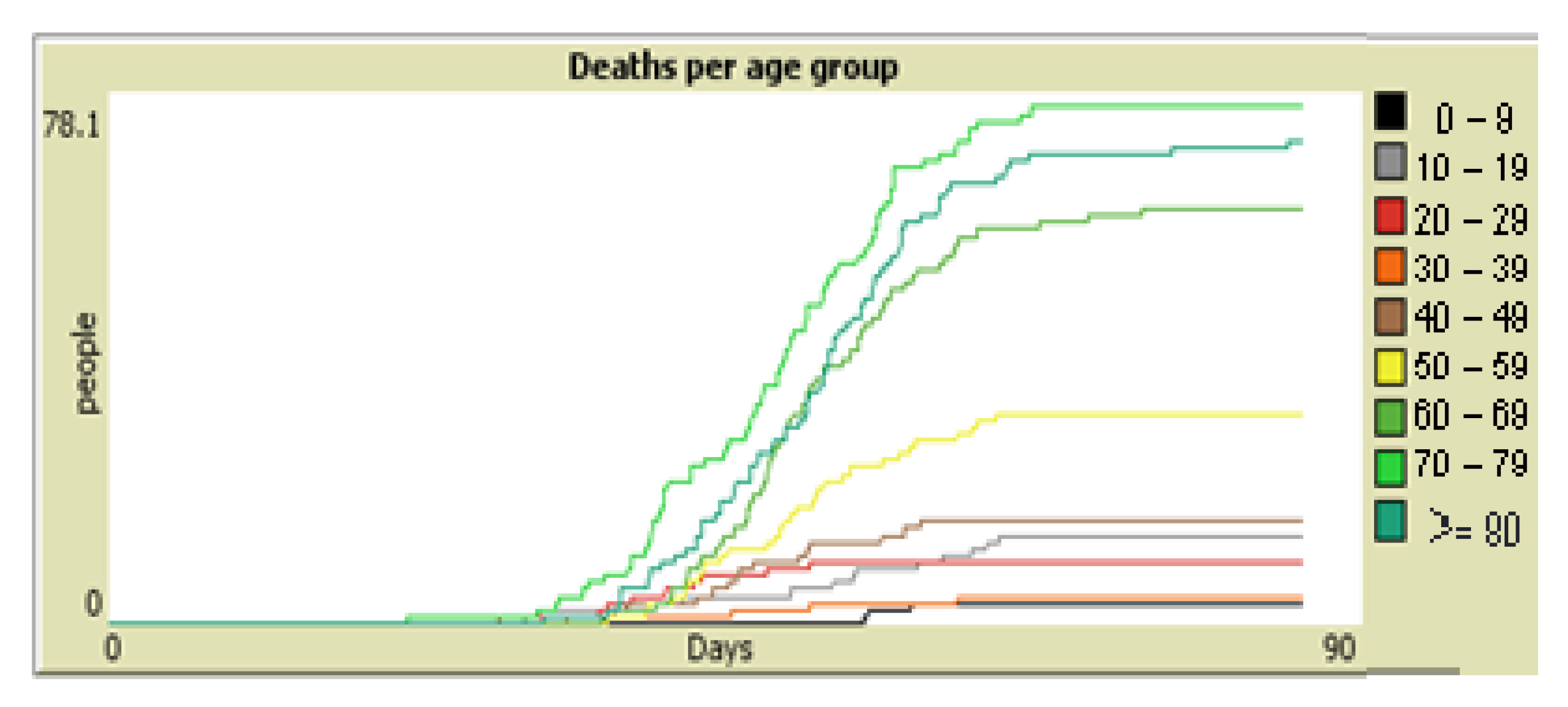
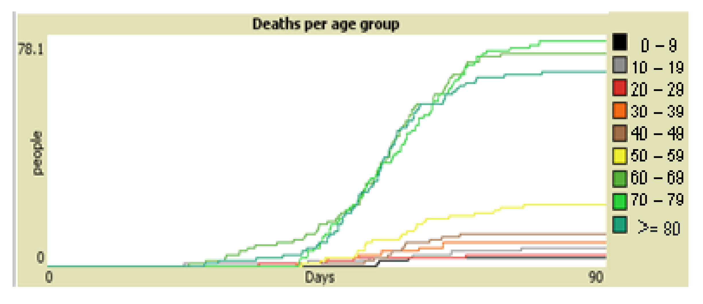
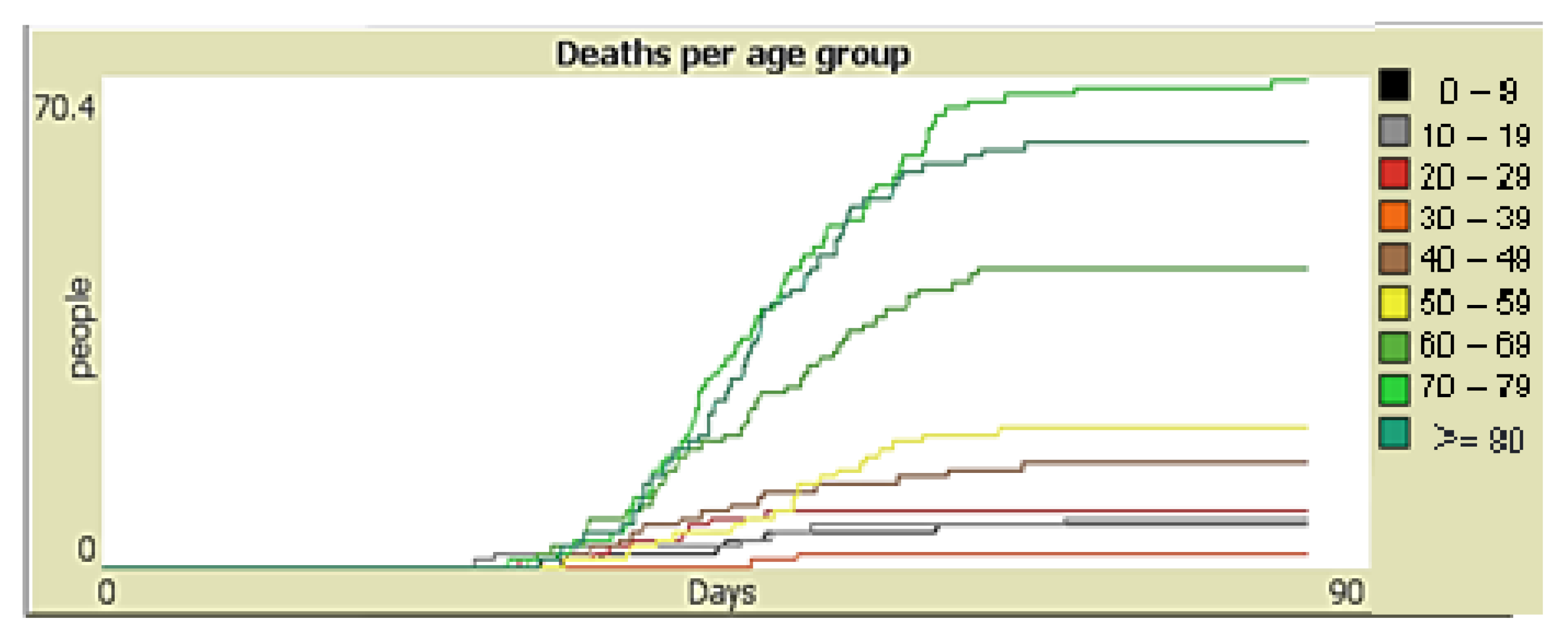
Figure 8 has the same parameters as
Figure 7 and shows the cases of deaths based on different age groups. The main goal of this analysis is to identify the COVID-19 related deaths for different age groups in a span of 90 days. As depicted in
Figure 8, adults over 60 years of age are the most affected by the mortality of the virus. According to the three figures of the first scenario, an increase in infected people of 65% can be seen.
3.2. Scenario 2
Second scenario: Start with 8 cases of infected people that after 16 days become 177 cases of infected people and then the quarantine conditions are introduced. At that time, the country’s quarantine is activated (Partial_Lockdown = true) in order to simulate the quarantine conditions implemented in Peru. The restrictions are maintained until day 90 of the simulation is reached.
Figure 9 shows the dynamism of the virus, with four classifications in the population, the green line represents the agents with negative COVID-19 test, the red line represents the agents with positive COVID-19 test, the brown line represents the cases recovered, the blue line represents the reported cases.
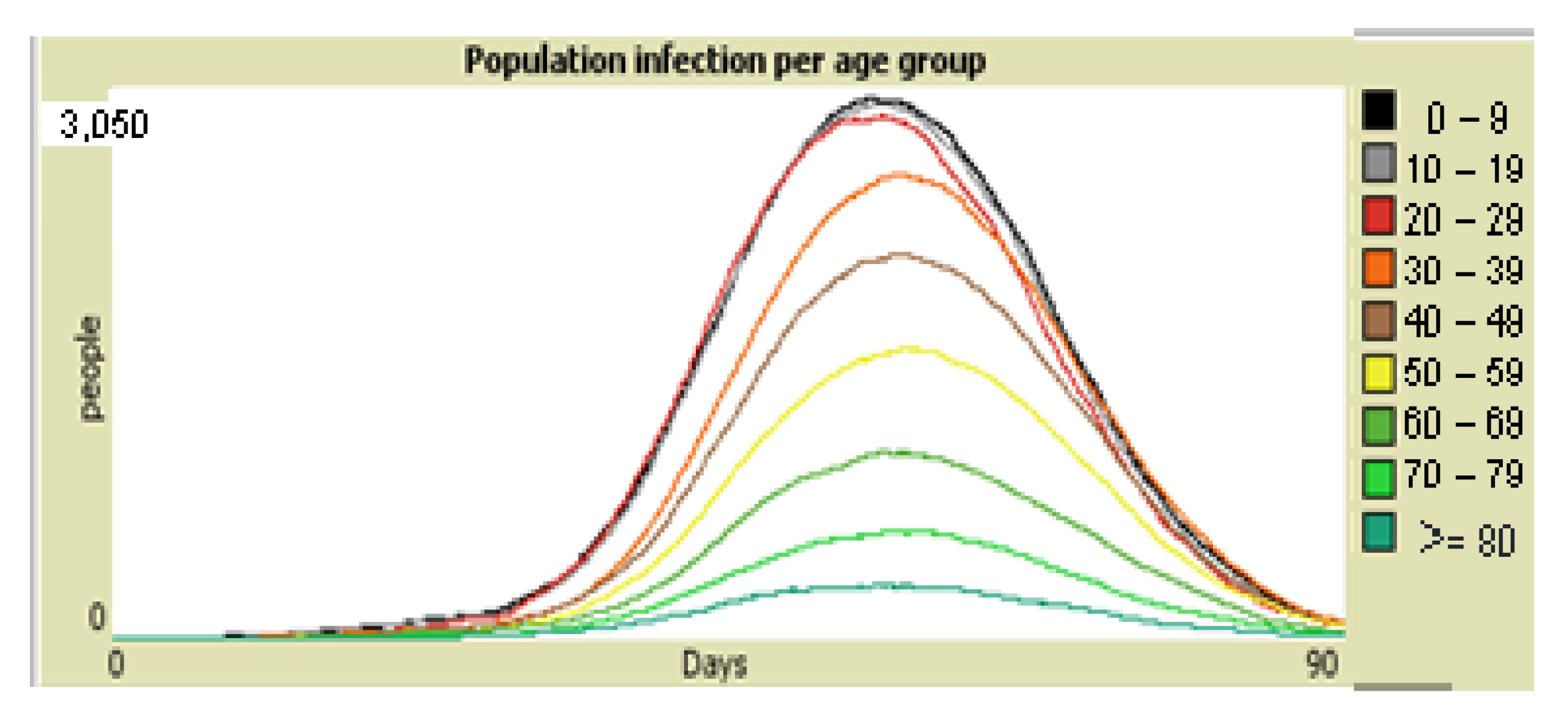
Figure 10 shows the infected population by age group, according to ten year age bands from 0 years to 80 years, and a single age category of 80 years or more (resulting in 9 age categories). The simulation model starts from day 0 to day 90 and when the simulation run end in day 90, the results shows although there is a decrease in contagion with respect to scenario 1, the group that is most contagious is from 0 to 49 years old.
Figure 11 has the same parameters as
Figure 10 and shows the cases of deaths by age groups. Similar to previous simulation runs, the simulation results for 90 days shows that adults over 60 years of age are the most affected by death from the virus.
According to the three figures of the second scenario, there is an increase in the number of infected people of 23%.
3.3. Scenario 3
In the third scenario, the time span for the simulation model was changed from 0 to 90 days to 0 to 176 days. The 177 cases are reached on day 20 of the simulation, starting from the initial conditions mentioned above. At that time, there is a staggered quarantine of the country (Partial_Lockdown = true) with the use of masks and minimum social distancing (KSD) of 1.5 m mandatory. With the purpose of simulating the quarantine conditions implemented in Peru, the restrictions indicated are maintained throughout the period considered in the simulation.
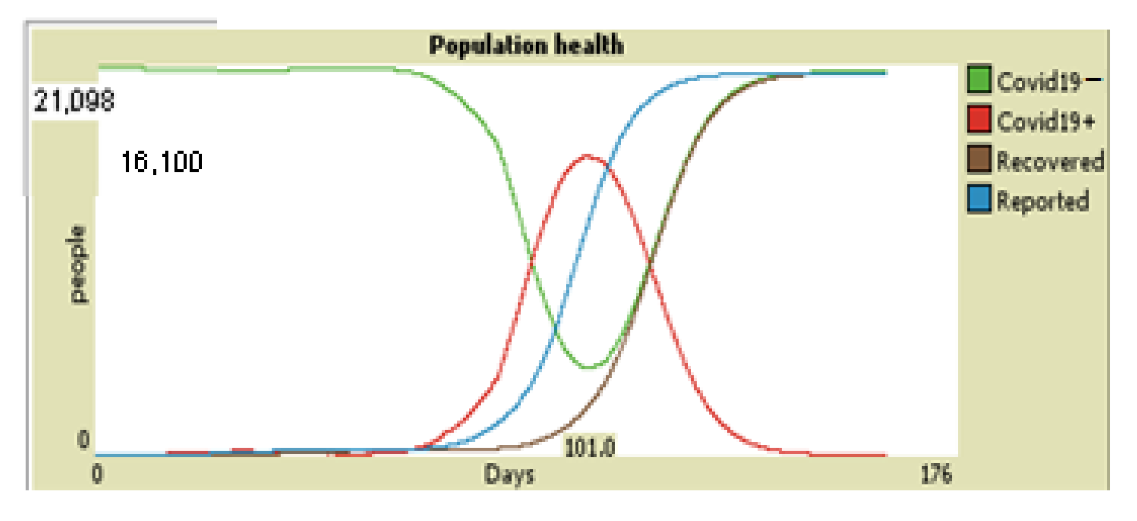
Figure 12 shows the dynamism of the virus, with four classifications in the population and the simulation model was run for 176 days. The green line represents the agents with negative COVID-19 test, the red line represents the agents with positive COVID-19 test, the brown line represents recovered cases, the blue line represents reported cases.
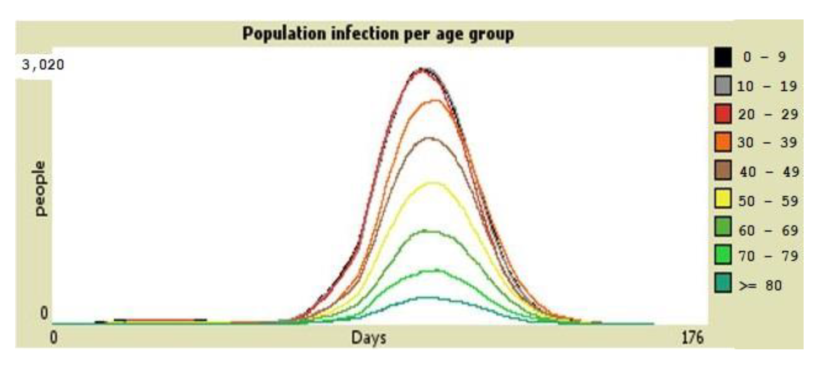
Figure 13 shows the infected population by age group for 176 days, according to ten year age bands from 0 years to 80 years, and a single age category of 80 years or more (resulting in 9 age categories).
Figure 14 has the same parameters as
Figure 13 and shows the cases of deaths by age groups. The results of the simulation, which ran for 176 days, show that adults over 60 years of age are the most affected by the virus.
Based on the three figures of the third scenario, an increase in infected people of 37% can be seen. The simulations were random. That means the results for each were unique to your reading of this article; if you scroll up and rerun the simulations, your results will change by approximate values. Even with different results, extended social distancing generally works better.
3.4. Scenario 4
Scenario 4 for the outbreak of the epidemic (face-to-face assistance to colleges and universities in 2021). In this scenario, the level of contagion is simulated if face-to-face education is resumed in colleges and universities in March 2021. In the simulation for 90 days, an increase in the number of infected population of 65% can be seen.
For a period of 90 days,
Figure 15 shows the dynamism of the virus, with 4 classifications in the population, the green line represents the agents with negative COVID-19 test, the red line represents the agents with positive COVID-19 test, the brown line represents recovered cases, the blue line represents reported cases.
Figure 16 shows the infected population by age group, according to age in categories from 0 years to 80 years, and a single age category of 80 years or more (resulting in 9 age categories). In this scenario, we can see an increase in infected people in the ages 0 to 19 years within 90 days.
Figure 17 has the same parameters as
Figure 16 and shows the cases of deaths by age groups. The simulation results illustrate that within a period of 90 days, adults over 60 years of age are the most affected by death from the virus.
3.5. Confidence Intervals
Each modeling approach relies on a series of simplifying assumptions that both empower and limit it. This allows us to quickly explore a wide range of scenarios, quickly obtain analytical approximations of some regimes, etc. To address these limitations, we moved to a stochastic approach [
13,
18].
The SEIR model simulations generate a large amount of data on each set of parameters, so we need a way to accurately summarize the results of all the simulations. This is done by reporting the median (or mean) value at each time step, along with the 95% confidence interval. In this way we can get a clear picture of the range of possible values that can be observed in the real world.
Since we are interested in what happens when we have an outbreak or epidemic, before calculating the median and confidence interval, we remove all executions that did not cause an outbreak. This is equivalent to reporting the size of the outbreak on the condition that there is a large or significant outbreak.
Despite its relative simplicity, there is a great deal of intrinsic and unavoidable uncertainty in this type of process, which limits our ability to accurately forecast the number of infected individuals. However, we can accurately model the main characteristics of the spread of the epidemic, as well as the effects of the proposed containment and mitigation measures [
13].
Different models have different degrees or levels of uncertainty, but it is impossible to eliminate it completely, so we must always report the confidence interval for any number that we report. With a population sample mean of 2339.11 and a sample size of 21,050 agents. The values of x = 2321.99 and y = 2356.22 refer to the lower and upper values of the 95% confidence interval. The random or stochastic method that we present in this project brings us one step closer to the real world, allowing us to obtain a more realistic description or image of not only what is most likely, but also what is possible.
4. Discussion
As shown in the simulation results, the movement of the graphs in the first (reference) scenario where no restriction measures were taken, it is possible to appreciate the severity of the contagion by COVID-19, which is critically harmful to the population since in 120 days would have quickly infected 65% of the population, having created a very serious crisis due to the saturation of hospitals, lack of medical personnel, lack of medicine and intensive care equipment. However, where restrictive measures are taken in the second scenario, it turns out critically well, since, in 90 days, 23% of the population is infected, slowing down the spread of the virus for a few days, allowing in some way better conditions of care in hospitals, forcing the population to a sharp reduction in social mobility for a longer time.
According to the third scenario, the graph comes out critically acceptable, since in 210 days, 37% of the population is infected, slowing down the spread of the virus for a longer time, this is because the quarantine is staggered. It is considered that all this is observed with a sample of the population. While the simulation results in the fourth scenario, suggests that if face-to-face education is resumed in colleges and universities, the regrowth will increase significantly to 65%.
In Peru, the majority of school-age children and adolescents are poor and transportation is precarious. Many have to travel considerable distances, thereby increasing contagion. Therefore, extreme measures must be taken to avoid contagion of children, which would increase the complexity of hospitalizations of children and parents. Mass vaccination is an important factor for returning to face-to-face classes.
As depicted in
Figure 7,
Figure 10 and
Figure 13, among the infected population based on different age groups, the most infected are young people, as they have greater social interaction. These graphs are closely related to the health graphs of the population (
Figure 6,
Figure 9 and
Figure 12), repeating these similar circumstances for both the second and third scenarios. Furthermore, the simulation results in
Figure 8,
Figure 11 and
Figure 14 demonstrate that the elderly are the most affected, as they have a lower probability of surviving the contagion of the virus. These graphs are closely related to the health graphs of the population (
Figure 6,
Figure 9 and
Figure 12), repeating these similar circumstances for both the second and third scenarios. Finally, it can be seen from the graphs presented that if the days of quarantine increase, the probability of becoming infected with the virus decreases, and the slowdown in the contagion of the virus increases, therefore, it can be concluded that, if the mobility of agents, the increase in contagion decreases while the quarantine is less and less.
4.1. Research Contribution and Future Direction
This study presents a basic model, the first of its kind created to model the Peruvian reality and it has a great capacity for extension and future research. In contrast, mathematical SEIRs are difficult to extend. For example, possible extensions include: (i) considering different parameters and indicators to obtain different results, (ii) precise geolocation using cell phone data, (iii) cultural and social effects typical of Peruvian populations and particular situations to the national reality such as those that gave rise to the “exodus of hunger”, (iv) interactions with economic models to jointly study the severity of the pandemic with the related economic consequences.
Extensions to this base model will allow the exploration of measures and policies in relation to COVID-19 in simulations, allowing officials to be in a position to evaluate these policies and to see the consequences of measures before implementing them. This is important because due to complexity, policies and measures often have unexpected or often counterproductive consequences. This model is designed for the exploration and discussion of this type of COVID-19 policies in Peru.
4.2. Conclusions
In conclusion, by simulating greater social distancing, it can be seen that less contagion will be in the population, slowing down the virus, as people exposed to COVID-19 are not only more likely to get sick, but also more likely to spread the disease.
The agent-based model applied in this case allows us more information on the inquiries between the virus and human beings, allowing us to take more assertive measures. The lack of data available to the research centers has been a restriction for the simulation by agents, which is why it is only an investigative study.


 ,
, 


