
Efficiency of Energy Exchange Strategies in Model Bacteriabot Populations


Abstract
1. Introduction
2. Literature Review: Teamwork in the World of Small-Scale Systems
2.1. Interaction Between Artificial MRs/NRs
2.2. Interaction Between Living MRs/NRs
2.3. Efficiency of Exchange Strategies
2.4. Previous Works
- –
- We introduce a parameter that regulates the extent to which the fitness of the organisms to the environment affects their ability to grow and reproduce (parameter ) and study the influence of this parameter on the survival rate of populations;
- –
- We introduce a mechanism that regulates the frequency of energy exchange events between organisms in a model population (parameter ) and study how this frequency affects the survival rate of this population under different energy exchange strategies;
- –
- The volume of computational experiments is increased significantly to obtain more detailed and reliable results;
- –
- Enhanced data visualization and additional statistical analysis are used to demonstrate the influence of the energy exchange factor on the survival rate of the populations.
3. Materials and Methods
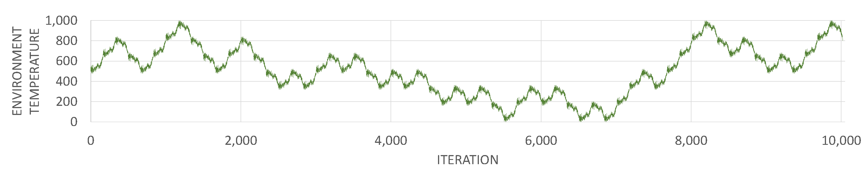
3.1. Environment
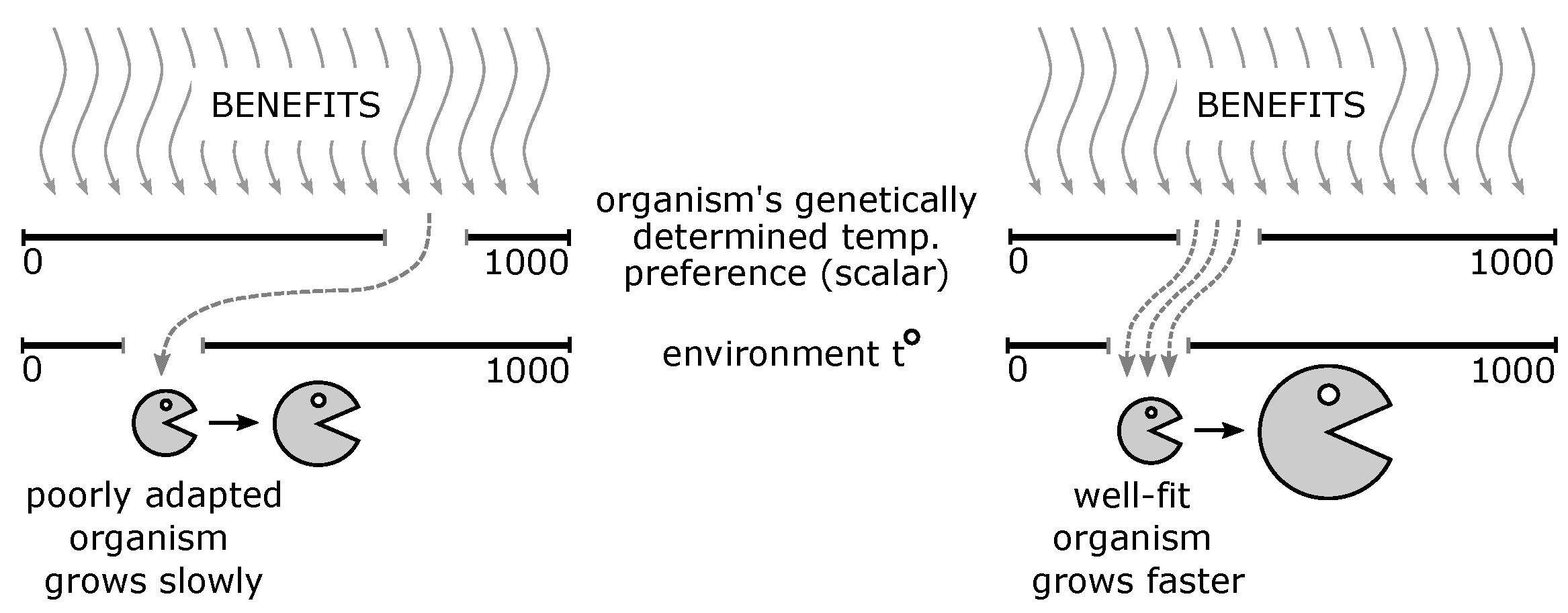
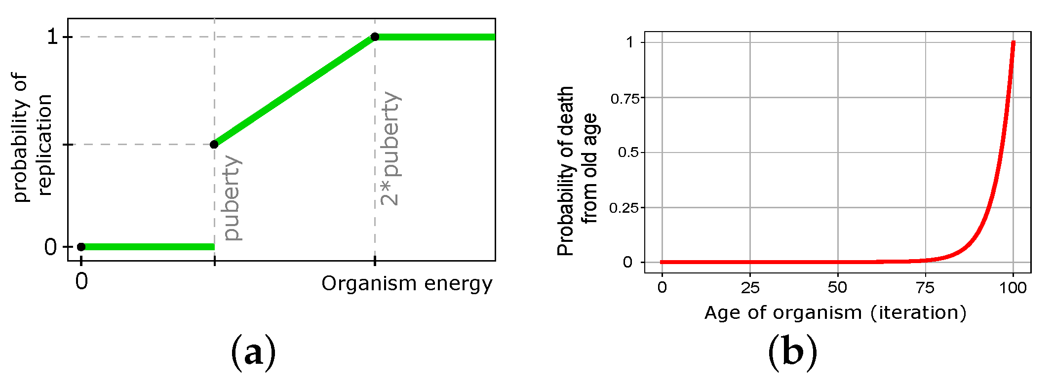
3.2. Organisms
3.2.1. Organism’s Structure
3.2.2. Organism’s Actions
3.3. Computational Experiments
- -
- -
- : The maximum allowed deviation of the temperature preference (TP) of descendants from the TP of their ancestor (see (4));
- -
- : The frequency of interactions among organisms. The regulation of this parameter allows us to study the behavior of the system for different ratios between the speed of growth and the intensity of energy exchange;
- -
- : The extent to which the organisms’ fitness to the environment affects their growth (see (2));
- -
| Algorithm 1 Pop_Survive |
Input: Output: True (1) or False (0)
|
3.3.1. Variation Ranges of Independent Parameters
- The parameter controls the energy supply to the system. In our experiments, it takes values from the set , which consists of the following three ranges:
- –
- From 0.01 to 0.5 in increments of 0.01;
- –
- From 0.55 to 1 in increments of 0.05;
- –
- From 1.1 to 2 in increments of 0.1.
Values below 0.01 do not allow the system to provide enough energy for the populations to survive. Preliminary experiments showed that with , the death mechanics withdrew more energy from the population than the growth mechanics provided, so the populations died out regardless of the values of the other independent parameters. On the other hand, values of make the energy flow into the system excessively abundant, so that all other independent parameters have almost no effect on the survival of the populations. Note that we use a denser grid for small values of to study the situation of scarce energy in more detail, which seems to be of most interest in practical applications. - The parameter controls the mutation rate. In our model, it regulates how far the temperature preference of the descendant can deviate from that of the ancestor. In the experiments, takes values fromAlthough values of below 0.015 are more realistic, we have to consider higher mutation rates for the system to be able to evolve observably in a relatively short time (≈10,000 iterations). Values above 0.5 hardly fit the concept of evolution as a gradual process.
- The parameter regulates the number of interactions among organisms per iteration. It takes values fromValues of below 0.07 make the interactions so rare that the model fails to provide enough data to serve its main purpose—assessing the efficiency of different energy exchange strategies. Values above 0.5 involve more than 50% of all possible pairs in the system in interaction (see step 2(d) in the algorithm Pop_Survive). Such a high rate is hardly consistent with the idea of an algorithm iteration as a relatively small discrete unit of time, which is desirable to follow the development of the system gradually.
- The parameter controls how sensitive the growth of the organism is to the fitness of this organism to the environment (the higher , the stronger the response). In our experiments, takes values fromIt has been experimentally shown that the values change the behavior of Δ (see (2)) only slightly compared to .
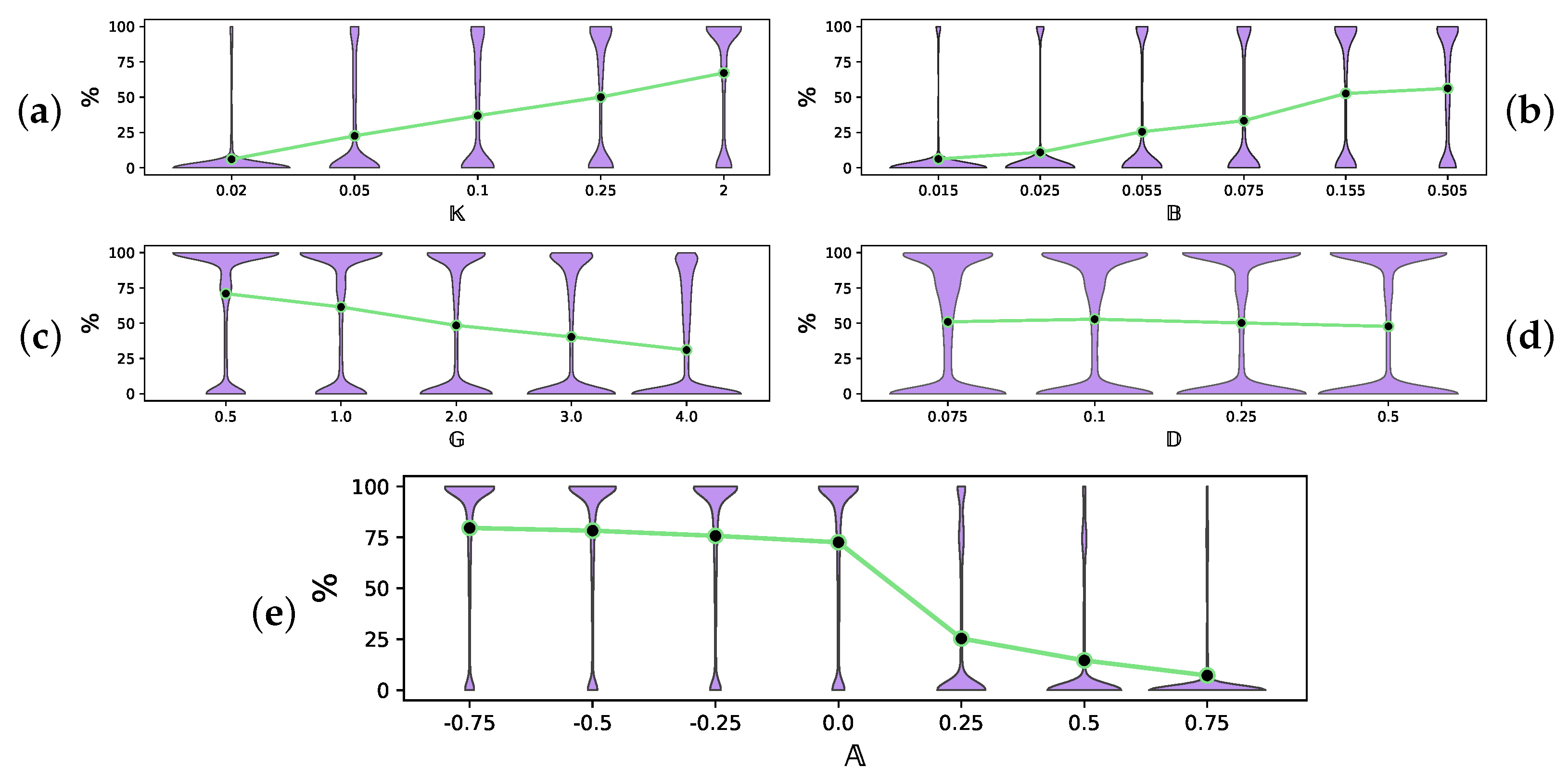
- The parameter , the central parameter for this study, controls the “selfishness” of the agents. In our model, takes values fromcovering the entire spectrum of energy exchange behavior, from the explicit robbery of weaker agents to indifference and the explicit sharing of energy with weaker agents.
- Favorable if ;
- Ambiguous if ;
- Unfavorable if .
3.3.2. Scientific Constants
4. Results and Discussion
4.1. Dependence of Survival on Starting Conditions
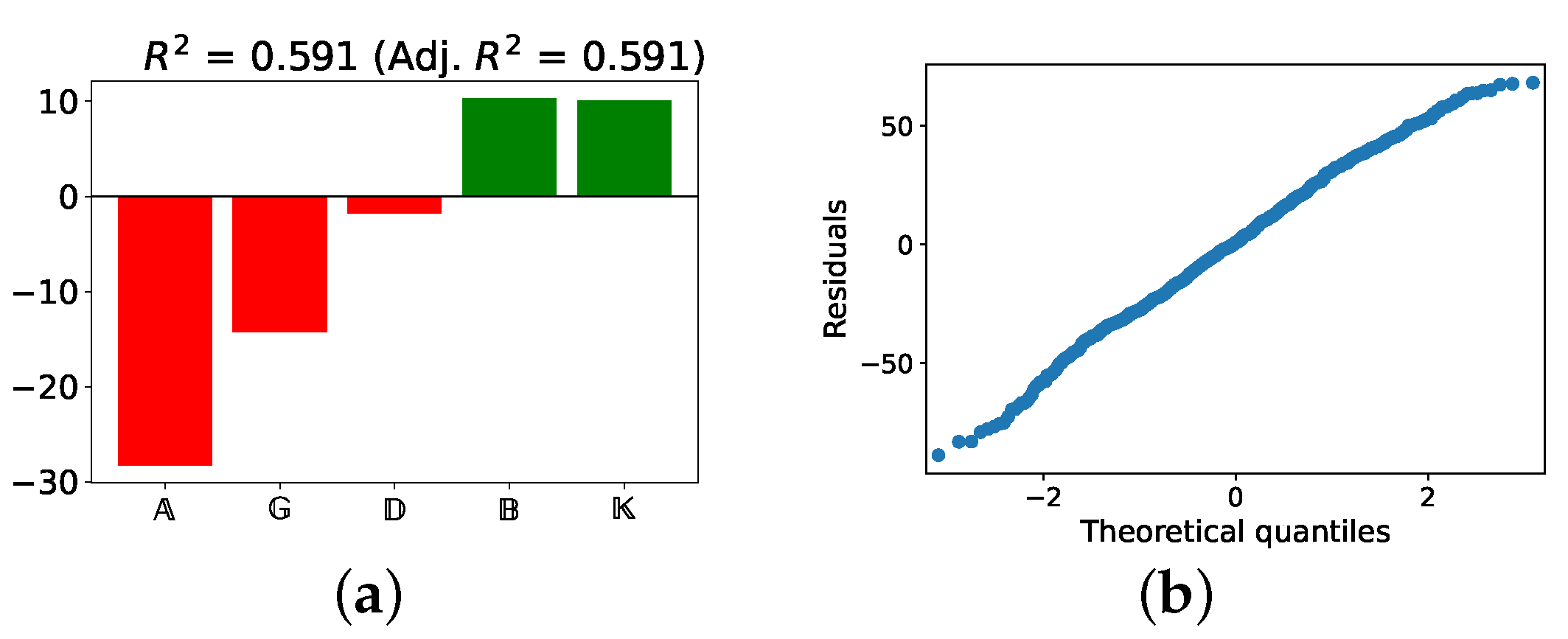
4.1.1. Linear Model
4.1.2. Importance of Variables
4.2. The Effect of Altruism in Different Experimental Settings
4.3. Visualization of Raw Results
5. Conclusions
Author Contributions
Funding
Institutional Review Board Statement
Informed Consent Statement
Data Availability Statement
Conflicts of Interest
Appendix A. Visualization of Raw Results of Experiments

| ∖ | 0.07 | 0.1 | 0.25 | 0.5 |
|---|---|---|---|---|
| 0.5 | 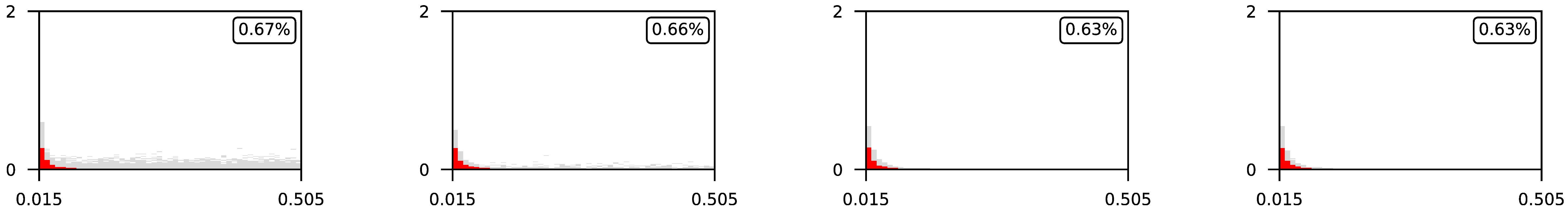 | |||
| 1 | 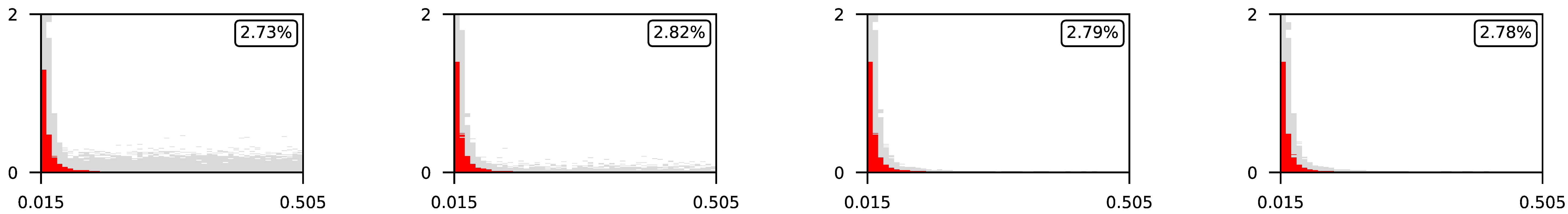 | |||
| 2 | 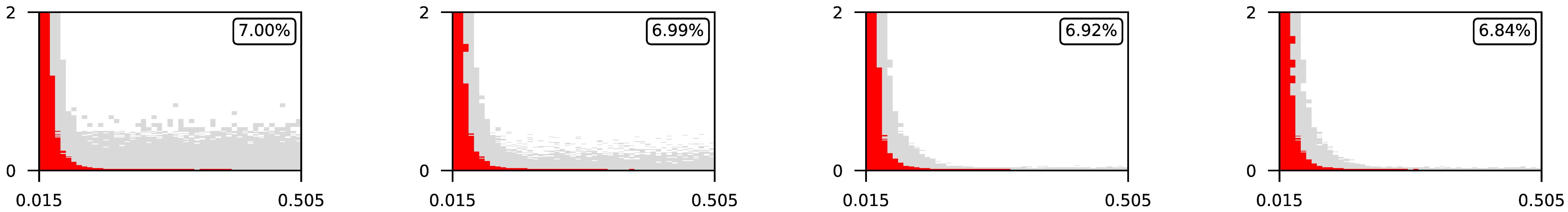 | |||
| 3 | 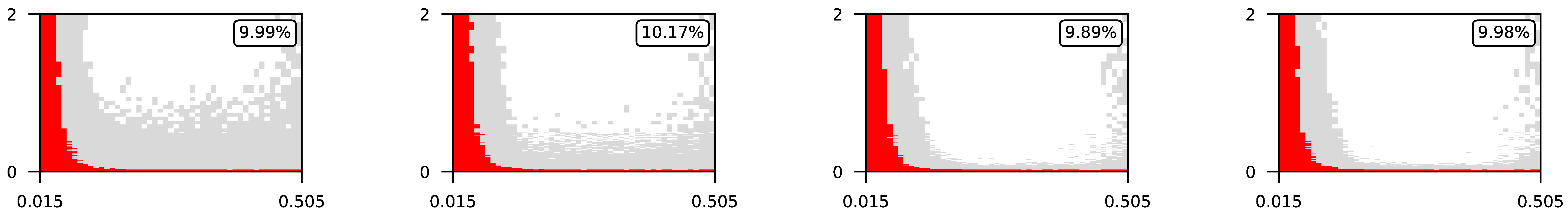 | |||
| 4 | 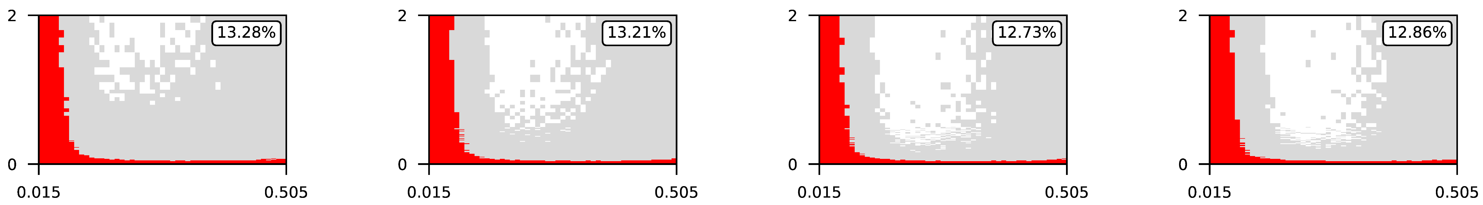 | |||
| ∖ | 0.07 | 0.1 | 0.25 | 0.5 |
|---|---|---|---|---|
| 0.5 | 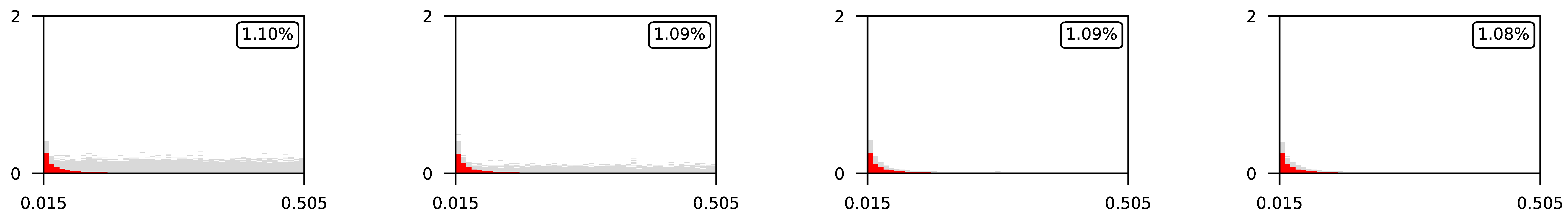 | |||
| 1 | 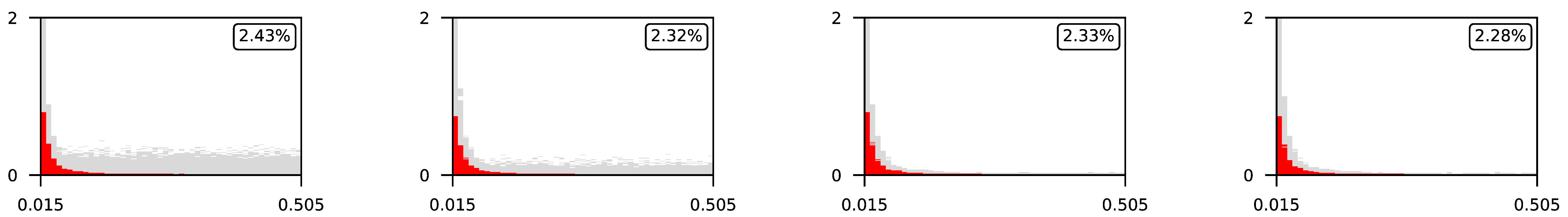 | |||
| 2 | 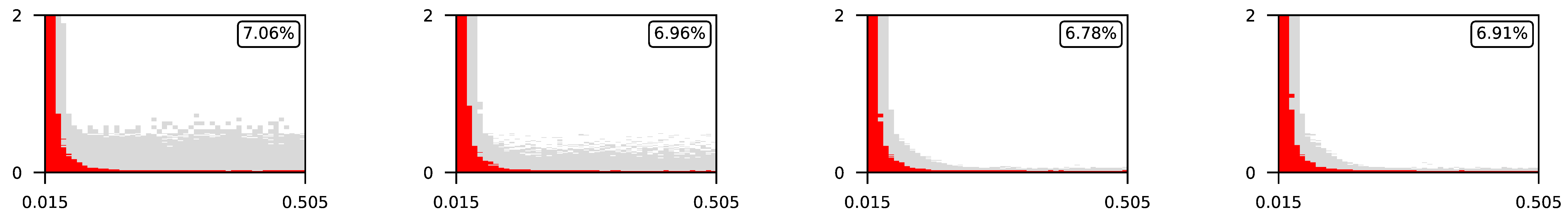 | |||
| 3 | 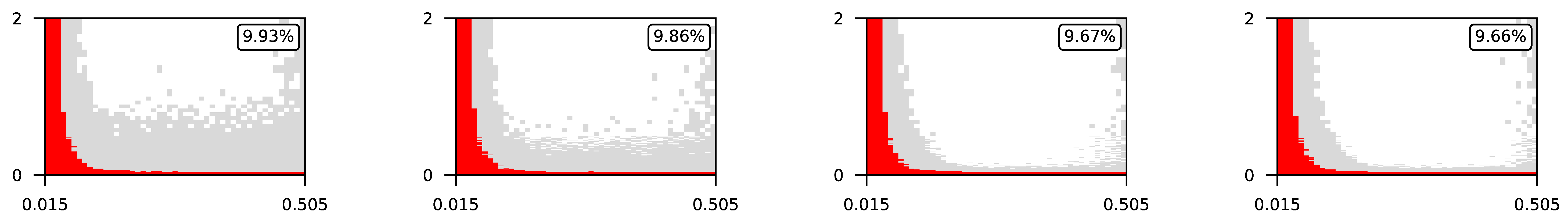 | |||
| 4 | 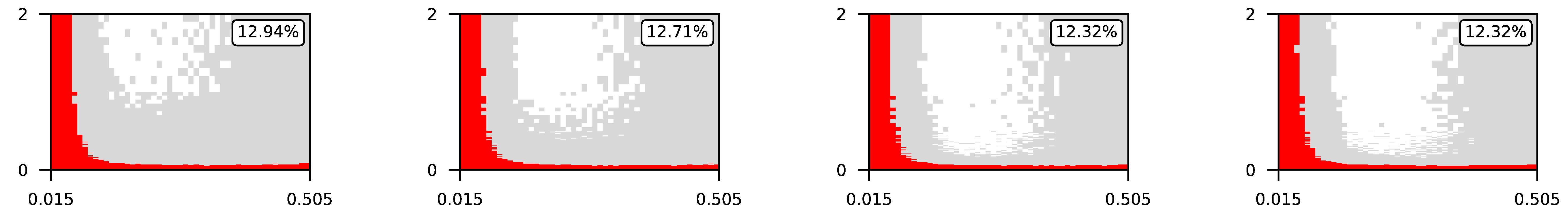 | |||
| ∖ | 0.07 | 0.1 | 0.25 | 0.5 |
|---|---|---|---|---|
| 0.5 |  | |||
| 1 |  | |||
| 2 |  | |||
| 3 | 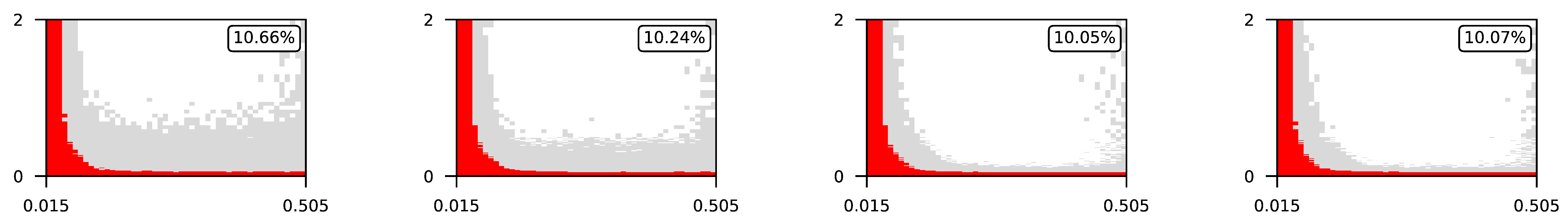 | |||
| 4 | 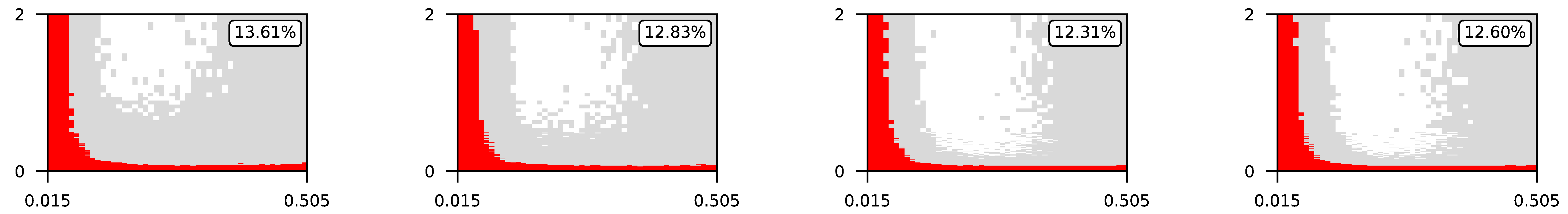 | |||
| ∖ | 0.07 | 0.1 | 0.25 | 0.5 |
|---|---|---|---|---|
| 0.5 | 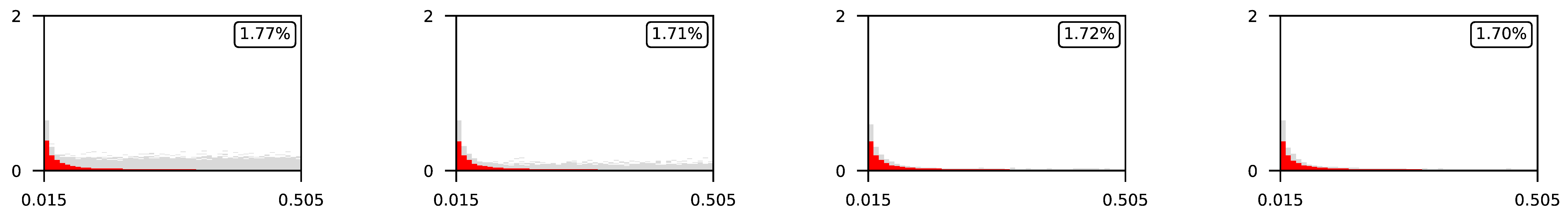 | |||
| 1 | 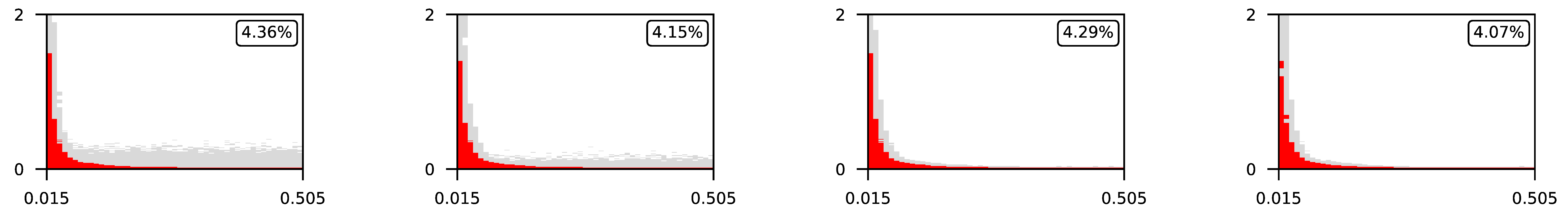 | |||
| 2 | 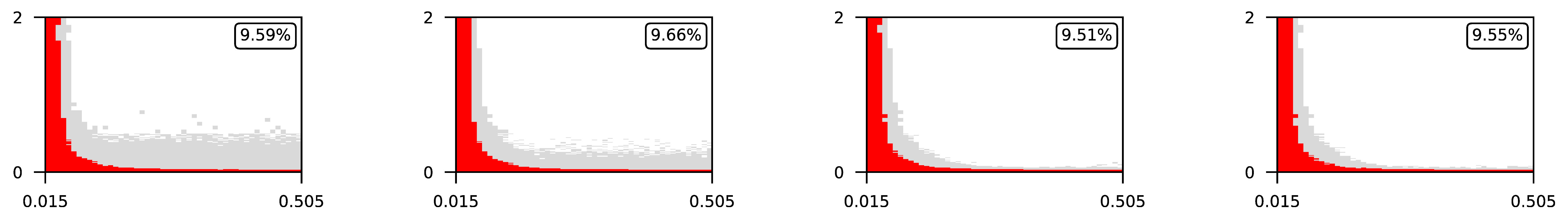 | |||
| 3 |  | |||
| 4 | 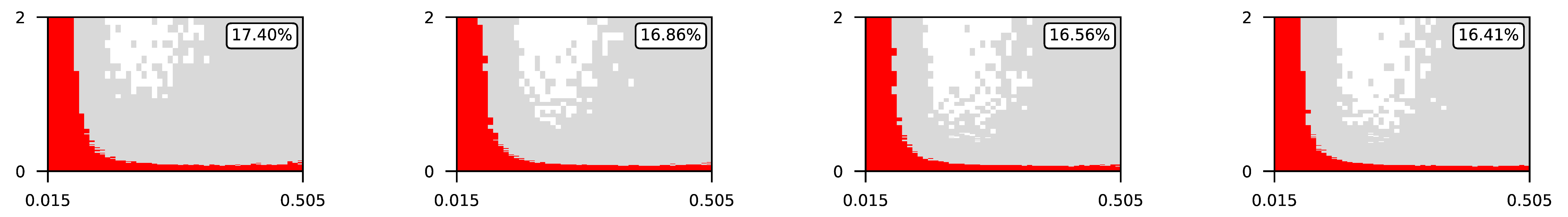 | |||
| ∖ | 0.07 | 0.1 | 0.25 | 0.5 |
|---|---|---|---|---|
| 0.5 | 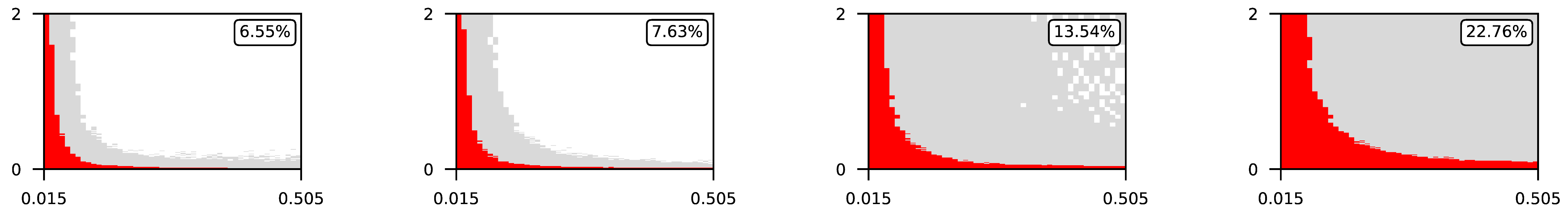 | |||
| 1 | 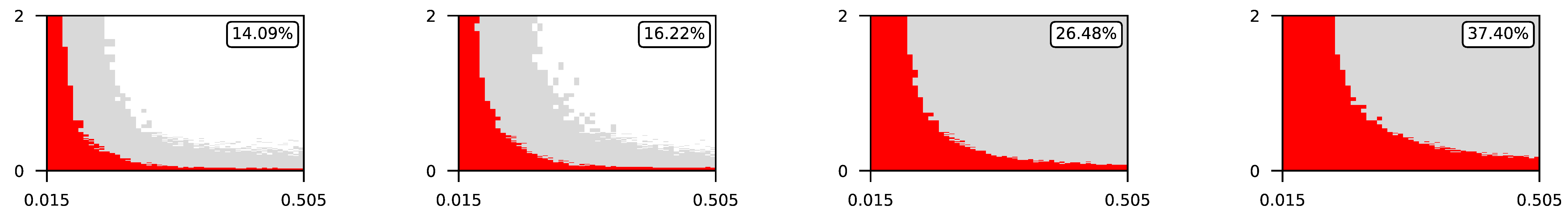 | |||
| 2 | 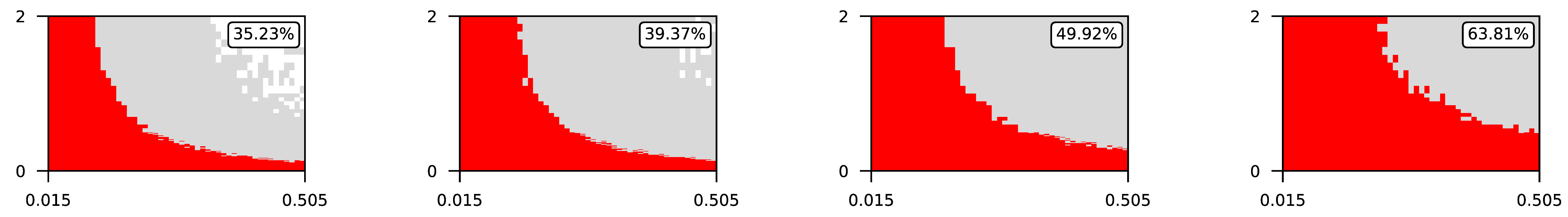 | |||
| 3 |  | |||
| 4 | 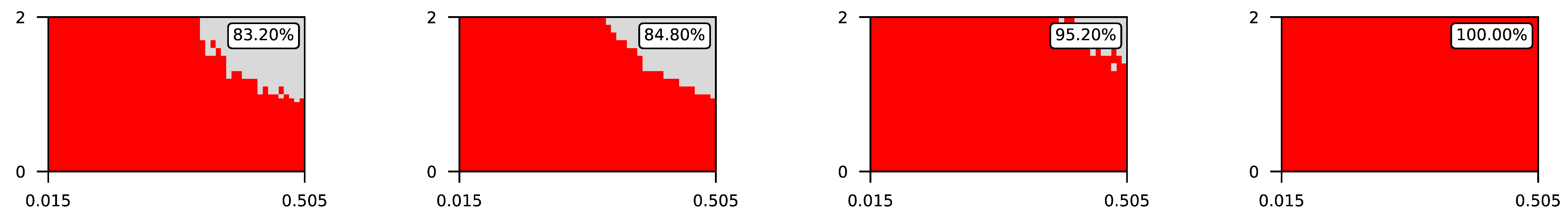 | |||
| ∖ | 0.07 | 0.1 | 0.25 | 0.5 |
|---|---|---|---|---|
| 0.5 | 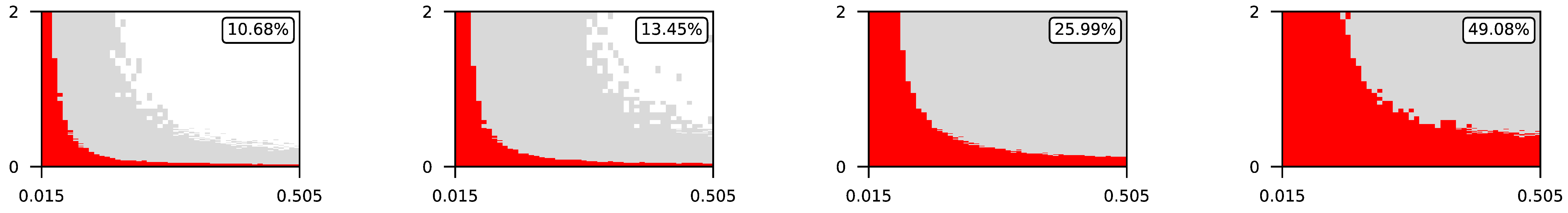 | |||
| 1 | 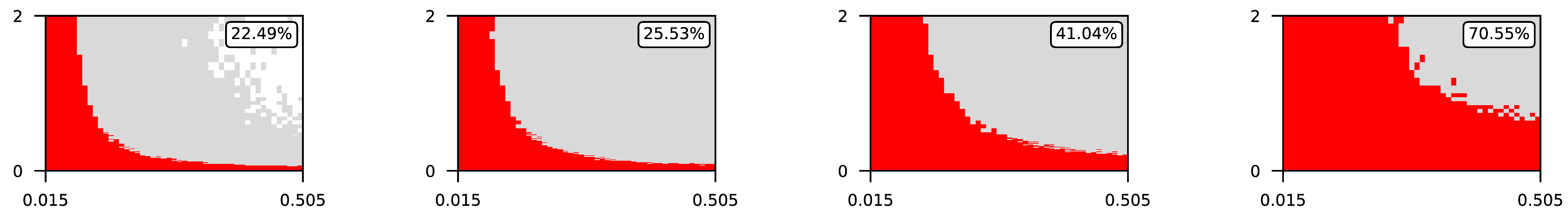 | |||
| 2 | 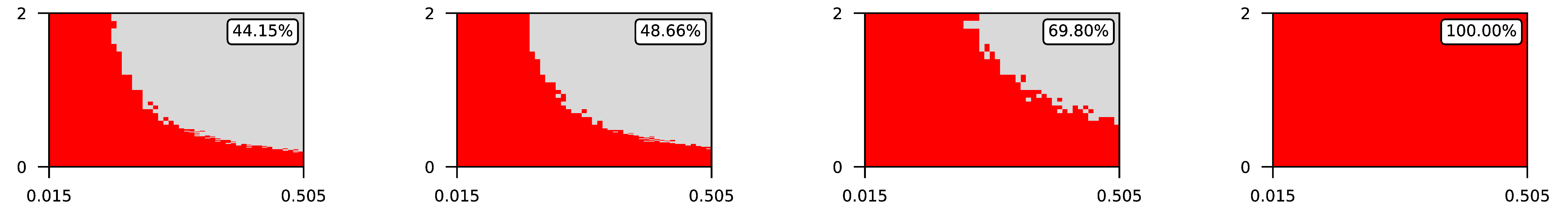 | |||
| 3 | 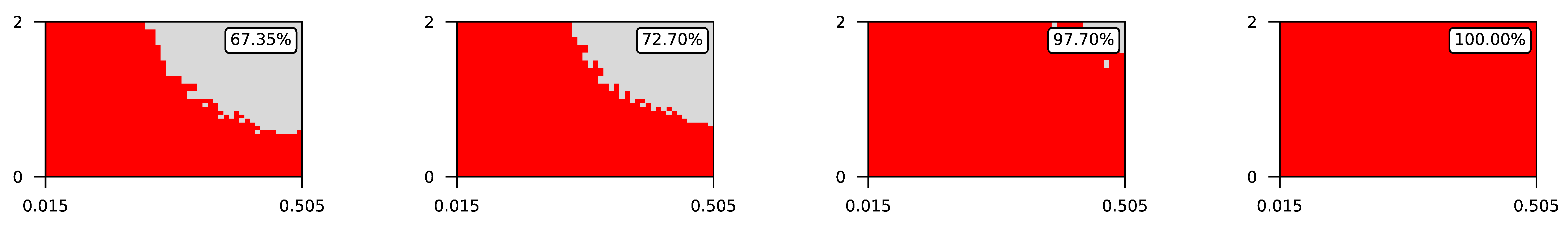 | |||
| 4 | 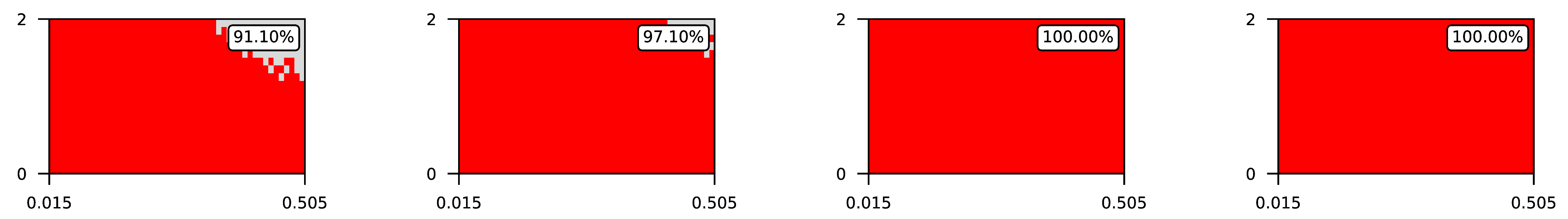 | |||
| ∖ | 0.07 | 0.1 | 0.25 | 0.5 |
|---|---|---|---|---|
| 0.5 | 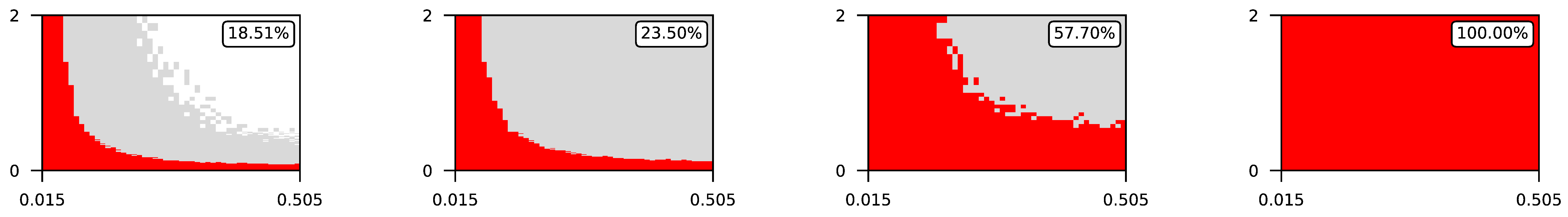 | |||
| 1 | 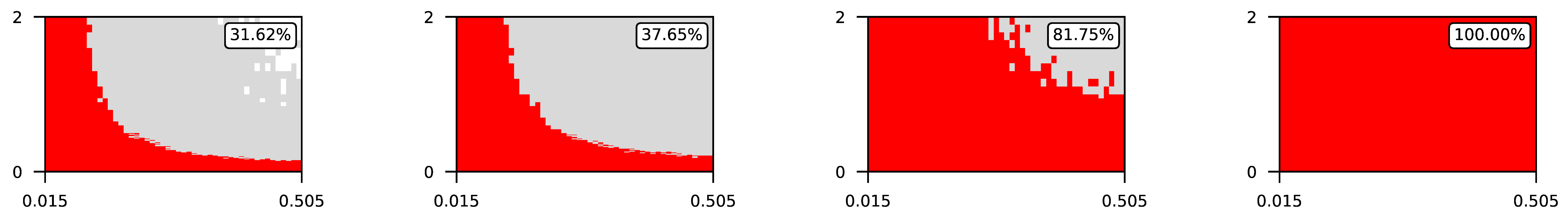 | |||
| 2 | 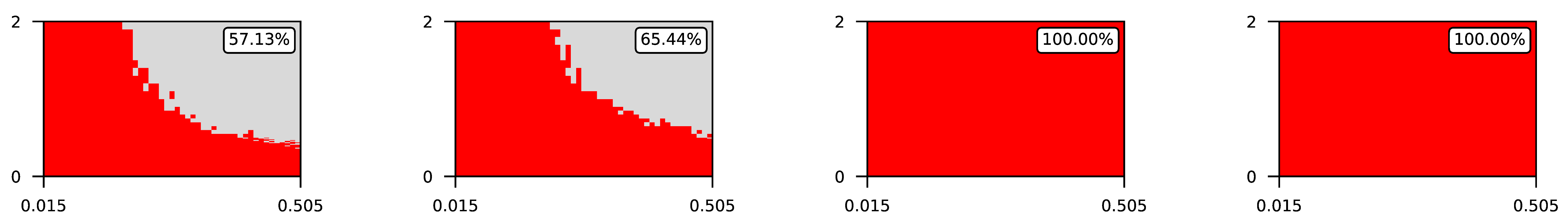 | |||
| 3 | 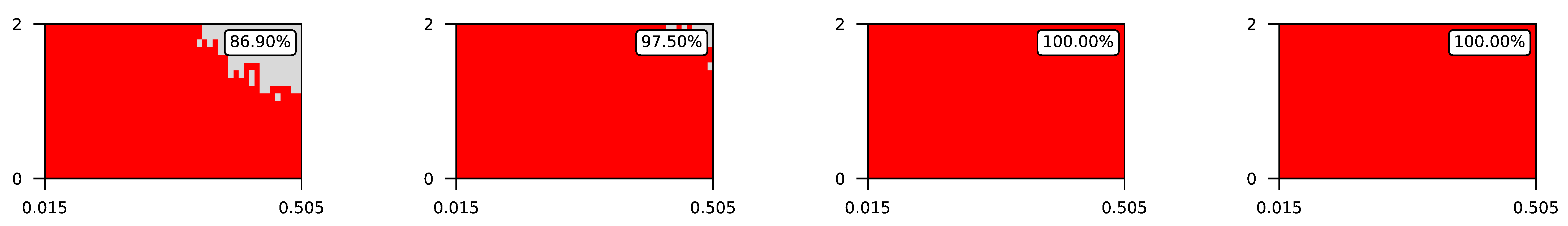 | |||
| 4 | 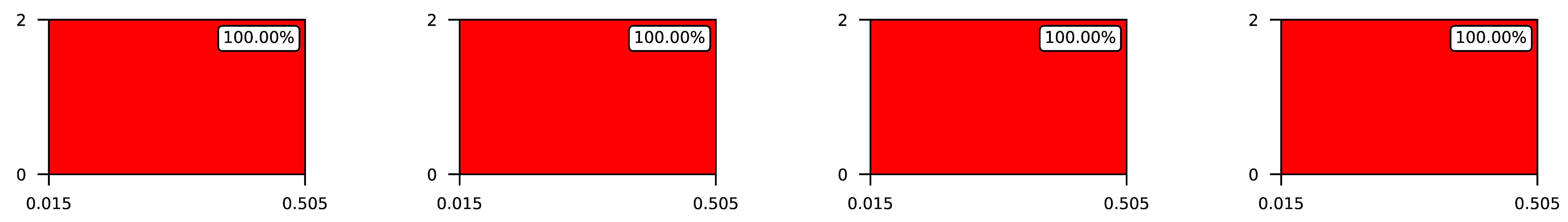 | |||
References
- Drexler, K. Engines of Creation: The Coming Era of Nanotechnology; Anchor Books; Doubleday: New York, NY, USA, 1986. [Google Scholar]
- Farazkish, R. Robust and reliable design of bio-nanorobotic systems. Microsyst. Technol. 2019, 25, 1519–1524. [Google Scholar] [CrossRef]
- Mavroidis, C.; Ferreira, A. NanoRobotics: Current Approaches and Techniques; Springer: Berlin/Heidelberg, Germany, 2012. [Google Scholar] [CrossRef]
- Decuzzi, P.; Peer, D.; Di Mascolo, D.; Palange, A.L.; Manghnani, P.N.; Moghimi, S.M.; Farhangrazi, Z.S.; Howard, K.A.; Rosenblum, D.; Liang, T.; et al. Roadmap On Nanomedicine. Nanotechnology 2020, 32, 12001–12027. [Google Scholar] [CrossRef] [PubMed]
- Webster, T. Nanomedicine: Technologies and Applications; Woodhead Publishing Series in Biomaterials; Elsevier Science: Amsterdam, The Netherlands, 2022. [Google Scholar]
- Deigner, P.; Kohl, M. Precision Medicine: Tools and Quantitative Approaches; Academic Press: Cambridge, MA, USA, 2018. [Google Scholar]
- Ginsburg, G.S. Genomic and Personalized Medicine: V1-2, 2nd ed.; ProQuest Ebook Central Leased; Elsevier Science: Saint Louis, MO, USA, 2012. [Google Scholar]
- Hao, H.; Chen, Y.F.; Wu, M. Biomimetic nanomedicine toward personalized disease theranostics. Nano Res. 2020, 14, 249–2511. [Google Scholar] [CrossRef]
- Alapan, Y.; Yasa, O.; Yigit, B.; Yasa, I.C.; Erkoc, P.; Sitti, M. Microrobotics and Microorganisms: Biohybrid Autonomous Cellular Robots. Annu. Rev. Control. Robot. Auton. Syst. 2019, 2, 205–230. [Google Scholar] [CrossRef]
- Wang, B.; Kostarelos, K.; Nelson, B.J.; Zhang, L. Trends in Micro-/Nanorobotics: Materials Development, Actuation, Localization, and System Integration for Biomedical Applications. Adv. Mater. 2021, 33, 2002047. [Google Scholar] [CrossRef]
- Holland, J.H. Hidden Order: How Adaptation Builds Complexity; Addison Wesley Longman Publishing Co., Inc.: Upper Saddle River, NJ, USA, 1996. [Google Scholar]
- Hornef, M.; Wick, M.J.; Rhen, M.; Normark, S. Bacterial strategies for overcoming host innate and adaptive immune responses. Nat. Immunol. 2002, 3, 1033–1040. [Google Scholar] [CrossRef]
- Allocati, N.; Masulli, M.; Ilio, C.D.; Laurenzi, V.D. Die for the community: An overview of programmed cell death in bacteria. Cell Death Dis. 2015, 6, e1609. [Google Scholar] [CrossRef]
- Singh, A.V.; Ansari, M.H.D.; Mahajan, M.; Srivastava, S.; Kashyap, S.; Dwivedi, P.; Pandit, V.; Katha, U. Sperm Cell Driven Microrobots—Emerging Opportunities and Challenges for Biologically Inspired Robotic Design. Micromachines 2020, 11, 448. [Google Scholar] [CrossRef]
- Wang, H.; Pumera, M. Coordinated behaviors of artificial micro/nanomachines: From mutual interactions to interactions with the environment. Chem. Soc. Rev. 2020, 49, 3211–3230. [Google Scholar] [CrossRef]
- Wang, Q.; Zhang, L. External Power-Driven Microrobotic Swarm: From Fundamental Understanding to Imaging-Guided Delivery. ACS Nano 2021, 15, 149–174. [Google Scholar] [CrossRef] [PubMed]
- Bastos-Arrieta, J.; Revilla-Guarinos, A.; Uspal, W.E.; Simmchen, J. Bacterial Biohybrid Microswimmers. Front. Robot. AI 2018, 5, 97. [Google Scholar] [CrossRef] [PubMed]
- Chen, C.; Chang, X.; Teymourian, H.; Ramirez-Herrera, D.E.; Esteban Fernandez de Avila, B.; Lu, X.; Li, J.; He, S.; Fang, C.; Liang, Y.; et al. Bioinspired Chemical Communication between Synthetic Nanomotors. Angew. Chem. Int. Ed. 2018, 57, 241–245. [Google Scholar] [CrossRef] [PubMed]
- Gao, W.; Pei, A.; Dong, R.; Wang, J. Catalytic Iridium-Based Janus Micromotors Powered by Ultralow Levels of Chemical Fuels. J. Am. Chem. Soc. 2014, 136, 2276–2279. [Google Scholar] [CrossRef] [PubMed]
- Derrien, T.L.; Hamada, S.; Zhou, M.; Smilgies, D.M.; Luo, D. Three-dimensional nanoparticle assemblies with tunable plasmonics via a layer-by-layer process. Nano Today 2020, 30, 100823. [Google Scholar] [CrossRef]
- Ma, F.; Wang, S.; Wu, D.T.; Wu, N. Electric-field–induced assembly and propulsion of chiral colloidal clusters. Proc. Natl. Acad. Sci. USA 2015, 112, 6307–6312. [Google Scholar] [CrossRef]
- Yan, J.; Han, M.; Zhang, J.; Xu, C.; Luijten, E.; Granick, S. Reconfiguring active particles by electrostatic imbalance. Nat. Mater. 2016, 15, 1095–1099. [Google Scholar] [CrossRef]
- Mou, F.; Kong, L.; Chen, C.; Chen, Z.; Xu, L.; Guan, J. Light-controlled propulsion, aggregation and separation of water-fuelled TiO2/Pt Janus submicromotors and their “on-the-fly” photocatalytic activities. Nanoscale 2016, 8, 4976–4983. [Google Scholar] [CrossRef]
- Gibbs, J.G.; Zhao, Y. Self-Organized Multiconstituent Catalytic Nanomotors. Small 2010, 6, 1656–1662. [Google Scholar] [CrossRef]
- Xie, H.; Sun, M.; Fan, X.; Lin, Z.; Chen, W.; Wang, L.; Dong, L.; He, Q. Reconfigurable magnetic microrobot swarm: Multimode transformation, locomotion, and manipulation. Sci. Robot. 2019, 4, eaav8006. [Google Scholar] [CrossRef]
- D’Souza, G.; Shitut, S.; Preussger, D.; Yousif, G.; Waschina, S.; Kost, C. Ecology and evolution of metabolic cross-feeding interactions in bacteria. Nat. Prod. Rep. 2018, 35, 455–488. [Google Scholar] [CrossRef]
- Little, A.E.; Robinson, C.J.; Peterson, S.B.; Raffa, K.F.; Handelsman, J. Rules of Engagement: Interspecies Interactions that Regulate Microbial Communities. Annu. Rev. Microbiol. 2008, 62, 375–401. [Google Scholar] [CrossRef] [PubMed]
- Moscoviz, R.; Quéméner, E.D.L.; Trably, E.; Bernet, N.; Hamelin, J. Novel Outlook in Microbial Ecology: Nonmutualistic Interspecies Electron Transfer. Trends Microbiol. 2020, 28, 245–253. [Google Scholar] [CrossRef] [PubMed]
- Russell, J. The Energy Spilling Reactions of Bacteria and Other Organisms. J. Mol. Microbiol. Biotechnol. 2007, 13, 1–11. [Google Scholar] [CrossRef] [PubMed]
- Demuth, D.; Lamont, R. Bacterial Cell-to-Cell Communication: Role in Virulence and Pathogenesis; Advances in Molecular and Cellular Microbiology; Cambridge University Press: Cambridge, UK, 2006. [Google Scholar]
- Boo, A.; Ledesma Amaro, R.; Stan, G.B. Quorum sensing in synthetic biology: A review. Curr. Opin. Syst. Biol. 2021, 28, 100378. [Google Scholar] [CrossRef]
- Rosenzweig, R.F.; Sharp, R.R.; Treves, D.S.; Adams, J. Microbial evolution in a simple unstructured environment: Genetic differentiation in Escherichia coli. Genetics 1994, 137, 903–917. [Google Scholar] [CrossRef] [PubMed]
- Pande, S.; Merker, H.; Bohl, K.; Reichelt, M.; Schuster, S.; De Figueiredo, L.; Kaleta, C.; Kost, C. Fitness and stability of obligate cross-feeding interactions that emerge upon gene loss in bacteria. ISME J. 2013, 8, 953–962. [Google Scholar] [CrossRef]
- D’Souza, G.; Kost, C. Experimental Evolution of Metabolic Dependency in Bacteria. PLoS Genet. 2016, 12, e1006364. [Google Scholar] [CrossRef]
- Varahan, S.; Laxman, S. Bend or break: How biochemically versatile molecules enable metabolic division of labor in clonal microbial communities. Genetics 2021, 219, iyab109. [Google Scholar] [CrossRef]
- Thommes, M.; Wang, T.; Zhao, Q.; Paschalidis, I.C.; Segrè, D. Designing Metabolic Division of Labor in Microbial Communities. mSystems 2019, 4, 10.1128. [Google Scholar] [CrossRef]
- Ha, P.; Lindemann, S.; Shi, L.; Dohnalkova, A.; Fredrickson, J.; Madigan, M.; Beyenal, H. Syntrophic anaerobic photosynthesis via direct interspecies electron transfer. Nat. Commun. 2017, 8, 13924. [Google Scholar] [CrossRef]
- Remis, J.P.; Wei, D.; Gorur, A.; Zemla, M.; Haraga, J.; Allen, S.; Witkowska, H.E.; Costerton, J.W.; Berleman, J.E.; Auer, M. Bacterial social networks: Structure and composition of Myxococcus xanthus outer membrane vesicle chains. Environ. Microbiol. 2014, 16, 598–610. [Google Scholar] [CrossRef] [PubMed]
- Pande, S.; Shitut, S.; Freund, L.; Westermann, M.; Bertels, F.; Colesie, C.; Bischofs, I.; Kost, C. Metabolic cross-feeding via intercellular nanotubes in bacteria. Nat. Commun. 2015, 6, 6238. [Google Scholar] [CrossRef] [PubMed]
- Mempin, R.; Tran, H.; Chen, C.; Gong, H.; Ho, K.K.; Lu, S. Release of extracellular ATP by bacteria during growth. BMC Microbiol. 2013, 13, 301. [Google Scholar] [CrossRef] [PubMed]
- Cremer, J.; Melbinger, A.; Wienand, K.; Henriquez, T.; Jung, H.; Frey, E. Cooperation in Microbial Populations: Theory and Experimental Model Systems. J. Mol. Biol. 2019, 431, 4599–4644. [Google Scholar] [CrossRef] [PubMed]
- Figueiredo, A.R.; Kümmerli, R. Microbial Mutualism: Will You Still Need Me, Will You Still Feed Me? Curr. Biol. 2020, 30, R1041–R1043. [Google Scholar] [CrossRef]
- Lopez-Garcia, P.; Moreira, D. Physical connections: Prokaryotes parasitizing their kin. Environ. Microbiol. Rep. 2020, 13, 54–61. [Google Scholar] [CrossRef]
- Pacheco, A.R.; Segrè, D. A multidimensional perspective on microbial interactions. FEMS Microbiol. Lett. 2019, 366, fnz125. [Google Scholar] [CrossRef]
- Smith, N.W.; Shorten, P.R.; Altermann, E.; Roy, N.C.; McNabb, W.C. The Classification and Evolution of Bacterial Cross-Feeding. Front. Ecol. Evol. 2019, 7, 153. [Google Scholar] [CrossRef]
- Queller, D.C.; Strassmann, J.E. Beyond society: The evolution of organismality. Philos. Trans. R. Soc. Lond. B Biol. Sci. 2009, 364, 3143–3155. [Google Scholar] [CrossRef]
- Axelrod, R. The Complexity of Cooperation: Agent-Based Models of Competition and Collaboration; Princeton University Press: Princeton, NJ, USA, 1997. [Google Scholar]
- Lindgren, K.; Nordahl, M.G. Cooperation and Community Structure in Artificial Ecosystems. Artif. Life 1993, 1, 15–37. [Google Scholar] [CrossRef]
- Kernbach, S.; Kernbach, O. Collective energy homeostasis in a large-scale microrobotic swarm. Robot. Auton. Syst. 2011, 59, 1090–1101. [Google Scholar] [CrossRef]
- Zhao, Z.; Rossiter, J. Cannibalism, altruism and trophallaxis strategies among self-sustainable swarm robots. In Proceedings of the 26th International Symposium on Artificial Life and Robotics, AROB 26th 2021, Online, 21–23 January 2021. [Google Scholar]
- Burtsev, M.; Turchin, P. Evolution of cooperative strategies from first principles. Nature 2006, 440, 1041–1044. [Google Scholar] [CrossRef] [PubMed]
- Lehmann, L.; Keller, L. The evolution of cooperation and altruism—A general framework and a classification of models. J. Evol. Biol. 2006, 19, 1365–1376. [Google Scholar] [CrossRef] [PubMed]
- Nowak, M.; Tarnita, C.; Wilson, E. The Evolution of Eusociality. Nature 2010, 466, 1057–1062. [Google Scholar] [CrossRef] [PubMed]
- Smith, J.M.; Szathmary, E. Major Transitions in Evolution; Oxford University Press: Oxford, UK, 1995. [Google Scholar]
- Wu, B.; Arranz, J.; Du, J.; Zhou, D.; Traulsen, A. Evolving synergetic interactions. J. R. Soc. Interface 2016, 13, 20160282. [Google Scholar] [CrossRef]
- André, J.B.; Nolfi, S. Evolutionary robotics simulations help explain why reciprocity is rare in nature. Sci. Rep. 2016, 6, 32785. [Google Scholar] [CrossRef]
- Floreano, D.; Mitri, S.; Perez-Uribe, A.; Keller, L. Evolution of Altruistic Robots. In Proceedings of the 2008 IEEE World Conference on Computational Intelligence: Research Frontiers, Berlin/Heidelberg, Germany, 1–6 June 2008; WCCI’08; pp. 232–248. [Google Scholar]
- Cesta, A.; Miceli, M.; Rizzo, P. Coexisting Agents: Experiments on Basic Interaction Attitude. J. Intell. Syst. 2011, 11, 1–42. [Google Scholar] [CrossRef]
- Ivanko, E. Is evolution always “egolution”: Discussion of evolutionary efficiency of altruistic energy exchange. Ecol. Complex. 2018, 34, 1–8. [Google Scholar] [CrossRef]
- Ivanko, E.E.; Chervinsky, S.M. Survival Rate of Model Populations Depending on the Strategy of Energy Exchange Between the Organisms. Izv. Saratov Univ. (N. S.) Ser. Math. Mech. Inform. 2020, 20, 241–256. (In Russian) [Google Scholar] [CrossRef]
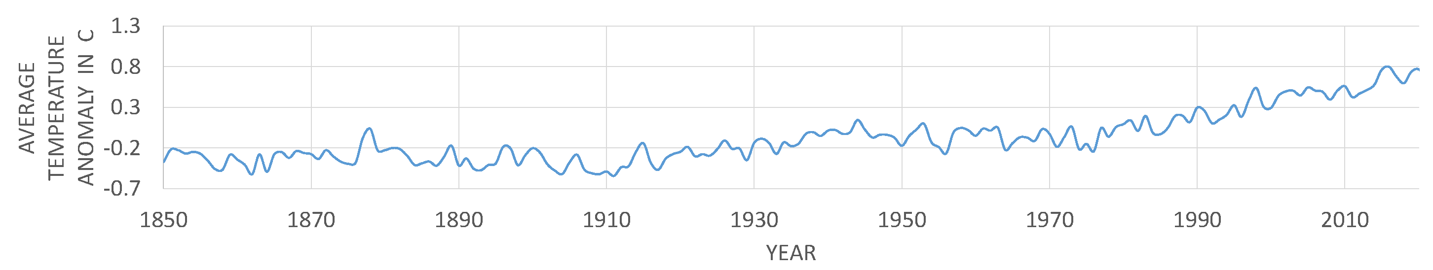
- Met Office Hadley Centre Observations Datasets. Available online: https://www.metoffice.gov.uk/hadobs/hadcrut4/data/current/time_series/HadCRUT.4.6.0.0.monthly_ns_avg.txt. (accessed on 17 October 2012).
- Krauth, J. Experimental Design: A Handbook and Dictionary for Medical and Behavioral Research; Experimental Design, Elsevier Science: Amsterdam, The Netherlands, 2000. [Google Scholar]
- Martens, A.; de Buhr, N.; Ishikawa, H.; Schroten, H.; von Köckritz-Blickwede, M. Characterization of Oxygen Levels in an Uninfected and Infected Human Blood-Cerebrospinal-Fluid-Barrier Model. Cells 2022, 11, 151. [Google Scholar] [CrossRef]
- Huus, K.E.; Ley, R.E. Blowing Hot and Cold: Body Temperature and the Microbiome. mSystems 2021, 6, 10.1128. [Google Scholar] [CrossRef] [PubMed]
- Westra, E.; Sünderhauf, D.; Landsberger, M.; Buckling, A. Mechanisms and consequences of diversity-generating immune strategies. Nat. Rev. Immunol. 2017, 17, 719–728. [Google Scholar] [CrossRef] [PubMed]

| Excluded Variable | Remained |
|---|---|
| 0.20 | |
| 0.54 | |
| 0.59 | |
| 0.49 | |
| 0.54 |
| Tree Height | 1 | 2 | 3 | 4 | 5 | |
|---|---|---|---|---|---|---|
| of full model | 0.44 | 0.57 | 0.65 | 0.70 | 0.73 | |
| without | 0.08 | 0.16 | 0.23 | 0.26 | 0.29 | |
| 0.44 | 0.56 | 0.63 | 0.68 | 0.71 | ||
| 0.44 | 0.57 | 0.69 | 0.76 | 0.81 | ||
| 0.44 | 0.54 | 0.63 | 0.67 | 0.70 | ||
| 0.44 | 0.57 | 0.65 | 0.70 | 0.73 |
Disclaimer/Publisher’s Note: The statements, opinions and data contained in all publications are solely those of the individual author(s) and contributor(s) and not of MDPI and/or the editor(s). MDPI and/or the editor(s) disclaim responsibility for any injury to people or property resulting from any ideas, methods, instructions or products referred to in the content. |
© 2024 by the authors. Licensee MDPI, Basel, Switzerland. This article is an open access article distributed under the terms and conditions of the Creative Commons Attribution (CC BY) license (https://creativecommons.org/licenses/by/4.0/).
Share and Cite
Ivanko, E.; Popel, A. Efficiency of Energy Exchange Strategies in Model Bacteriabot Populations. Micro 2024, 4, 682-705. https://doi.org/10.3390/micro4040042
Ivanko E, Popel A. Efficiency of Energy Exchange Strategies in Model Bacteriabot Populations. Micro. 2024; 4(4):682-705. https://doi.org/10.3390/micro4040042
Chicago/Turabian StyleIvanko, Evgeny, and Andrey Popel. 2024. "Efficiency of Energy Exchange Strategies in Model Bacteriabot Populations" Micro 4, no. 4: 682-705. https://doi.org/10.3390/micro4040042
APA StyleIvanko, E., & Popel, A. (2024). Efficiency of Energy Exchange Strategies in Model Bacteriabot Populations. Micro, 4(4), 682-705. https://doi.org/10.3390/micro4040042