Abstract
Immunoassays play a pivotal role in detecting and quantifying specific proteins within biological samples. However, its sensitivity and turnaround time are constrained by the passive diffusion of target molecules towards the sensors. ACET (Alternating Current Electrothermal) enhanced reaction emerges as a solution to overcome this limitation. The ACET-enhanced biosensor works by inducing vortices through electrothermal force, which stirs the analyte within the microchannel and promotes a reaction process. In this study, a comprehensive two-dimensional finite element study is conducted to optimize the binding efficiency and detection time of an ACET-enhanced biosensor without external pumping. Optimal geometries for interdigitated electrodes are estimated to achieve significant improvements in terms of probe utilization and enhancement factor. The study’s findings demonstrate enhancement factors of 3.21, 2.15, and 3.09 along with 71.22%, 75.80%, and 57.52% normalized binding for C-reactive protein (CRP), immunoglobulin (IgG), and SARS-CoV-2, respectively.
1. Introduction
Highly sensitive and rapid biosensing technologies have significant potential applications in early disease diagnosis and detection [1]. Conventional detection techniques, such as enzyme-linked immunosorbent assay (ELISA) [2] are known for their complexity and time-consuming nature. Moreover, due to slow protein-binding kinetics and inefficient mass transport in the complex liquid matrix, detecting target analyte is quite challenging, making conventional assays less suitable for rapid point-of-care testing. This is where ACEK (AC electrokinetic) enhanced biosensors demonstrate their value [3]. By combining the rapidity and simplicity derived from electrokinetic phenomena with the high affinity and specificity of probe molecules, a wide range of applications becomes feasible, particularly in point-of-care testing or lab-on-chip devices [4].
The emergence of ACEK has revolutionized the field of microfluidics by overcoming the limitations posed by direct current electrokinetics (DCEK). In contrast to DCEK, which necessitates relatively high voltages, ACEK operates at lower voltages, making it more practical for lab-on-a-chip devices [5,6]. Additionally, ACEK’s ability to produce non-uniform fluid-flow streamlines makes it valuable for fluid-mixing applications [7]. The main components of AC electrokinetics include dielectrophoresis (DEP), AC electroosmosis (ACEO), and AC electrothermal effects (ACET) [8]. By harnessing these diverse electrokinetic mechanisms, researchers have advanced fluid manipulation approaches, thereby expanding the potential of microfluidics in biomedical and analytical applications. A nonuniform AC electric field can move suspended particles through dielectrophoretic forces and induce fluid motion through the electrothermal effect or ac electro-osmosis. However, for conductive buffers, ACEO becomes invisible due to a negligible electrical double layer, resulting in no net fluid flow [9]. Conversely, at very low frequencies, ACEO might cause hydrolysis at the surface of microelectrodes [10,11]. Moreover, at the sub-micron scale, dielectrophoresis does not significantly affect particle motion [12]. An advantage of ACET over these two electrokinetic mechanisms is that it can be used for higher conductivities, i.e., over 1 S·m−1 [13]. Moreover, this technique enables the manipulation of particles ranging from bacteria to viruses (∼100 nm) and protein molecules [14,15]. While ACET-enhanced biosensors offer increased analytical sensitivity and reduced assay time, a considerable number of them necessitate intricate fluidic systems to enable continuous analyte refreshment and achieve adequate analyte binding on the sensor surface [16]. However, the precise generation of fluid flow poses a challenge for microfluidic devices [17,18]. This study aims to develop an optimized ACET-enhanced biosensor without employing external pumping, while still improving binding efficiency and significantly reducing detection time. In the following two sections, the optimization process of this ACET-enhanced biosensor will be discussed based on several binding efficiency measurement parameters.
2. Materials and Methods
2.1. ACET Flow
The AC electrothermal effect is induced when a non-uniform alternating current (AC) passes through an electrolyte [19] and induces temperature gradients in the bulk of the fluid that causes variations in permittivity and conductivity in the process. The interaction between the non-uniform AC electric fields and the gradients in conductivity and permittivity leads to ACET microflow [20]. The temperature of the fluid during steady state can be expressed by the following equation [8].
Here, T is the temperature, E is the applied electric field, k represents thermal conductivity, and σ represents the fluidic medium’s conductivity. The magnitude of the heat produced depends on the amplitude of the AC current, as well as the electrical and thermal properties of the material.
For ACET to be effective, it is important that the electric field distribution is non-uniform, and consequently, the temperature distribution within the fluid will be non-uniform (shown in Figure S1). This inhomogeneous temperature distribution will lead to temperature gradients, and in turn, temperature gradients will cause gradients in permittivity and conductivity. These gradients can be expressed by ∇ε = (∂ε/∂T)∇T and ∇σ = (∂σ/∂T)∇T. For the aqueous solution involved in this work, a linear approximation is utilized to derive the temperature dependencies of conductivity and permittivity. The permittivity and conductivity as a function of temperature can be described as ε(T) = ε(T0) + {1 + Cε(T − T0)} and σ(T) = σ(T0) + {1 + Cσ(T − T0)}. Here, T0 refers to the initial temperature of 300 K. The coefficient for conductivity, Cσ, and permittivity, Cε, can be expressed as and [21]. The resulting gradient in permittivity and conductivity induces mobile charges in the fluid bulk, according to Gauss’s law. With respect to the gradient of conductivity and permittivity, ACET force can be described by the following equation [8].
The ACET force in equation (2) consists of Coulomb force (first term of right-hand side) and dielectric force (second term of right-hand side). At lower frequencies, the Coulomb force dominates the equation whereas at higher frequencies the dielectric force dominates. The term τ = ε/σ refers to the charge relaxation time. When angular frequency ω < 1/τ, the Coulomb force dominates the dielectric force. For emulating a phosphate-buffered saline (PBS) solution having a pH of 7.2, the electrical conductivity, σ, and relative permittivity εr are set to 5.75 × 10⁻² S m−1 and 80.2, respectively [22]. The obtained electrothermal velocity is initiated as a volumetric force within the microchannel. Assuming constant viscosity, the ACET-induced flow within the microchannel can be expressed by the following equation.
Here, ρ = 100 kg.m−3 is the density of the fluid, u is velocity x-component, and v-is the velocity y-component, η = 1.08 mPa.s is the dynamic viscosity, p is the pressure.
2.2. ACET Enhanced Reaction
The analyte moves towards the reaction surface to bind with immobilized probes. The interaction between the immobilized probe and the analyte adheres to the Langmuir adsorption model of the first order [23]. ACET flow propagates the analyte A towards the sensor surface where the bio-probes B are placed and results in a binding reaction, forming an analyte–ligand complex, AB, which is a function of time. The binding reaction is dictated by analyte diffusivity, D. Both of the sided reactions in the biosensor can be expressed using the following equation.
R = ka·c·(γs − Cs) − Kd·Cs
Here, ka refers to the association constant, kd refers to the dissociation constant, γs is the active site concentration, and Cs is the bounded site concentration parameter. The reaction parameters for the experimentations are listed in Table 1.

Table 1.
Reaction parameters for different proteins [22,24].
2.3. Binding Efficiency Parameters
The binding efficiency of the proposed biosensor is examined based on three different metrics. They are as follows.
- Dimensionless Normalized Binding: Dimensionless normalized binding is an indicator of how much of the probe in the reaction channel is being utilized. Dimensionless normalized binding is measured by taking the ratio of the reaction curve at an applied voltage with respect to the active site concentration [25].
- Enhancement Factor: The enhancement factor in the context of biosensors is defined as the ratio of the initial slope of the binding reaction curve when at an applied voltage to the initial slope of the same reaction curve without applying any voltage. This factor quantifies the effect of the applied AC voltage on the binding kinetics of the analyte and ligand on the biosensor’s surface. The enhancement factor provides valuable insights into how the AC voltage influences the association and dissociation rates of the analyte–ligand interaction. A higher enhancement factor indicates that the AC voltage positively impacts the binding kinetics, leading to a more significant change in the biosensor’s response and, consequently, an improved sensitivity in detecting the target analyte [22].
- Detection Time: The detection time in the context of biosensors refers to the time it takes for the biosensor’s response to reach a certain threshold value, specifically when the surface concentration of the analyte–ligand complex reaches 95% of its maximum value. This parameter is essential as it quantifies the time required for the biosensor to detect and reach a significant level of binding between the analyte and ligand on its surface. A shorter detection time indicates that the biosensor can rapidly and efficiently detect the target analyte, making it more suitable for real-time monitoring and point-of-care testing scenarios [24].
2.4. Device Structure
An ACET-enhanced microsensor is designed with an arrangement of IDEs (interdigitated electrodes) positioned at the base of the microchannel. Figure 1 shows a cross-section of the microsensor. For a comprehensive exploration of potential electrode configurations, the setup comprises two electrodes, labeled as W1 and W2, denoting their widths. They could be equal or unequal. The gap between W1 and W2, referred to as G1, assumes a pivotal role in governing ACET-induced flow by regulating the strength of the electric field. Therefore, G1 is identified as the characteristic width according to [21]. The other gap between W2 and W1 is G2. Again, G1 and G2 could be equal or unequal. The microchannel is 200 μm thick, and filled with CRP analyte fluid. The analyte fluid in the bulk is subject to volumetric force initiated by the ACET effect. The electrodes possess a negligible thickness of 150 nm. The separation distances between the electrodes are maintained at G1 = 100 μm and G2 = 300 μm. Figure 1 shows the microsensor structure.

Figure 1.
Microchannel structure. The unoccupied regions preceding W1 and following W2 combine to create a cumulative gap, G2, with a measurement of 300 μm.
2.5. Simulation Verification
Before starting the simulation, an ACET sensor structure for CRP binding is simulated using COMSOL Multiphysics 6.1 with the same set of boundary conditions that will be applied in this work. The simulated result is found to be in good agreement with the findings from [22]. Figure S2 shows the simulated result.
3. Results
3.1. Impact of Geometrical Optimization
Optimizing the electrode’s design and experimental conditions is crucial for improving responsiveness and overall performance of ACET-enhanced biosensors. One primary approach to enhance the binding efficiency of biosensors without introducing external pumping is to increase the electrothermal force within the sample chamber. Geometric optimization plays a pivotal role in achieving this objective. By carefully designing the channel and electrode geometry, the electrothermal force can be enhanced significantly to promote a binding reaction. To underscore the impact of geometric optimization on enhancing the binding efficiency in ACET-driven reactions, we first consider a scenario where all microchannel parameters remain unchanged except for the widths of the electrodes. In the initial case, the electrode widths are 110 μm, whereas in the subsequent case, they are elongated to 200 μm. The gaps are set to 100 μm. Since the gap distances remain symmetrical, their effects negate each other. Therefore, the primary geometric factor influencing the flow of analytes inside the channel is the width of the electrode. Figure 2 illustrates that this alteration in electrode width distinctly affects the movement of analytes across the sensor surface.
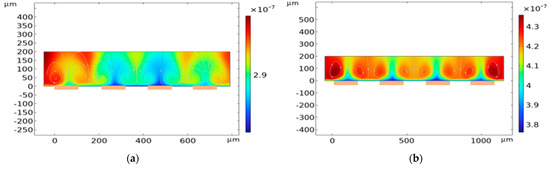
Figure 2.
Transport of analyte (concentration in mol/m−3) at the sensor surface for (a) W1 = W2 = 110 μm and (b) W1 = W2 = 200 μm. Increasing width increases electric field strength resulting in greater electrothermal velocity that causes more analytes to be distributed on top of the electrodes (locations marked in orange).
This increase in analyte distribution towards the sensor surface increases the normalized binding. Figure 3a shows the normalized binding for electrodes having a width of 100 μm to 200 μm, separated by a gap of 50 μm, 75 μm, and 100 μm. The greater binding (%) is facilitated by the enhanced flow velocity in the bulk fluid domain shown in Figure 3b. As the separation between electrodes and electrode widths are symmetrical, with respect to the increase in electrode width, the electric field components within the microchannel increase, whereas an increase in gap distance weakens the electric field strength and affects the electrothermal flow. For symmetrical configuration, the maximum normalized binding achieved is 13.1% at 50 μm gap for W1 = W2 = 200 μm. However, increasing the electrode width and reducing the gap distance to achieve greater binding is not a feasible solution in practice. Moreover, the achieved normalized binding is not optimal.
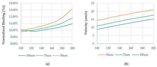
Figure 3.
For symmetrical electrode width and gap configuration, (a) normalized binding (%), and (b) velocity.
Before going through an exhaustive optimization procedure, an initial endeavor is made to enhance normalized binding by maintaining similar gaps between electrodes G1 and G2. This involves varying W1 within the range of 50 μm to 200 μm, and W2 within the range of 100 μm to 300 μm, across gap distances of 50 μm, 75 μm, and 100 μm. For these different combinations, maximum normalized binding is observed. The primary objective of this experimentation is to examine the impact of field strength in different electrode arrangements, aiming to achieve superior normalized binding compared to the results presented in Figure 3.
Figure 4 illustrates the normalized binding (%) across varying electrode setups at different gap distances. Through comprehensive simulation, the highest normalized binding percentages of 65.72%, 67.95%, and 69.66% are attained for gap distances of 50 μm, 75 μm, and 100 μm, respectively, at W2 = 300 μm and W1 = 100 μm for all the gap configurations. The average flow velocities in the bulk fluid domain are 26.14 μm/s, 20.63 μm/s, and 17.08 μm/s. Interestingly, for asymmetrical configuration at 100 μm gap, even though this recorded velocity of 17.08μm/s in the bulk is lower compared to the velocity obtained from the symmetrical configuration (21.02 μm/s), where W1 = W2 = 100 μm, and G1 = G2 = 50 μm, the achieved binding from the asymmetrical configuration is much greater.
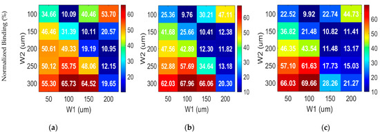
Figure 4.
Normalized binding (%) for different electrode configurations at (a) 50 μm, (b) 75 μm, and (c) 100 μm.
This phenomenon is investigated and can be explained in terms of localized velocity. Figure 5 shows localized velocity along with the streamline for Figure 5a symmetrical configuration where W1 = W2 = 200 μm and G1 = G2 = 100 μm and Figure 5b asymmetrical configuration where W1 = 125 μm, W2 = 300 μm, and G1 = G2 = 100 μm. These two configurations provide the maximum normalized binding for their respective configurations. To portray the comparison, the localized velocity is set to five different zones. For symmetrical configuration, the velocity streamline does not reach the middle portion of the electrodes and keeps propagating within the vortices. On the other hand, for asymmetrical configuration, the localized velocity in each region is greater compared to the symmetrical configuration. The velocity streamline indicates a much deeper reach towards the electrodes. Moreover, the vortices formed on top of the electrodes are pushed backward by the flow distribution formed on top of the channel which also explains the reduction in net velocity in the bulk. Due to this greater localized velocity, the normalized binding increases for asymmetrical configuration.
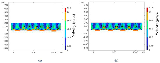
Figure 5.
Localized velocity in (μm/s) for (a) symmetrical configuration, and (b) asymmetrical configuration. The asymmetrical configuration distributes more fresh analytes from the top of the channel, resulting in greater binding reaction on top of the electrodes (locations marked in orange).
3.2. Optimization Procedure
The previous section emphasizes a crucial point—a microelectrode configuration leading to greater average bulk velocity and efficiently transports analytes across the sensor surface at an accelerated pace might not inherently maximize the binding of the analytes. Rather, it is more dependent on the localized flow and distribution of analytes along with it. This underscores the complex interplay between fluid dynamics and binding kinetics within the microchannel. It signifies that achieving optimal binding requires a delicate balance between fluid velocity and the extent of binding interactions. To maximize normalized binding through systematic geometry optimization, the critical variables of focus are W1, G1, W2, and G2. These variables are subject to constraints: W1 must be smaller than W2, and G1 must be smaller than G2. These constraints ensure the generation of directional flow. The optimization approach involves several iterative steps aimed at identifying an ideal design to maximize dimensionless normalized binding obtained from different combinations of electrode width and gap dimensions. During the optimization process, the ratios W1/G1, W2/G1, and G2/G1 are the variables under consideration. Initially, with G1 and G2 held constant, an effective width configuration is sought for W1 and W2. For the optimized electrode configurations, G2 is optimized. Subsequently, variations are introduced to G1 and the applied voltage to explore the scalability of the determined optimal electrode geometry. This iterative approach enables the systematic refinement of electrode dimensions to achieve enhanced ACET performance, facilitating the controlled manipulation of analyte flow for improved binding efficiency in the system.
3.2.1. Effective Width Configuration
To determine the most effective width configuration for the microelectrodes, the widths W1 and W2 are varied within the ranges of 50 μm to 200 μm and 100 μm to 300 μm, respectively. The gaps G1 and G2 are set to 100 μm and 300 μm, respectively. Figure 6 shows the dimensionless normalized binding (%) for these different electrode configurations at specified G1 and G2. Upon analyzing the collected data, the W1:W2 yielding the highest average bulk velocity 13.14 μm/s is 200 μm:300 μm. However, this maximum bulk velocity corresponds to a normalized binding of only 27.99% of the initial probe assigned for reaction. The optimized binding efficiency is attained under a different configuration: W1:W2 = 50 μm:250 μm, and the electrode arrangement shows 60.51% normalized binding. For W1 = 50 μm, the result shows an increase in localized velocity with respect to the increase in W2. Based on this information, the greatest amount of binding should have been achieved at a W1:W2 = 50 μm:300 μm configuration, which is not the case. This fluctuation in normalized binding and localized velocity can be explained through the concept of diffusivity.
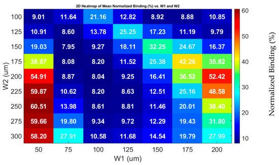
Figure 6.
Normalized binding (%) at different electrode width configurations for G1 = 100 μm and G2 = 300 μm. The maximum normalized binding 60.51% is observed at W1:W2 = 50 μm:250 μm.
A greater localized velocity indeed facilitates a faster reaction. However, if the analyte distribution happens much faster, due to the lower diffusivity of the analyte, it receives less time to react with the probed electrodes. Conversely, lower localized velocity hinders the refreshment of the sensor surface with fresh analytes. As a result, within a specific timeframe, the binding remains limited. In Figure 7a, the velocity along the length of the micro-channel is plotted for W1 = 50 μm and W2, being varied from 100 μm to 300 μm. As can be seen with respect to the increase in W2, velocity increases and a higher velocity indeed directs the analyte towards the end of the channel much faster. However, if the velocity is considerably lower the molar rate per unit area is affected adversely, which is evident for W2 = 100 μm and 150 μm shown in Figure 7b. On the other hand, if the velocity is much greater due to the lower diffusivity of the analyte, the probes placed on top of the electrode receive less time to react with the analyte, resulting in a lower molar rate per unit area. As a result, the normalized binding for W1:W2 = 50 μm:300 μm is 58.20%, which is slightly lower compared to the normalized binding of 60.51% achieved for W1:W2 = 50 μm:250 μm.
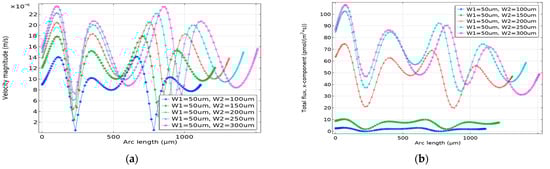
Figure 7.
(a) Velocity magnitude (m/s), and (b) molar rate per unit area per time (mol/m2.s), along (x-axis) the length of the microchannel. The molar rate is dependent on the velocity of the flow, however, for maximum binding reaction, the optimal velocity needs to be determined.
This scenario prompts further investigation to clarify the influence of localized velocity along the channel thickness. The premise is that when the analyte is driven at a significantly higher localized velocity, the analyte becomes predominantly directed toward the channel top (y-axis) before traversing across the channel. Consequently, the directional pumping along the microchannel’s length becomes less prominent, resulting in fewer analytes being bound atop the electrodes. Hence, the pumping along the length of the microchannel is less pronounced, causing fewer analytes to be bound on top of the electrodes. On the other hand, if the velocity x-component is lower along the channel thickness, the analyte on top of the microchannel is toggled less, impeding the refreshment of the sensor surface. To explain this, both x and y components of the velocity along the thickness of the microchannel are observed. The velocity y-component towards the channel thickness is shown in Figure 8a and the result shows that for W2 = 250 μm and W2 = 300 μm, the velocity y-component along the channel height is very low compared to the other W2 configurations. As a result, the effective pumping velocity of the analyte is more distributed along the x-axis for those configurations. Figure 8b shows the velocity x-component along the height of the channel. The result shows that for W2 = 250 μm the velocity x-component is greater compared to other W2 configurations, resulting in more analytes to be distributed from the top of the channel towards the sensor surface. For W2 = 250 μm and 300 μm, the vertical pumping x-component rises to 32 μm/s and 30 μm/s, respectively, and becomes less pronounced as it propagates towards the end of the micro-channel. Hence, more analytes from the top are distributed to the sensor surface.
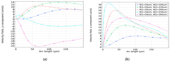
Figure 8.
Velocity magnitude (um/s) (a) y-component and (b) x-component, along the microchannel height.
3.2.2. Characteristic Length G1 Optimization
Characteristic length, G1, is optimized to examine the scalability prospect of the proposed design by maintaining the ratio between the applied voltage and characteristic length, G1. This is performed by changing the applied voltage and G1 concurrently until G1 remains above 50 μm to satisfy the fabrication resolution for the planar microelectrode design. Since the ratio between the applied voltage and G1 is 1:20 after optimizing microelectrode configuration (at 5V applied voltage and G1 = 100 μm, for optimization of W1 and W2 described in Figure 6), 3V is the minimum scaling limit that is considered in this work. The recorded average bulk velocities during these binding conditions are 14.45 μm/s at 5V, 6.18 μm/s at 4V, and 2.44 μm/s at 3V. The observed phenomenon can be attributed to the inherent relationship between voltage reduction and its consequential impact on electrothermal flow velocity, ultimately resulting in a reduction in binding efficiency. Moreover, as voltage is reduced, G2 in the optimized geometry reduces as well. For 4V and 3V, the maximum normalized binding, 54.01% and 35.04%, is achieved at G2 = 180 μm and 140 μm, respectively. The maximized normalized binding (%) along with their geometric configuration is shown in Table 2.
Table 2.
Normalized binding (%) with optimized characteristic length.
3.2.3. Optimization of G2
Since G2 shares a significant portion of the microchannel, the effectivity of the electric field influenced by W2 can be further optimized by controlling G2. Upon finding the effective width configuration for W1 and W2 of the microelectrodes and establishing a specific characteristic length, G1, the effect of G2 is further examined by varying its gap from 100 to 300 μm. The change in effective field strength in all the cases is considered by varying G1 from 50 μm to 100 μm while maintaining 5V constant. The objective is to see if the binding can be enhanced any further, as obtained from Figure 6. Table 3 shows that for an optimized electrode width configuration and specific G2, as G1 increases the average velocity in the bulk decreases. Hence, the normalized binding (%) decreases as well. With the systematic refinement, for G2 = 240 μm, 61.73% normalized binding (%) is achieved, which is greater than the normalized binding of 60.51% obtained after optimizing the microelectrode configuration W1 and W2 (in Figure 6). The normalized binding exhibits a range of values, spanning from a lower limit of 61.73% to a higher limit of 71.22% (as shown in Table 2). The G2 and G1 maintain a ratio that varies between 2.2 and 2.4, for which the observed change in normalized binding is less than 3%.
Table 3.
Normalized binding (%) at different voltages for consistent W1/G1 ratio by optimizing G2.
3.3. Enhancement Factor and Detection Time
The microchannel’s effectiveness was further evaluated in terms of binding enhancement and detection time for various protein analytes, utilizing the reaction parameters outlined in Table 1. The simulation is performed for 50 minutes, yielding maximum binding percentages of 71.22% for CRP, 75.80% for IgG, and 57.52% for SARS-COV-2. Notably, both the normalized binding and enhancement factors are almost comparable to findings reported in references [22] and [24], despite slightly prolonged detection times for CRP and IgG. It is imperative to note that in this study, the applied voltage is limited to 5V, in contrast to the 15V utilized in the ACET simulation in [22], a choice made to mitigate electrolysis and electrode degradation in practical applications. Furthermore, our proposed sensing system exhibited favorable detection times in all the cases, especially for SARS-COV-2. Detailed binding efficiency parameters for various proteins are presented in Table 4.
Table 4.
Binding efficiency parameters for different proteins over 50 min.
4. Discussion
The proposed microchannel design provides a lot of promising features. The optimized geometry does not require excessive extension of electrode widths for enhanced field strength to promote ACET. Hence, these width-optimized biosensors are more favorable for lab-on-chip applications and can be integrated into handheld devices for rapid and accurate diagnosis of diseases due to their compact size and significantly faster response time. Furthermore, no additional external pumping is required to refresh the sensor surface as depicted both in [22,24]. From the replicated result of [22], the normalized binding (%) for CRP complex is slightly less than 85%, with an association enhancement factor of 5.17 and detection time of 240s achieved at 15 V. However, in practical applications 15 V is a very large voltage for generating ACET flow and might cause electrolysis of the electrode within its detection time range, affecting the binding reaction by deteriorating the electrodes and probes, and causing electrolytic decomposition. Moreover, the gap G1 in the geometry is 15um, which might make the fabrication process challenging and quite expensive for lab-on-chip applications [26,27,28]. Moreover, 50 μm is a considerable design margin since it can be achieved easily in planar designs [29]. For the proposed geometry, both the normalized binding and enhancement factor fall within a satisfactory margin without the necessity of any external pumping, even though the detection time is significantly greater.
5. Conclusions
The proposed microchannel design offers significant advantages by circumventing the need for electrode width extensions and external pumping. Despite practical voltage constraints and fabrication intricacies, it promises favorable binding and enhancement outcomes suitable for diverse applications, including healthcare, environmental monitoring, lab-on-chip devices, and handheld diagnostics. This study not only enhances the capabilities of tiring immunoassays but also opens up the door to quicker and more cost-effective healthcare solutions in the long run.
Supplementary Materials
The following supporting information can be downloaded at: https://www.mdpi.com/article/10.3390/micro3040054/s1, Figure S1: Electric Potential, Temperature and Velocity Distribution; Figure S2: Simulation Verification.
Author Contributions
Conceptualization, J.W.; methodology, S.I. and J.W.; software, S.I.; investigation, S.I. and J.W; resources, J.W.; data curation, S.I.; writing—original draft preparation, S.I.; writing—review and editing, S.I. and J.W; supervision, J.W.; project administration, J.W.; funding acquisition, J.W. All authors have read and agreed to the published version of the manuscript.
Funding
This research was funded by Tennessee Institute for a Secure & Sustainable Environment.
Institutional Review Board Statement
Not applicable.
Informed Consent Statement
Not applicable.
Data Availability Statement
The data that support the findings of this study are available from the authors upon request.
Conflicts of Interest
The authors declare no conflict of interest.
References
- An, J.; Ding, S.; Hu, X.; Sun, L.; Gu, Y.; Xu, Y.; Hu, Y.; Liu, C.; Zhang, X. Preparation, characterization and application of anti-human OX40 ligand (OX40L) monoclonal antibodies and establishment of a sandwich ELISA for autoimmune diseases detection. Int. Immunopharmacol. 2019, 67, 260–267. [Google Scholar] [CrossRef] [PubMed]
- Alhajj, M.; Zubair, M.; Farhana, A. Enzyme Linked Immunosorbent Assay. In StatPearls; StatPearls Publishing: Treasure Island, FL, USA, 2023. Available online: http://www.ncbi.nlm.nih.gov/books/NBK555922/ (accessed on 10 August 2023).
- Song, M.; Lin, X.; Peng, Z.; Zhang, M.; Wu, J. Enhancing affinity-based electroanalytical biosensors by integrated AC electrokinetic enrichment—A mini review. Electrophoresis 2022, 43, 201–211. [Google Scholar] [CrossRef] [PubMed]
- Li, D. Electrokinetics in Microfluidics; Interface Science and Technology Series, no. 2. Elsevier-Academic Press: Amsterdam, The Netherlands; Boston, MA, USA; Heidelberg, Germany, 2004. [Google Scholar]
- Sigurdson, M.; Wang, D.; Meinhart, C.D. Electrothermal stirring for heterogeneous immunoassays. Lab Chip 2005, 5, 1366. [Google Scholar] [CrossRef]
- Lian, M.; Islam, N.; Wu, J. AC electrothermal manipulation of conductive fluids and particles for lab-chip applications. IET Nanobiotechnol. 2007, 1, 36. [Google Scholar] [CrossRef]
- Lian, M.; Wu, J. Ultrafast micropumping by biased alternating current electrokinetics. Appl. Phys. Lett. 2009, 94, 064101. [Google Scholar] [CrossRef]
- Ramos, A.; Morgan, H.; Green, N.G.; Castellanos, A. Ac electrokinetics: A review of forces in microelectrode structures. J. Phys. Appl. Phys. 1998, 31, 2338–2353. [Google Scholar] [CrossRef]
- Green, N.G.; Ramos, A.; González, A.; Morgan, H.; Castellanos, A. Fluid flow induced by nonuniform ac electric fields in electrolytes on microelectrodes. I. Experimental measurements. Phys. Rev. E 2000, 61, 4011–4018. [Google Scholar] [CrossRef]
- Wu, J. Biased AC electro-osmosis for on-chip bioparticle processing. IEEE Trans. Nanotechnol. 2006, 5, 84–89. [Google Scholar] [CrossRef]
- Wu, J.J. Ac electro-osmotic micropump by asymmetric electrode polarization. J. Appl. Phys. 2008, 103, 024907. [Google Scholar] [CrossRef]
- Pethig, R. Review Article—Dielectrophoresis: Status of the theory, technology, and applications. Biomicrofluidics 2010, 4, 022811. [Google Scholar] [CrossRef]
- Morgan, H.; Green, N.G. AC Electrokinetics: Colloids and Nanoparticles; Microtechnologies and Microsystems Series, no. 2; Research Studies Press: Baldock, UK, 2003. [Google Scholar]
- Wang, X.-B.; Huang, Y.; Gascoyne, P.; Becker, F. Dielectrophoretic manipulation of particles. IEEE Trans. Ind. Appl. 1997, 33, 660–669. [Google Scholar] [CrossRef]
- Morgan, H.; Hughes, M.P.; Green, N.G. Separation of Submicron Bioparticles by Dielectrophoresis. Biophys. J. 1999, 77, 516–525. [Google Scholar] [CrossRef] [PubMed]
- Li, J.; Lillehoj, P.B. Ultrafast Electrothermal Flow-Enhanced Magneto Biosensor for Highly Sensitive Protein Detection in Whole Blood. Angew. Chem. Int. Ed. 2022, 61, e202200206. [Google Scholar] [CrossRef] [PubMed]
- Zhao, C.; Yang, C. Advances in electrokinetics and their applications in micro/nano fluidics. Microfluid. Nanofluidics 2012, 13, 179–203. [Google Scholar] [CrossRef]
- Wu, J.; Lian, M.; Yang, K. Micropumping of biofluids by alternating current electrothermal effects. Appl. Phys. Lett. 2007, 90, 234103. [Google Scholar] [CrossRef]
- AKoklu, A.; El Helou, A.; Raad, P.E.; Beskok, A. Characterization of Temperature Rise in Alternating Current Electrothermal Flow Using Thermoreflectance Method. Anal. Chem. 2019, 91, 12492–12500. [Google Scholar] [CrossRef]
- Lijnse, T.; Cenaiko, S.; Dalton, C. Numerical simulation of a tuneable reversible flow design for practical ACET devices. SN Appl. Sci. 2020, 2, 305. [Google Scholar] [CrossRef]
- Yuan, Q.; Yang, K.; Wu, J. Optimization of planar interdigitated microelectrode array for biofluid transport by AC electrothermal effect. Microfluid. Nanofluidics 2014, 16, 167–178. [Google Scholar] [CrossRef]
- Huang, K.-R.; Chang, J.-S.; Chao, S.D.; Wu, K.-C.; Yang, C.-K.; Lai, C.-Y.; Chen, S.-H. Simulation on binding efficiency of immunoassay for a biosensor with applying electrothermal effect. J. Appl. Phys. 2008, 104, 064702. [Google Scholar] [CrossRef]
- Camillone, N. Diffusion-Limited Thiol Adsorption on the Gold(111) Surface. Langmuir 2004, 20, 1199–1206. [Google Scholar] [CrossRef]
- Kaziz, S.; Saad, Y.; Gazzah, M.H.; Belmabrouk, H. 3D simulation of microfluidic biosensor for SARS-CoV-2 S protein binding kinetics using new reaction surface design. Eur. Phys. J. Plus 2022, 137, 241. [Google Scholar] [CrossRef] [PubMed]
- Sigurdson, M.; Meinhart, C.; Liu, X.; Wang, D. Biosensor Performance Enhancement through Ac Electrokinetics. 2003. Available online: https://www.semanticscholar.org/paper/BIOSENSOR-PERFORMANCE-ENHANCEMENT-THROUGH-AC-Sigurdson-Meinhart/8d12eff79b1f9cc81cecfb3158c4e9dad10e15c5 (accessed on 11 August 2023).
- Ng, W.Y.; Goh, S.; Lam, Y.C.; Yang, C.; Rodríguez, I. DC-biased AC-electroosmotic and AC-electrothermal flow mixing in microchannels. Lab Chip 2009, 9, 802–809. [Google Scholar] [CrossRef] [PubMed]
- Wilber, H.W. Alternating Current Electrolysis with Zinc Electrodes in Sodium Thiosulphate Solution; Rice University: Houston, TX, USA, 1917. [Google Scholar]
- Tibbe, M.; Loessberg-Zahl, J.; Do Carmo, M.P.; van der Helm, M.; Bomer, J.; Van Den Berg, A.; Le-The, H.; Segerink, L.; Eijkel, J. Large-scale fabrication of free-standing and sub-μm PDMS through-hole membranes. Nanoscale 2018, 10, 7711–7718. [Google Scholar] [CrossRef]
- How to Choose the Most Appropriate Technology: FDM, SLA and SLS. Available online: https://filament2print.com/gb/blog/92_3d-printing-fdm-sla-sls-technology.html (accessed on 11 August 2023).
Disclaimer/Publisher’s Note: The statements, opinions and data contained in all publications are solely those of the individual author(s) and contributor(s) and not of MDPI and/or the editor(s). MDPI and/or the editor(s) disclaim responsibility for any injury to people or property resulting from any ideas, methods, instructions or products referred to in the content. |
© 2023 by the authors. Licensee MDPI, Basel, Switzerland. This article is an open access article distributed under the terms and conditions of the Creative Commons Attribution (CC BY) license (https://creativecommons.org/licenses/by/4.0/).