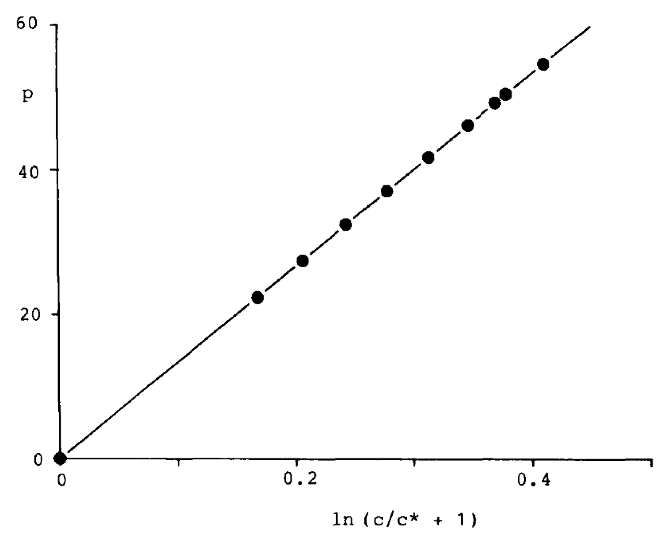
Figure 1.
Typical linear correlation between p and ln (c/c* + 1) according to Equation (5): CO2 at 75.260 °C, c < 3.1 mol·L−1; E = 133.4 at, c* = 4.5 mol·L−1, r = 0.999 998, n = 10; deviations in the correlation from experimental data of 10 until 20 ppm.
Figure 1.
Typical linear correlation between p and ln (c/c* + 1) according to Equation (5): CO2 at 75.260 °C, c < 3.1 mol·L−1; E = 133.4 at, c* = 4.5 mol·L−1, r = 0.999 998, n = 10; deviations in the correlation from experimental data of 10 until 20 ppm.
Figure 2.
Diagram of state of CO
2: Discontinuous measurements were taken from Refs. [
6,
7,
8], and curves were calculated [
5] by means of Equations (5) and (8) and the application of the method of least squares to fit the experimental data. Measurements at very high pressure were included, but not shown in the right-hand diagram for graphical clarity. Temperatures (rounded): 25, 32, 40, 50, 75, 100, and 140 °C (see Ref. [
9])
ck(I-II) ≅ 3.1 mol·L
−1 (concentration for the change from solvent structure I to II),
ck(II-III) ≅ 10 mol·L
−1 (concentration for the change from solvent structure II to III). (
a) Enlarged region I (
c < 3.1 mol·L
−1). (
b) Complete region I, II, and III; filled circles for region I and III, squares for region II, triangles for the biphasic region.
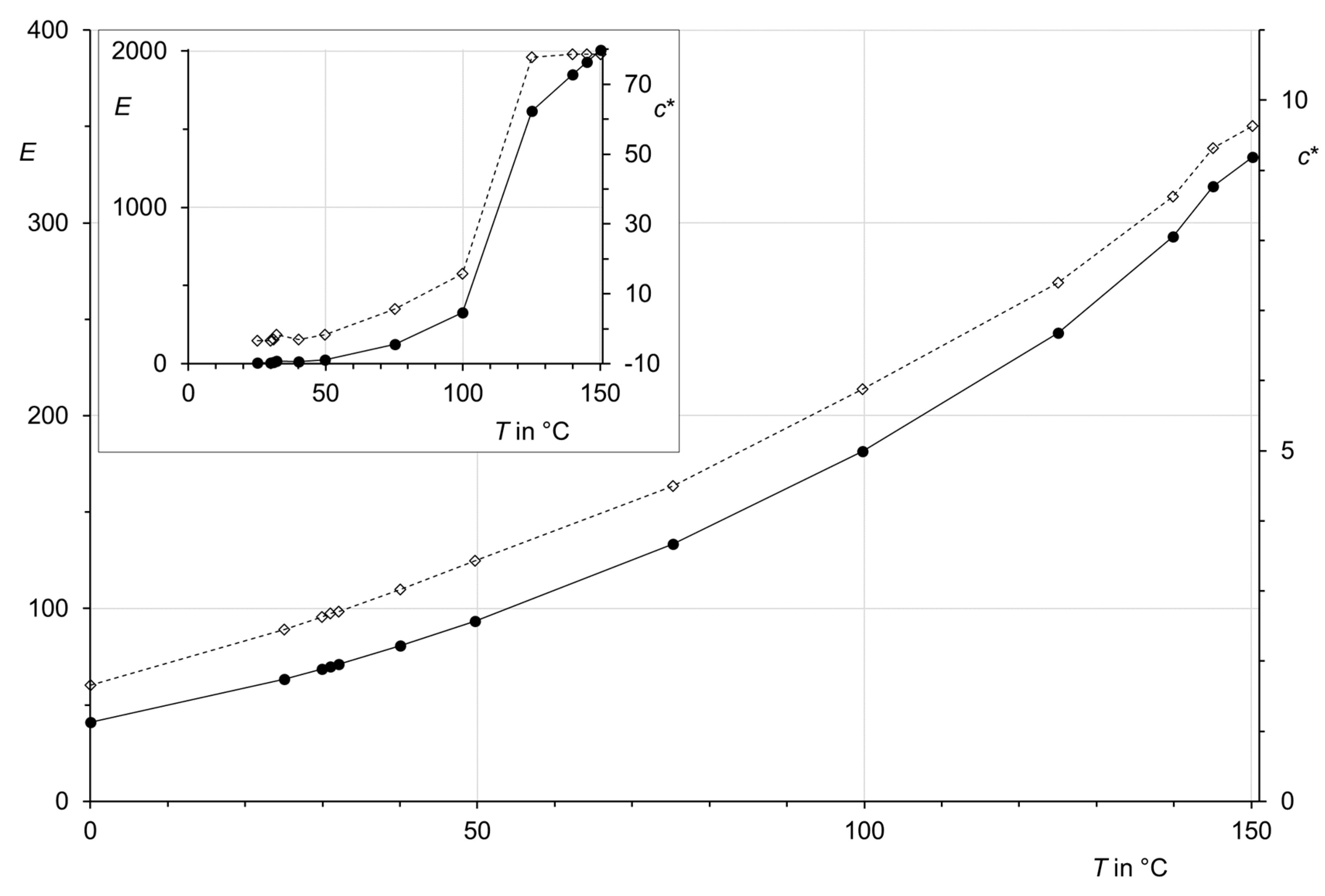
Figure 3.
Temperature dependence (T) of the parameters E (solid curve and filled circles) and c* (dashed curves and open diamonds) of Equation (5) for CO2 and region I. Inset: parameters for region II.
Figure 3.
Temperature dependence (T) of the parameters E (solid curve and filled circles) and c* (dashed curves and open diamonds) of Equation (5) for CO2 and region I. Inset: parameters for region II.
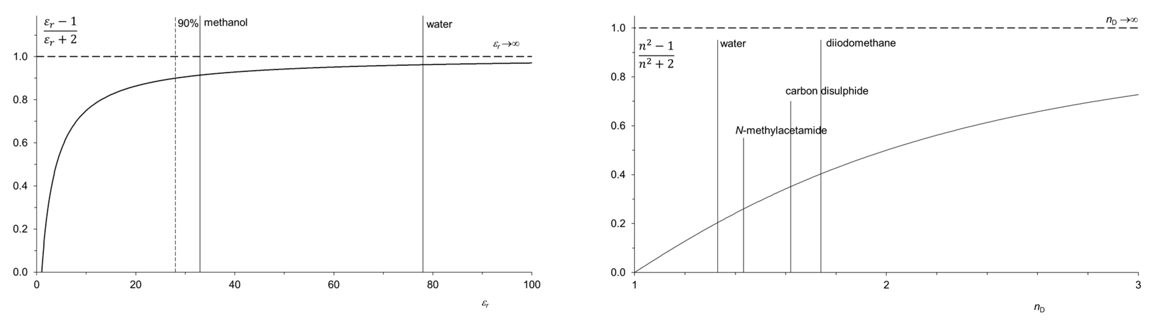
Figure 4.
(
Left) Kirkwood function (vertical axis) as a function of the relative dielectric permittivity
εr. The dashed vertical line corresponds to 90% of the maximal value of the Kirkwood function [
22]. The
εr values of methanol (33) and water (78) are indicated by vertical lines. (
Right) The index of refraction
nD as a measure of the polarizability of solvents. The region of
nD of solvents essential for preparative chemistry extends between the values for water (1.33) and diiodomethane (1.74). The values of the highly polarizable carbon disulfide (1.62) as versatile solvent and
N-methylacetamide (1.43) with high
εr are marked by vertical lines.
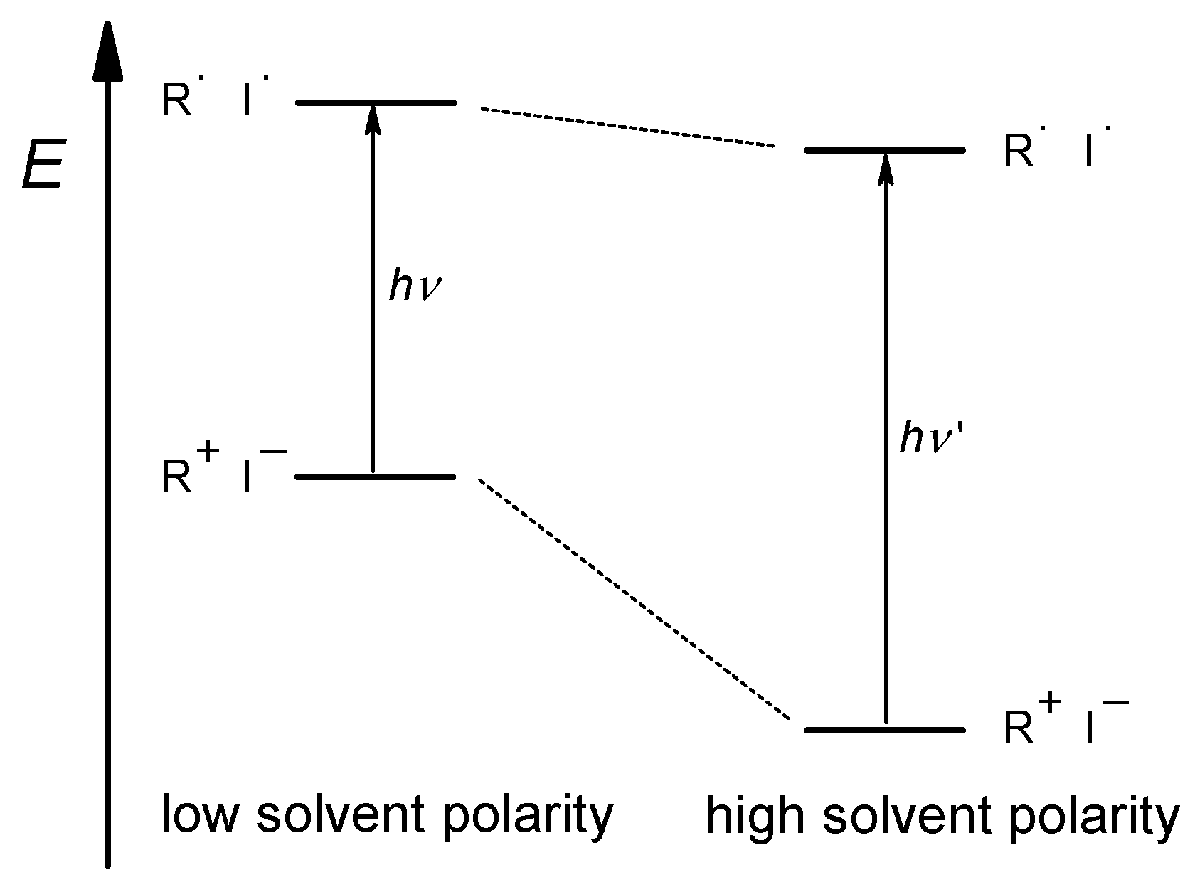
Figure 5.
Schematic representation of the solvent effect on the energetic position (E) of dye 2 in the electronic ground and excited states: The energy difference is related to the wavelengths λ of the absorbed light in the CT transition ΔE = hν = h·c/λ.
Figure 5.
Schematic representation of the solvent effect on the energetic position (E) of dye 2 in the electronic ground and excited states: The energy difference is related to the wavelengths λ of the absorbed light in the CT transition ΔE = hν = h·c/λ.
Figure 6.
Linear correlation (diamonds) for solvent effects (LFE) between the Y scale (t-BuCl 1) and the ET(30) scale (compound 3, right ordinate, correlation number 0.97 with 5 solvents, coefficient of determination 0.94, standard deviation 0.66, slope 0.46, intercept –26; solvents from right to left: H2O, HCONH2, CH3CO2H, CH3OH, C2H5OH). Linear correlation for the Z scale (compound 2) and the ET(30) scale (compound 3, left ordinate, correlation number 0.995 for 18 solvents, coefficient of determination 0.991, standard deviation 1.0, slope 1.33, intercept 11.0; solvents from right to left: (hydrogen-bonding solvents: hollow circles) H2O, HOCH2CH2OH, CH3OH, C2H5OH, 2-C3H7OH, n-C4H9-1-OH, 1-C3H7OH; (non-hydrogen-bonding solvents: Filled circles) CH3CN, DMSO, t-C4H9OH, DMF, (CH3)2CO, CH2Cl2, pyridine, CHCl3, CH3OCH2CH2OCH3, THF, 1,4-dioxane. Inset: Linear correlation between the Y scale (t-C4H9Cl 1) and the Z scale (compound 2, correlation number 0.96 for 5 solvents, coefficient of determination 0.91, standard deviation 2.1, slope 2.6, intercept 84; solvents from right to left: H2O, HCONH2, CH3CO2H, CH3OH, C2H5OH).

Figure 7.
Linear correlation between the
ET(30) (dye
3) and
ET(26) (dye
4) values for pure solvents from Ref. [
47] the standard deviations are indicated. Filled circles and solid line: non-hydrogen-bonding solvents; slope: 0.64; intercept: 11.5 correlation number 0.993 for 15 solvents, standard deviation 0.30; coefficient of determination 0.987. Open circles and dashed line: Hydrogen-bonding solvents; slope: 1.1; intercept: −12.1; correlation number 0.960 for 13 solvents; standard deviation 1.31; coefficient of determination 0.924. Solvents with increasing
ET(30) values: C
6H
5CH
3, C
6H
6, C
6H
5OC
6H
5, 1,4-dioxane, 2,6-lutidine, (CH
2)
4O, C
6H
5Cl, CH
3OCH
2CH
2OCH
3, CHCl
3, C
5H
5N, CH
2Cl
2, CH
3COCH
3, HCON((CH
3)
2, (CH
3)
3COH, C
6H
5NH
2, CH
3SOCH
3, CH
3CN, (CH
3)
2CHCH
2CH
2OH, 2,6-(CH
3)
2C
6H
3OH, CH
3CHOHCH
3, CH
3CH
2CH
2CH
2OH, CH
3CH
2CH
2OH, C
6H
5CH
2OH, CH
3CH
2OH, HOCH
2CH
2OCH
3, HCONHCH
3, CH
3OH, HOCH
2CH
2OH.
Figure 8.
Linear correlation of polarity scales for the pure solvents water (1), methanol (2), ethanol (3), dimethylformamide (DMF, 4), dimethylphthalate (5), butyronitrile (6), acetonitrile (7), acetone (8), chloroform (9), diethylphthalate (10), tetrahydrofurane (THF, 11), ethylacetate (12), 1,4-dioxane (13), dichloromethane (14), dimethylsulfoxide (DMSO, 15), bromobenzene (16), chlorobenzene (17), m-xylene (18), toluene (19), formamide (20), and pyridine (21). (a) Molar energy of the fluorescence of 10 (∑ scale) versus the ET(30) scale; (b) molar energy of the optical excitation of 10 (σ scale) versus the χR scale. The larger scattering of points compared to previous plots is attributed to some contributions of specific solvent interactions.
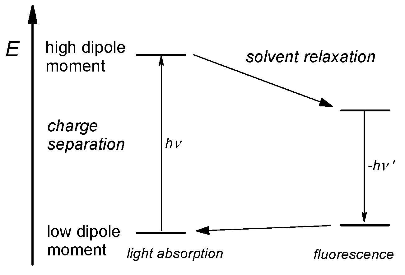
Figure 9.
Schematic representation of the solvent effect on the energetic position (E) of dye 10 in the electronic ground and excited state (ΔE = hν = h·c/λ). The electronic excitation of 10 causes a charge separation, with subsequent solvent relaxation affecting the wavelength of fluorescence.
Figure 9.
Schematic representation of the solvent effect on the energetic position (E) of dye 10 in the electronic ground and excited state (ΔE = hν = h·c/λ). The electronic excitation of 10 causes a charge separation, with subsequent solvent relaxation affecting the wavelength of fluorescence.
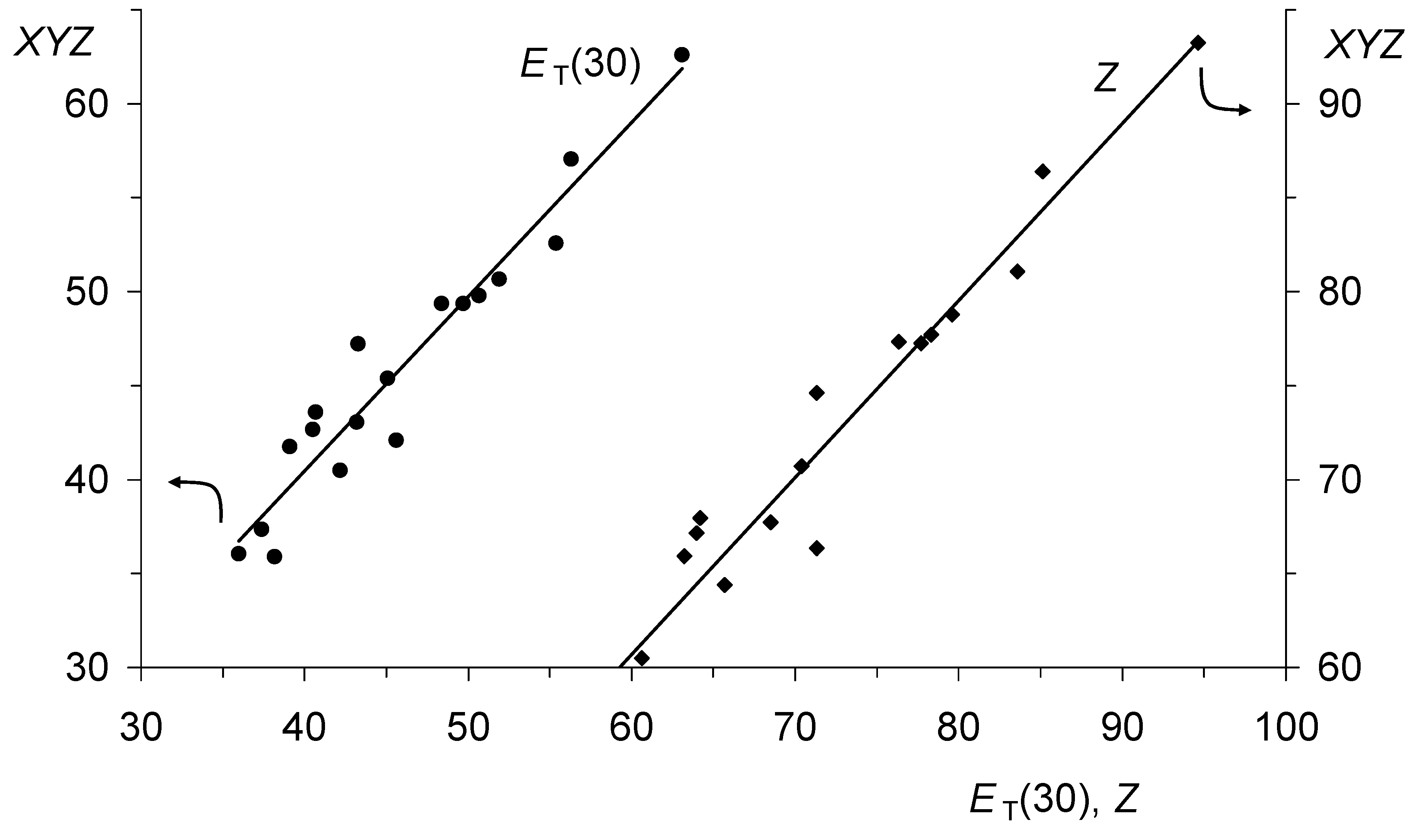
Figure 10.
Linear correlations between the ET(30) and the Z scale, respectively, as the abscissa and the adjusted XYZ scale of Kamlet and Taft as ordinate. Slope 0.927 for ET(30) has a correlation number of 0.96 (18 measurements; circles), a standard deviation of 2.0, and a coefficient of determination of 0.93, where the parameters are s = 16.9, a = 15.6, b = 4.5, and XYZ0 = 25.1. Slope 0.943 for Z has a correlation number of 0.97 (18 measurements; diamonds), a standard deviation of 2.4, and a measure of determination of 0.94, where the parameters are s = 20.8, a = 21.2, b = 7.0, and XYZ0 = 44.6.
Figure 11.
Linear correlations between the ET(30) and the Z scale, respectively, as the abscissa and the fitted Catalán’s A scale as the ordinate. Slope 0.985 for ET(30) with a correlation number of 0.98 (18 measurements, circles), a standard deviation of 1.6 and a coefficient of determination of 0.96, with parameters are b = 21.4, c = 4.27, d = 5.05, e = 12.7, and A0 = 25.1. Slope 0.984 for Z with a correlation number of 0.98 (18 measurements. diamonds), a standard deviation of 2.1 and a measure of determination of 0.96 where the parameters are b = 28.6, c = 7.40, d = 5.08, e = 16.6, and A0 = 44.6.
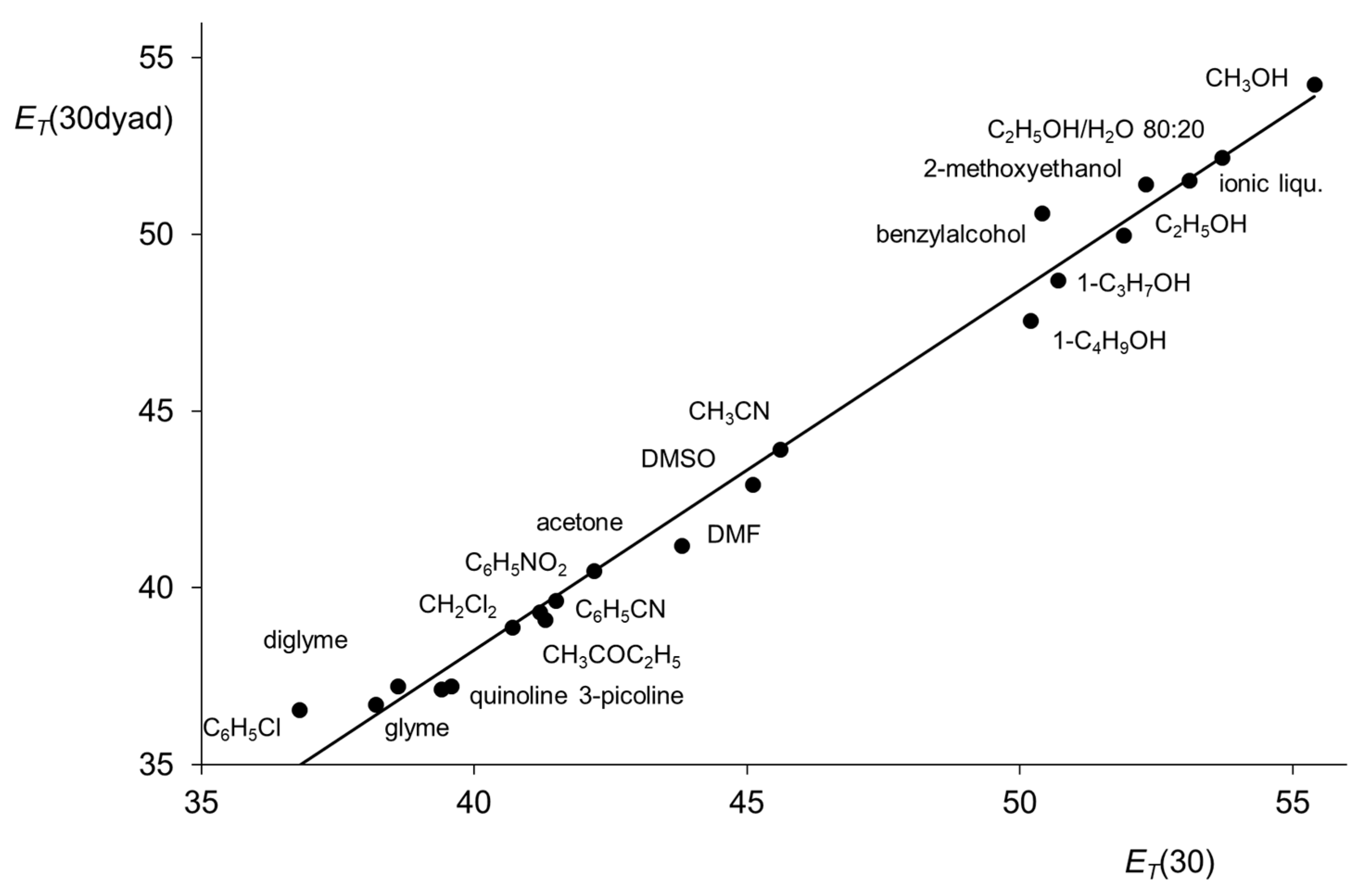
Figure 12.
Linear correlation between the
ET(30) values of betaine
3 and
ET(30dyad) values of dyad
11 for various solvents [
58] (ionic liqu.: 1-butyl-3-methylimidazolium-tetrafluoroborate). Slope 1.02, intercept −2.43, correlation number 0.993 for 20 points, standard deviation 0.7, coefficient of determination 0.987.
Figure 13.
Linear correlation between
ET(30) values of betaine
3 and the
ET(30diam) values of dyad
13 for various solvents [
58]. Slope 1.008, intercept −1.33, correlation number 0.9989 for 12 points, standard deviation 0.3, coefficient of determination 0.998.
Figure 13.
Linear correlation between
ET(30) values of betaine
3 and the
ET(30diam) values of dyad
13 for various solvents [
58]. Slope 1.008, intercept −1.33, correlation number 0.9989 for 12 points, standard deviation 0.3, coefficient of determination 0.998.
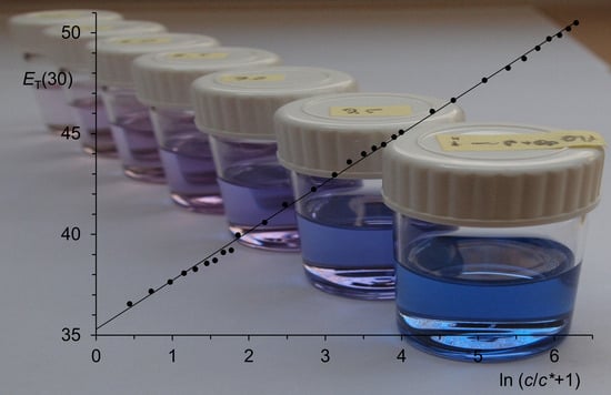
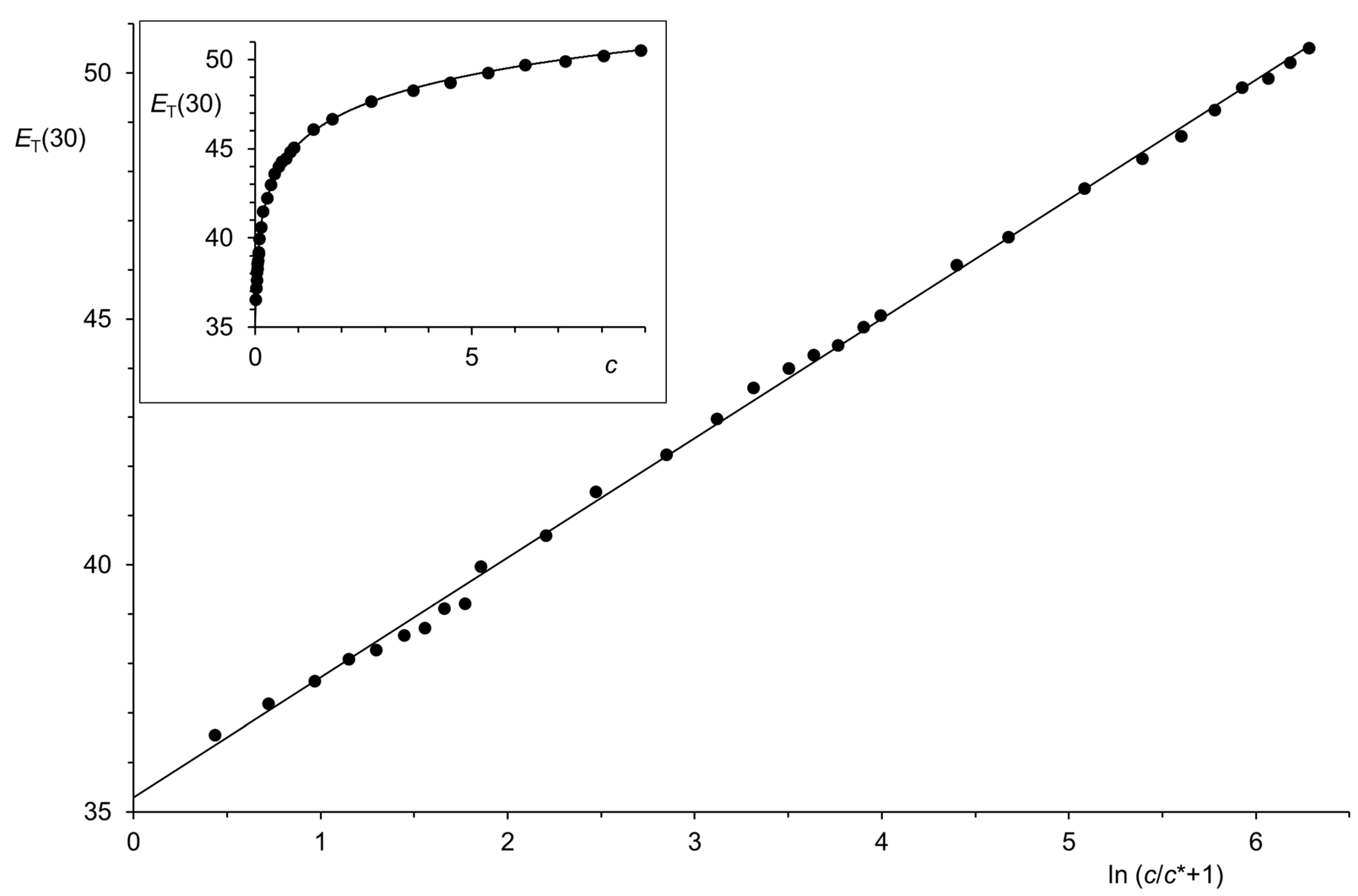
Figure 14.
Linear correlation between the
ET(30) values of the mixture
N-
tert-butylformamide/benzene [
87] and ln (
c/
c* +1) where
c is the molar concentration of the former and
c* = 0.0167 mol·L
−1; slope
E = 2.43 kcal·mol
−1, intercept
ET(30)
0 = 35.3 kcal·mol
−1, correlation number
r = 0.9993, coefficient of determination
r2 = 0.999, standard deviation
σ = 0.17 kcal·mol
−1. Inset:
ET(30) values of the mixture
N-
tert-butylformamide/benzene as a function of the concentration
c in mol·L
−1 of the former: Measured
ET(30) values (filled circles) and the calculated with Equation (14) (solid curve).
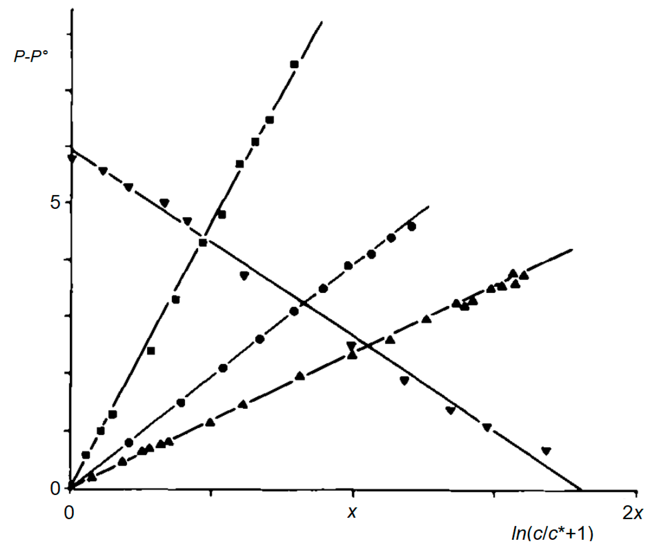
Figure 15.
Linear relationship between P and ln (c/c* + 1) for various polarity scales according to Equation (5). Diamonds: P = ET(30) (methanol/acetone); x = 2. Circles: P = Y (water/methanol); x = 1. Squares: P = Z (methanol/acetone); x = 2. Triangles: P = π1* (ethanol/n-heptane); x = 1, ordinate: P − P° + 5.9.
Figure 16.
Linear correlation between
ln (
c/
c* + 1) and the
ET(30) values of the mixture water/1.4-dioxane [
87] (
c* = 0.48 mol·L
−1; measured values as filled circles; linear correlations as lines) as a function of the concentration
c of water. Left correlation:
E = 4.27, intercept 35.6, standard deviation 0.2, correlation number
r = 0.9992 for 27 measurements, measure of determination
r2 = 0.998, extrapolation with the dashed line. Right correlation:
E = 11.1, intercept 8.26, standard deviation 0.2, correlation number
r = 0.997 for 8 measurements, measure of determination
r2 = 0.993. Inset top left:
ET(30) values of the water/1,4-dioxane mixture as a function of the water concentration
c, curves for calculated
ET(30) values, dashed curve for extrapolation. Inset bottom right:
ET(30) values of water/1,4-dioxane as a function of
ln c; The two linear correlations are already obvious in a simple logarithmic plot because of the low values of
c*.
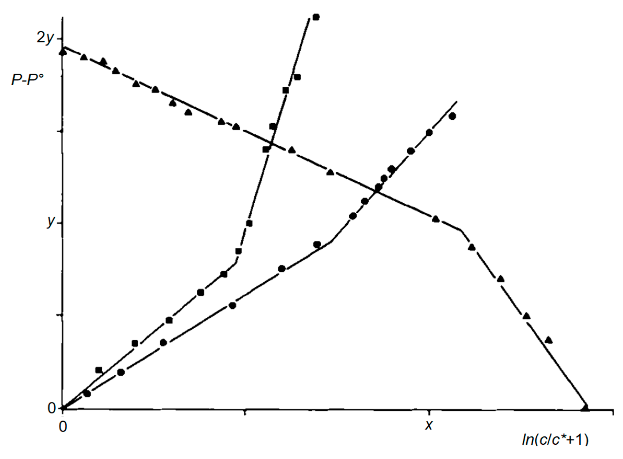
Figure 17.
Double linear correlations according to Equation (5) for the water/ethanol mixture and different polarity scales. Filled circles: P = Y (x = 2, y = 1); filled squares: P = ET(1) (x = 1, y = 4); filled triangles: P = π1* − 7.7 (x = 1, y = 4).
Figure 17.
Double linear correlations according to Equation (5) for the water/ethanol mixture and different polarity scales. Filled circles: P = Y (x = 2, y = 1); filled squares: P = ET(1) (x = 1, y = 4); filled triangles: P = π1* − 7.7 (x = 1, y = 4).
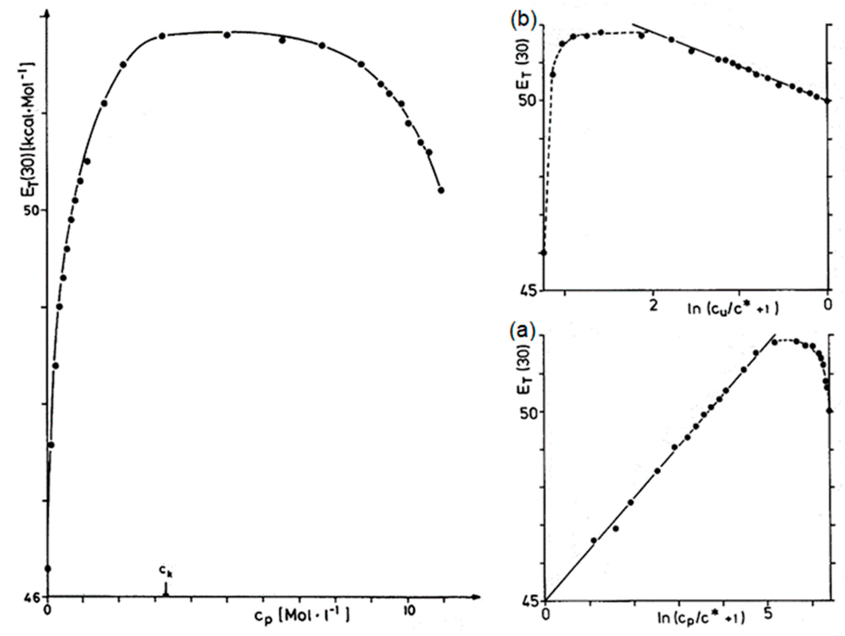
Figure 18.
ET(30) values of mixtures of 1-butanol/nitromethane [
91]. (
Left)
ET(30) values of the mixture nitromethane/1-butanol as a function of the molar concentration
cp of 1-butanol; the maximum is exceeded at
ck = 3.3 mol·L
−1. (
Bottom right (
a)): Linear correlation between
ET(30) and ln (
cp/
c* + 1) with
cp as the molar concentration of 1-butanol as the solid line and deviations to lower values after passing
ck shown as dashed curve; (
Top right (
b)): Linear correlation between
ET(30) and ln (
cu/
c* + 1) with
cu as the molar concentration of nitromethane as solid line and deviations to lower values after passing
ck shown as dashed curve.
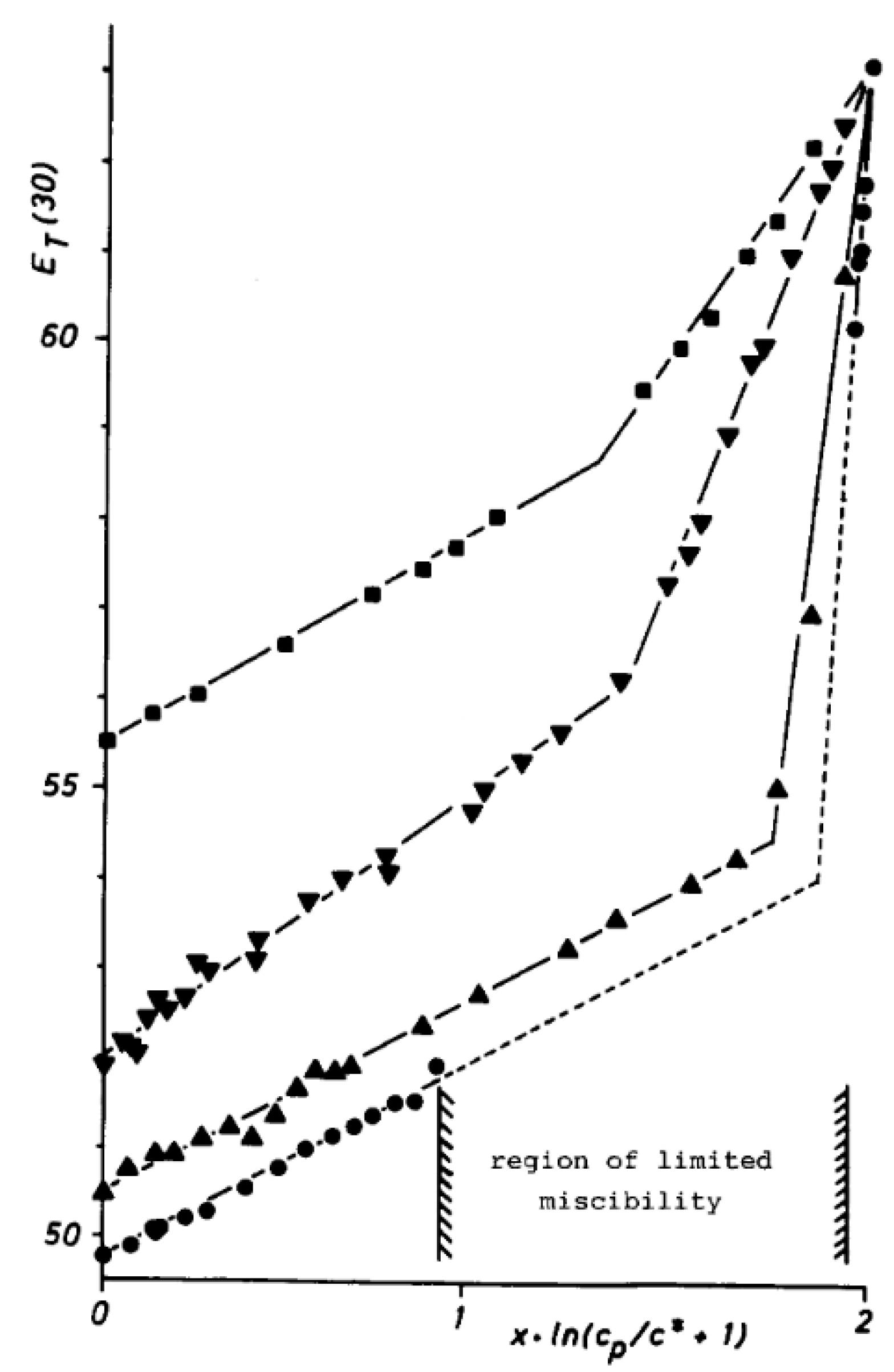
Figure 19.
ET(30) values of binary mixtures between
n-alkanols and water as a function of ln (
cp/
c* + 1) according to Equation (5) with
cp as the concentration of the polar water [
94]; the ordinate was scaled by
x to obtain a uniform value for water. Squares: water/methanol (
x = 0.157); some values are taken from ref. [
47]. Triangles down: water/ethanol (
x = 0.318); some values are taken from ref. [
47]. Triangles up: water/1-propanol (
x = 1.349). Circles: water/l-butanol (
x = 1.705). Solid lines result from application of Equation (5) and least squares method; dashed lines are extrapolations into the region of limited miscibility.
Figure 20.
(
Left)
ET(30) values [
56] of homologous linear 1-alkanols as a function of the logarithm of their molar concentration
cp. Their chain lengths
n are given in parenthesis such as (0) for water and (1) for methanol. (
Right) Comparison of
ET(30) values as a function of the logarithm of the molar concentration of OH groups (range of low concentrations of OH groups). Circles: Pure linear 1-alkanols, triangles: Mixtures of ethanol and 1,4-dioxane, squares: Mixtures of ethanol and
n-heptane.
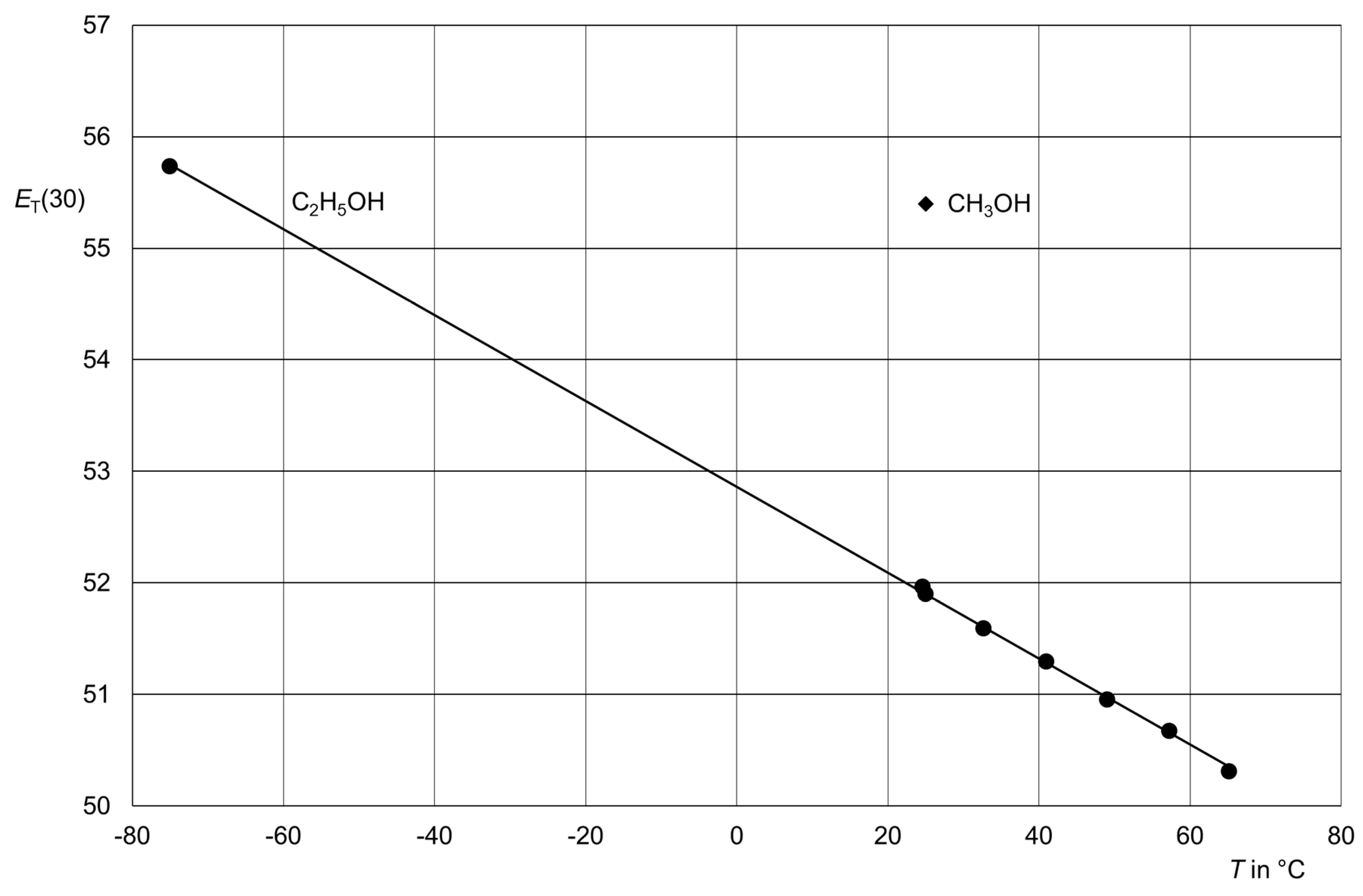
Figure 21.
Thermochromism of
3 in ethanol: Filled circles for the measurements (measurements were taken from ref. [
99]) and a filled diamond for the polarity of methanol at room temperature for comparison. Linear correlation between
T and
ET(30): slope −0.0385, intercept 52.859, correlation number −0.99988 (7 measurements), coefficient of determination 0.9998, standard deviation 0.03.
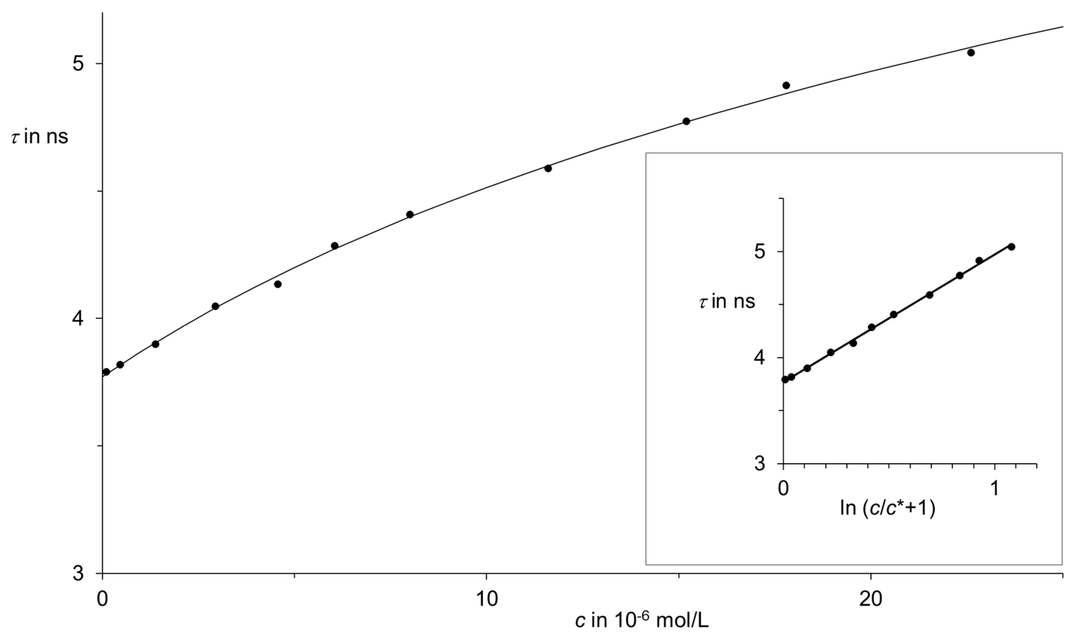
Figure 22.
Dependence of the fluorescence lifetime τ on concentration c of highly diluted solutions of the fluorescence dye S-13 (RN 110590-84-6) in chloroform: Measurements as filled circles; curve calculated by means of Equation (5). Inset: linear correlation between τ and (ln c/c* + 1) according to Equation (5): E = 1.199; c* = 1.17·10−5 mol/L; correlation number 0.9992 (11 measurements); coefficient of determination 0.998; standard deviation 0.02.
Figure 23.
(Left) Linear correlation between the density ρ and ln (cp/c* + 1) according to Equation (5); every second measurement is recorded in the graphics for clarity (all measurements were used for calculations); slope 0.174, intercept 0.79093; c* = 24.5, correlation number 0.999947 for 71 measurements; coefficient of determination 0.9999. (Right) Linear correlation between the index of refraction over the density nD20/ρ and ln (cp/c* + 1) according to Equation (5); every second measurement is plotted for clarity; slope −0.257, intercept 1.6797; c* = 19.9, correlation number −0.99998 for 71 measurements; coefficient of determination 0.99996.


