Prediction of the Structural Color of Liquid Crystals via Machine Learning

Abstract

Materials that generate structural color may be promising alternatives to dyes and pigments due to their relative long-term stability and environmentally benign properties. Liquid crystal (LC) mixtures of cholesteryl esters demonstrate structural color due to light reflected from the helical structure of the self-assembled molecules. The apparent color depends on the pitch length of the liquid crystal. While a wide range of colors have been achieved with such LC formulations, the nature of the pitch–concentration relationship has been difficult to define. In this work, various machine learning approaches to predict the reflected wavelength, i.e., the position of the selective reflection band, based on LC composition are compared to a Scheffe cubic model. The neural network regression model had a higher root mean squared error (RMSE) than the Scheffe cubic model with improved predictions for formulations not included in the dataset. Decision tree regression provided the best overall performance with the lowest RMSE and predicted position of the selective reflection band within 0.8% of the measured values for LC formulations not included in the dataset. The predicted values using the decision tree were over two-fold more accurate than the Scheffe cubic model. These results demonstrate the utility of machine learning models for predicting physical properties of LC formulations.

1. Introduction

Structurally colored materials may be promising alternatives to dyes and pigments because they have relatively long-term stability and environmentally benign properties [1,2]. Liquid crystals are one class of materials that can demonstrate structural color [3,4]. For liquid crystals, the color is attributed to selective reflection from the liquid crystalline structure. Specifically, the liquid crystal molecules self-assemble into a periodic helical structure with a repeat distance (pitch length) of the order of the wavelength of light [5]. Practically, coatings (>10–20 microns) demonstrate iridescent colors similar to those observed in some beetles and butterflies [6]. Using formulations of cholesteryl esters, a wide range of colors have been achieved [6]. An important measure of the bright color observed is the position of the selective reflective band (experimentally measured at normal incidence) [5]. Methods to tune the position of the selective reflection band are of interest for a broad range of applications including filters, lenses, reflectors, and light shutters [7,8]. Traditionally, liquid crystal devices consist of a thin layer of liquid crystal material between glass substrates [8]. There has been growing interest in processing freestanding liquid crystal materials for graphics applications [8]. Applications in security labels and anti-counterfeiting technologies as well as lens fabrication have also been reported [7]. Liquid crystal films have been used as sensors for lipids and other biomolecules [9] as well as flow sensors [10]. LC coatings on aluminum plates have also been used for flow visualization and for measuring shear stresses over planar surfaces in flow, e.g., flows around cylinders [11]. Application of liquid crystals in painting or sculpture [12] as well as coatings of fibers [13] has also been proposed.

Predictive relationships between the position of the selective reflection band and composition may be a useful tool in reducing experimental ad hoc approaches that are time-consuming and expensive; models based on linear additivity have not matched experimental data [14,15]. Multivariate data analyses of formulation and process development have been of growing interest [16,17]. Generally, the two approaches to improve understanding of formulation have been experimental design methodology (response surface) as well as data mining with machine learning. Machine learning can be used when experimental design models do not have sufficient density in the parameter space to capture the nonlinearities of the system [17,18,19]. Machine learning techniques, e.g., artificial neural networks, can be used to predict the product properties from a set of ingredients and/or process conditions. Such approaches can be considered complementary to experimental design [17].

Machine learning has been a useful tool in characterization and application of liquid crystals. For characterization, classification of liquid crystal phase based on polarized optical microscopy videos/images has also been performed using supervised machine learning. Using neural networks, the complexity of the architecture needed for classification depended on the complexity of the phase transition (e.g., Iso-SmA-Cryst (simple) vs. Iso-N-SmA-SmB-SmE-Cryst (more complex)) [20,21]. Characterization of liquid crystals via texture observation using machine learning has also enabled automated classification of ferroelectric phases [22]. Machine learning has also been leveraged to facilitate the use of liquid crystals in sensing applications. For example, machine learning has been used to automate processing of polarized light microscopy images of liquid crystals for the detection of Cd²⁺ ions. Based on the brightness of the image, neural networks were used to distinguish positive and negative areas that are triggered by anchoring transitions of the liquid crystals [23]. Ordering transitions induced by dimethyl-methylphosphonate (DMMP) in the gas phase using liquid-crystal-filled microwells have also been analyzed using machine learning. RGB images were processed using a convolutional neural network to classify the presence of DMMP (positive) or water (negative). Ten features were used to automatically identify differences in the texture in the presence of DMMP [24,25]. In other applications, images of shear-sensitive coatings have been analyzed with machine learning to determine the magnitude and direction of the shear stress based on the observed color [11]. Machine learning has also been used for detection of oil droplets in inhomogeneous smectic liquid crystal films based on images [26]. Scattering patterns of liquid crystal droplets in flow cytometry have also been analyzed using a machine learning approach to identify lipopolysaccharides from three bacterial organisms and predict their concentration in aqueous media. Concentrations as low as 10 fg/mL were detected based on subtle differences in the scatter fields [27].

Machine learning has been used to predict the dielectric properties of nematic liquid crystal composite structures (dye-doped) based on input processing parameters (frequency, voltage, and dispersion rate) and measurements of the dielectric constant [28]. Machine learning has been used to characterize liquid crystal properties based on the material structure. For example, elastic constants have been determined from polarized light microscopy images of nematic liquid crystals [29]. Transmittance and luminance have also been predicted based on polarized optical microscopy images. The crosslinker concentration, irradiation temperature, and irradiation intensity were found to be important fabrication parameters affecting the thermoresponsive changes in transmittance [30]. The pitch of cholesteric textures of nematic liquid crystals of 5CB has been predicted based on a combination of simulations and machine learning [31,32]. These studies demonstrate the utility of machine learning for predicting properties of liquid crystals based on fabrication and processing parameters. However, predicting the effect of component concentration on the position of the selective reflection band using machine learning has yet to be demonstrated.

In this work, experiments were performed to build a dataset of the position of the selective reflection band for various compositions of ternary blends of cholesteryl ester coatings. Various machine learning approaches (neural networks and decision tree analyses) were used to predict the position of the selective reflection band (wavelength in nm) based on the component concentrations (weight fractions of each component). The results were compared to experimental mixture design using a Scheffe cubic model. All models were used to predict the position of the selective reflection band of formulations not included in the dataset to compare the predictive capabilities of the models.

2. Materials and Methods

2.1. Liquid Crystal Formulation

Liquid crystal components: cholesteryl oleyl carbonate (COC), cholesteryl pelargonate (CP), and cholesteryl chloride (CC) were obtained from Sigma (St. Louis, MO, USA). All chemicals were used as received. The components were combined in appropriate mass ratios (ternary mixtures), heated to 90 °C for ~15 min, until macroscopically homogenous, and cooled to room temperature. Samples were stored at ambient temperature.

2.2. Liquid Crystal Characterization

To characterize the reflectance spectra, each liquid crystal formulation was coated on untreated glass (borosilicate, 0.13 to 0.16 mm thick, obtained from Corning, Corning, NY, USA) via doctor blade application. Briefly, two opposite edges of the glass were secured with a single layer of tape (50–60 µm thick). A small amount of liquid crystal was placed along the top edge perpendicular to the tape. A metal blade was drawn in a single direction until the liquid crystal coating was even with the edges of the tape. Samples were analyzed with UV reflectance spectroscopy using an Ocean Optics spectrometer (Ocean Optics FLAME-S-UV-VIS with an HL-2000-FHSA light source and 400 μm reflection probe). The light source detector was placed at a 90° position. A PTFE reflectance standard was used as a reference. For each formulation, doctor-bladed samples were prepared in triplicate. The UV reflectance spectrum of each doctor-bladed sample was measured. From each UV reflectance spectrum, the wavelength at which the maximum reflectance occurred was identified as the position of the selective reflection band. Additionally, photographs of the samples were obtained. Samples were mounted on black paper and placed in a 12 inch × 12 inch × 12 inch photo light box at ambient temperature (21–23 °C). Images were captured with a smart phone using a 90° viewing angle. Samples were typically analyzed within 1 day of preparation. Samples were stored in ambient light and at ambient temperature; no visible change was observed at ambient conditions. This observation is consistent with the expectation that mixtures of COC, CC, and CP are shear-sensitive formulations, and show minimal change in appearance between 20 °C and 37 °C [33].

2.3. Mixture Design Method

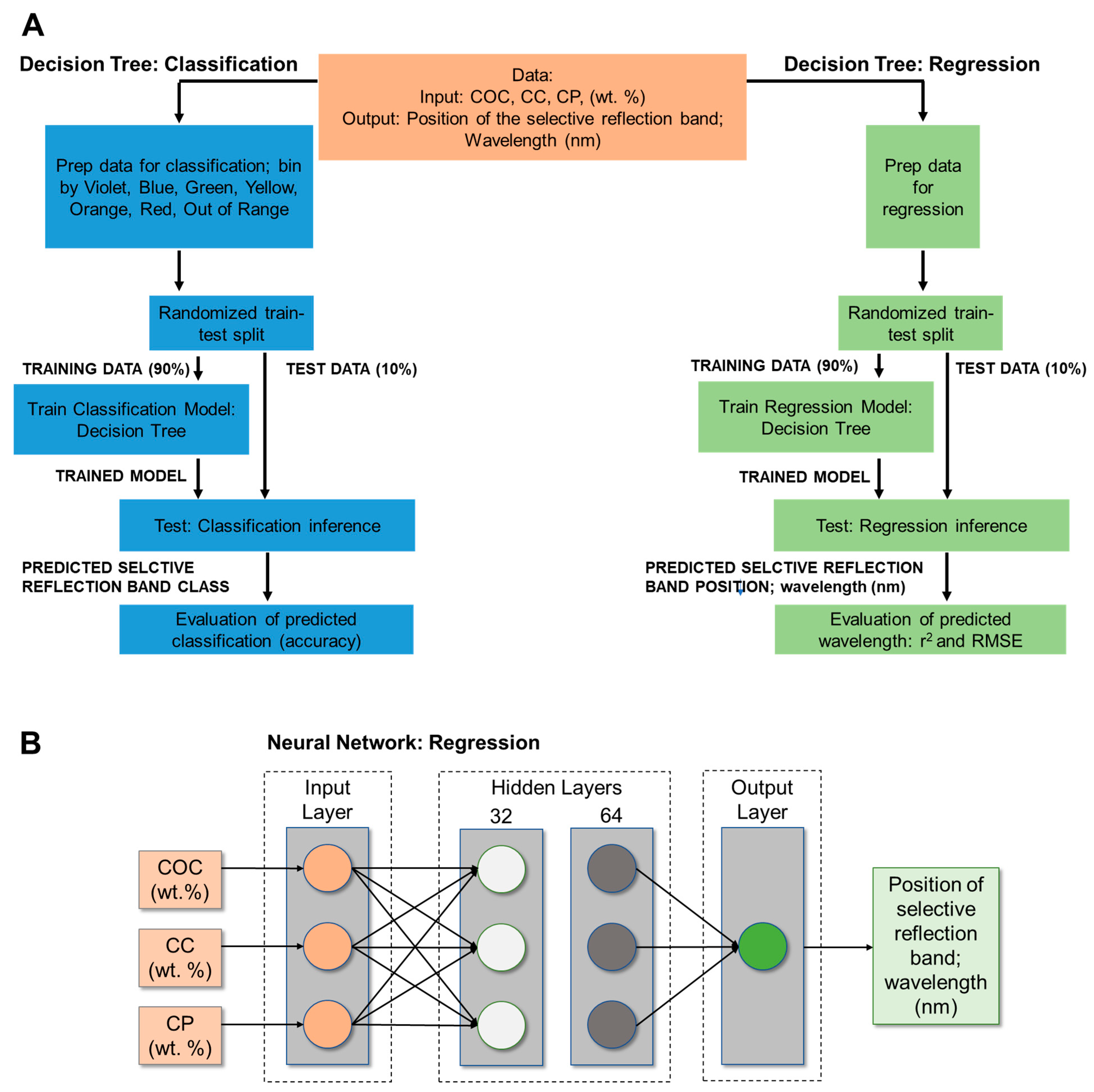
Mixtures with selective reflection bands in the visible range were included in the statistical design, i.e., a total of 33 LC formulations. The reflectance spectra were measured in triplicate for a total of 99 measured samples. The Scheffe cubic model was applied to the experimental results to determine the effect of the LC component concentration on the position of the selective reflection band. The Scheffe cubic model is of the following form:

$$E\left(Y\right)={\displaystyle \sum }_{i=1}^q{\beta }_i{x}_i+{\displaystyle \sum }_{i=1}^{q-1}{\displaystyle \sum }_{j=i+1}^1{\beta }_{i,j}{x}_i{x}_j+{\displaystyle \sum }_{i=1}^{q-1}{\displaystyle \sum }_{j=i+1}^1{\gamma }_{i,j}{x}_i{x}_j\left(x_i-x_j\right)+{\displaystyle \sum }_{i=1}^{q-2}{\displaystyle \sum }_{j=i+1}^{q-1}{\displaystyle \sum }_{k=j+1}^q{\beta }_{ijk}{x}_i{x}_j{x}_k$$

where E(Y) is the response (dependent variable to be predicted), q is the number of components, and x₁, x₂,…x_q are the component proportions subject to the mixture constraint

$${\displaystyle \sum }_{i=1}^q{x}_i=1$$

(i.e., sum of the component fractions is one), and β and γ are the fitting parameters determined from experimental data [34,35].

The analysis was performed with a confidence level of 95% with JMP Pro 16 software. The model coefficients were considered to be statistically significant for p-values < 0.05. The models for predicting position of the selective reflection band based on LC composition were obtained by eliminating nonsignificant terms.

2.4. Data Mining

As a complementary approach to the mixture design analysis using the Scheffe cubic model, data mining approaches based on multivariate data analyses were also applied. Multivariate techniques such as artificial neural networks can be used to predict product properties’ results from a given set of ingredients and process conditions. Knowledge discovery methods such as decision trees based on rough set theory can also be used to guide design of new products [17]. Thus, artificial neural networks and decision tree regression analyses were compared to the Scheffe cubic model to predict the position of the selective reflection band based on the composition of the LC formulation.

The LC formulation dataset for regression contained 33 COC:CC:CP compositions. For each formulation, the 3 measurements of reflectance were taken, and an average value of the position of the selective reflection band (wavelength in nm) was identified. Thus, the data matrix contained 3 input variables (COC wt%, CC wt%, and CP wt%, independent variables) and 1 output variable (the quality attribute, i.e., dependent variable, which in this case was the position of the selective reflection band, wavelength (nm)). Initially, the data (33 inputs with 4 features) were transferred to an Excel file. The dataset was randomly divided into training and testing subsets. The training subset contained 90% of all cases, and the testing subset contained the remaining 10% of the cases to test the predictive capability of the models. Regression models (decision tree or neural network analysis) were used to predict the position of the selective reflection band based on LC composition. To tune the reflection band within the visible range based on formulation, classification into visible color ranges based on ISO 21348 definitions [36] (violet: 360 ≤ λ_max < 450 nm, blue: 450 ≤ λ_max < 500 nm, green: 500 ≤ λ_max < 570 nm, yellow: 570 ≤ λ_max < 591 nm, orange: 591 ≤ λ_max < 610 nm, and red: 610 ≤ λ_max < 760 nm) was performed. An additional 13 measurements for formulations that did not have a peak in the visible range (out of range) were included for classification. Thus, the seven categories were violet, blue, green, yellow, orange, red, and out of range. Classification models using a decision tree classification analysis were used to visualize the formulation space to tune the position of the selective reflection band in the visible range. An overview of these methods is provided in Figure 1. These machine learning models were developed using Python version 3.10.6.

Neural network regression results were compared to the mixture design performed using the Scheffe cubic model. Artificial neural networks (ANNs) are made of connected nodes, which are each assigned a weight. The network consists of an input layer, an output layer, and hidden layer(s). The nodes in each layer use the outputs of all nodes in the previous layer as inputs, resulting in the interconnection of the layers. The assigned weights are adjusted based on the training data. This approach is considered amongst the strongest algorithms for regression tasks [37].

For neural network regression, the neural network library Keras version 2.13. was used. The networks contained 1 hidden layer with 64 units and a ‘relu’ activation function, a second feed forward layer with 32 units and a ‘relu’ activation function, and a final output layer with a single unit (no activation function). The learning rate was 0.001 and 1000 epochs (training cycles) were used. The network parameters were optimized using the Adaptive Moment Estimation (ADAM) optimization algorithm. We trained the network with 90% of the data (randomly selected) using the negative R² loss function. The model was then tested by comparing the predicted position of the selective reflection band of the remaining 10% of the data to the measured values. The performance of the regression model was quantified using the squared correlation (R²) and the root mean squared error (RMSE). The model performance was benchmarked against the results from the Scheffe cubic model. The models were further evaluated with new formulations not included in the original dataset. The predicted positions of the selective reflection bands using the regression models were determined by running each model 5 times. The average and standard deviation of the runs were reported.

In decision tree analyses, the Classification and Regression Trees (CART) algorithm creates a binary tree from the data so each internal node has exactly two branches. The inputs (independent variables) are used as the splitting criteria to form the shape and sequence of the branches to produce subsets of data that are as homogenous as possible with respect to the target variable (dependent variable). No assumptions are required about the statistical distribution of data. This approach has been used to separate important inputs from unimportant branches so that only the strongest relationships between the inputs and the target variable are retained [17]. For the decision tree analysis, scikit learn version 1.3.0 was used. The CART algorithm was used to produce a tree model. For regression, the criterion used for measuring the quality of splits was the mean squared error. The maximum depth of the tree was not explicitly limited. The minimum number of samples required to split an internal node was set to 2, and the minimum number of samples required to be in a leaf node was set to 1. Additionally, a random seed was set to 42 to ensure the random number generator produces the same sequence of random numbers for reproducibility. The default maximum number of leaf nodes as well as the minimum impurity decrease were set to None and 0.0, respectively.

For classification, the same CART algorithm and parameters were used. The criterion used for measuring the quality of splits was the ‘gini’ impurity criterion. The class weights were set to None, assuming equal. In this decision tree classification model, each terminal node’s predicted category was the visible range of the mean of the target values (selective reflection band) for records in the node based on ISO 21348 [36]. The decision trees in this analysis underwent a pruning process aimed at optimizing their complexity and avoiding overfitting. The cost_complexity_pruning_path function from scikit learn was used to prune the tree recursively based on the complexity parameter. The accuracy of the resulting classification was evaluated over 5 runs. The average and standard deviation of the accuracy were reported.

3. Results and Discussion

Ternary mixtures of COC, CC, and CP demonstrate structural color attributed to the self-assembly of the molecules into a helical structure. Coatings (>10–20 microns) demonstrate selective reflection based on the spacing between layers of molecules differing by an angle of 360° (pitch). A wide range of colors have been achieved with such LC formulations [6]. While it has been well established that when cholesteric compounds are mixed, the resultant pitch and thus the resulting reflected color depend on the concentration of the components, the nature of the pitch–concentration relationship has been difficult to define [14,15]. Linear additivity based on the weight average of each component has not been found to adequately fit experimental data [14,15,38]. The helical twisting power has also been used to relate pitch and concentration for cholesteric nematic liquid crystals, but has not been shown to apply to cholesteric–cholesteric mixtures and general multicomponent mixtures [15]. Thus, predicting pitch (and resulting apparent color) to LC composition (component concentrations) in mixtures of cholesteryl ester remains poorly understood. To better understand the effect of component concentration on resulting color and pitch length, we aimed to apply the Scheffe cubic model to the experimental results to determine the effect of LC composition on the position of the selective reflection band.

Initially, we examined the gamut of colors that were achievable with the ternary LC formulations. The COC content was varied from 90% to 30% while holding the ratio of CP:CC constant at 1:1. At 90% COC content, the LC coatings appeared transparent with a slight hint of blue/purple. Decreasing the COC content to 80% resulted in a much more vibrant sample appearing violet. Other reflected colors with longer wavelengths were observed by further decreasing the COC content. For example, a blue sample was observed at 70% COC, a green sample was observed at 60% COC, a yellow sample was observed at 50% COC, an orange sample was obtained at 44% COC, and a red sample was observed at 38% COC (based on ISO 21348 [36]). When the COC content was below 38% and above 80%, the samples became more transparent. Photographs of the samples taken at a 90° viewing angle against a black background and their reflectance spectra are shown in Figure 2.

Briefly, we demonstrated that the formulations achieved here can be used as structurally colored paints. The formulations were painted on a black polyethylene substrate and imaged under ambient lighting conditions (Figure 3). When applied with a paint brush, the apparent color matched the color predicted with the reflectance measurements. This experiment confirms that the position of the selective reflective band (experimentally measured at normal incidence) is an important measure of the bright color observed.

Formulations that were colorless and did not show a reflection peak in the visible range were also identified to further confine the parameter space. For example, a 50:50 binary mixture of COC:CC did not show visible color. Based on these initial formulations, 33 LC formulations (ternary mixtures) that reflected visible color were prepared. Coatings from each formulation were prepared in triplicate for analysis with reflectance spectroscopy. Photos were also taken from a 90° viewing angle against a black background. The average RGB of the sample was determined from the image. These formulations are shown in Figure 4 with the symbols colored using the RGB from the images of the coatings.

Experimental data for the position of the selective reflection band were fitted using the Scheffe cubic model to obtain a relationship between the position of the selective reflection band and the formulation composition (weight fractions of each component). Using the Scheffe cubic model, an R² greater than 0.99 was obtained, which indicates a strong correlation between the predicted and actual values. Overall, the root-mean-square error (RMSE) was 4.42 nm (n = 99). Further, the model has a p-value of <0.0001, indicating its statistical significance.

The regression coefficients as well as the variance analysis of the effect of each LC formulation component (X_COC, cholesteryl oleyl carbonate; X_CC, cholesteryl chloride; X_CP, cholesteryl pelargonate) are shown in

Table 1. Regression coefficients of the Scheffe cubic model to predict the position of the selective reflection band based on the liquid crystal composition.

Effect	Coefficient Estimate ± Standard Error	p-Value
XCOC	394 ± 3	<0.0001
XCC	6984 ± 434	<0.0001
XCP	451 ± 66	<0.0001
XCOCXCC	−8067 ± 749	<0.0001
XCOCXCP	102 ± 108	0.35
XCCXCP	−9954 ± 766	<0.0001
XCOCXCC(XCOC − XCC)	1998 ± 355	<0.0001
XCOCXCP(XCOC − XCP)	−141 ± 61	0.0226
XCCXCP(XCC − XCP)	−3728 ± 714	<0.0001
XCOCXCCXCP	3100 ± 880	0.0007

. Based on the p-values, all coefficients were statistically significant (p < 0.05) except the X_COCX_CP quadratic term. The significant nonlinear terms indicate that the use of the cubic Scheffe model was necessary [35]. Examining the coefficients, the cubic X_COCX_CCX_CP blending term was synergistic (>0). In contrast, the quadratic mixing terms, i.e., X_COCX_CC and X_CCX_CP were antagonist (<0). Interestingly, while the CC-CP cubic blending term was antagonistic, the cubic COC-CC blending term was synergistic. A combination of synergistic and antagonistic blending terms has been observed when predicting the effect of composition on yield of biocrude [39] as well as predicting the octane number of fuel mixtures [40]. For this system, the combination of antagonist and synergistic blending terms may indicate the intermolecular interactions affecting molecular self-assembly of the cholesteric mesophase [38]. Notably, the value of the COC-CP (cubic) blending term was relatively small compared to the other nonlinear terms, suggesting COC-CP interactions had a relatively small effect on the position of the selective reflection band.

The limits of the model equation, i.e., single component systems, were also of interest, as an indication of the “intrinsic pitch” of the components. For example, for X_CP = 1 and assuming an index of refraction of 1.5 [41], the pitch length of the liquid crystal would be ~300 nm. This pitch length was slightly larger than reported values for the experimentally measured pitch length of CP (pitch length of 240 nm) [42]. In contrast, the model predicted a much higher dependence on CC concentration. In the limit of X_CC = 1 and assuming an index of refraction of 1.4 [40], the pitch length of the liquid crystal would be 4700 nm. This pitch length was an order of magnitude higher than the experimentally measured pitch length of CC (pitch length of 340 nm) [42]. Differences in the “intrinsic pitch” indicated by models and the experimentally measured pitch lengths have been observed with mixtures of cholesteryl esters and indicated non-ideal behavior [38]. For cholesteryl ester mixtures, crystal packing and disparate molecular volumes of the components can result in such non-ideal behavior [43].

The utility of the Scheffe cubic model for predicting the position of the selective reflection band of formulations not included in the dataset was evaluated. New formulations were prepared: a 20:25:55 COC:CC:CP and 30:20:50 COC:CC:CP. The predicted positions of the selective reflection bands were slightly lower, 540.4 ± 0.1 nm and 482.3 ± 0.1 nm, respectively (within the same color range based on ISO 21348 [36]). Differences of 9.5 nm to 16.5 nm may be of practical importance near the boundaries of the color ranges (e.g., between green and blue or yellow and green).

Machine learning was investigated as a tool to improve prediction of the position of the selective reflection band of LC formulations. Neural network regression and a decision tree regression analysis were compared to mixture design. A neural network regression analysis was performed. The model was trained with 90% of the data (randomly selected). The performance of the model on the training data (R² and RMSE) as a function of epochs (training cycles) is shown in Figure S1. While R² > 0.99 can be achieved with 500 epochs (~500), the RMSE is relatively high (>15) and three-fold higher than the Scheffe cubic model. Increasing the epochs from 500 to 1000, the RMSE decreased by ~two-fold; suggested increased epochs of learning were beneficial. To check for potential overfitting, the R² on the training data (90%) was compared to the R² on the testing data (10%). Both values were >0.99. This approach is considered appropriate for regression with small datasets [44]. Evaluating the performance of the trained neural network regression model on the testing data, an R² greater than 0.99 was obtained, indicating a strong correlation between the predicted and actual values and the RMSE was 7.12 (

Table 2. Summary of test statistics comparing Scheffe cubic model, decision tree (test data), and neural network regression (test data).

	R2	RMSE
Scheffe Cubic Model	0.99898	4.42
Decision Tree	0.99904	2.79
Neural Networks	0.99694	7.12

). The R² was comparable to the Scheffe cubic model, while the difference between the predicted values and measured values was 1.6-fold higher using the neural network regression compared to the Scheffe cubic model (as indicated by the RMSE).

Using the same dataset, a decision tree regression analysis was performed. From the analysis performed, the effect of the LC composition on the resulting position of the selective reflection band can be depicted in the form of a tree graph (Figure 5). The model obtained can provide insights into the relations in the complex dataset and can be considered complementary to the experimental design [17]. Interestingly, the CC concentration was the only variable in the first two levels (I–II) of the decision tree (which eventually were then further divided by position of the selective reflection band, e.g., red range to blue range depending on COC and CP concentration). This result is in agreement with the coefficients from the Scheffe cubic model in which the coefficient for X_CC is an order of magnitude greater than X_COC and X_CP.

It is also interesting to note that the position of the selective reflection band in the red region could be differentiated in the fewest levels (levels I–V). In contrast, the position of the selective reflection band in the violet region required the most levels (level IX). Positions in the purple, blue, and green ranges were differentiated in level V of the tree. In comparison, differentiation in the yellow, green, and orange ranges required an additional level of complexity (level VI). The position of the selective reflection bands at the lowest wavelengths in the visible spectrum was differentiated only by CC concentration (X_CC < 3.25 wt.%). Formulations with selective reflection bands in the violet range with peak reflectance wavelengths <422.7 nm were differentiated by CC concentration followed by COC concentration. For formulations with selective reflection bands in the blue range, the positions of the selective reflection bands were differentiated by CC concentration followed by CP concentration. The differentiation among the positions of the selective reflection bands in the other color regions (e.g., green, yellow, orange) was based on CC concentration, followed by CP and/or COC concentrations.

In order to evaluate the accuracy of the prediction, the positions of the selective reflection bands predicted with the model were compared to experimentally measured values using the correlation coefficient. For the training dataset, the R² was greater than 0.99 with a RMSE of 2.79, which was 1.6-fold lower than the Scheffe cubic model and 2.5-fold lower than the neural network regression. This result, i.e., that the decision tree provided the best performance, is consistent with previous results comparing machine learning methods to optimize process parameters in pellet manufacturing [17] to achieve spherical particles as well as models to predict concentration of a fluorescent dye from images [37].

To demonstrate the utility of the models, the position of the selective reflection band of two LC formulations not included in the dataset was predicted and compared to the measured values (

Table 3. Predicted positions of the selective reflection bands for formulations not in the dataset to validate the models compared to the measured values.

Formulation COC:CC:CP	Predicted Value (Scheffe Cubic Model)	Predicted Value (Neural Network)	Predicted Value (Decision Tree)	Measured Value
20:25:55	540.4 ± 0.1	549.6 ± 1.1	553.1 ± 7.1	549.9 ± 0.1
30:20:50	482.3 ± 0.1	504.8 ± 3.3	502.6 ± 1.0	498.8 ± 0.2

). The formulations not included in the dataset were 20:25:55 COC:CC:CP and 30:20:50 COC:CC:CP. The difference between the model prediction using the decision tree regression and the measured value was 0.6–0.8%. In contrast, the prediction using the Scheffe cubic model was 1.7–3.3% lower than the measured values. For example, for the 30:20:50 COC:CC:CP formulation, the difference between the Scheffe cubic model prediction and the measured value was 3.3%. For the 20:25:55 COC:CC:CP formulation, there was a 1.7% difference between the Scheffe cubic model prediction and the measured value. The accuracy of the neural network prediction depended on the formulation. For example, for the 30:20:50 COC:CC:CP formulation, the prediction accuracy using the neural network was 1.2%. The predicted value for the 20:25:55 COC:CC:CP formulation was less than 0.1%. Notably, in terms of prediction, the neural network predictions for the position of the selective reflection band appeared to be reproducible. Over the five runs, the standard deviation of five runs was within 0.6% of the predicted value. Further, the model was able to predict selective reflection band position for new formulations not included in the dataset to within 1.2% of the measured values, demonstrating the generalizability of the model to new, unseen data. These results suggested that the approaches may be complementary. In particular, neural network regression may be useful to improve the accuracy of predictions in regions where the uncertainty using the decision tree was relatively large (e.g., ~550 nm).

To visualize the formulation space to tune the position of the selective reflection band in the visible range, classification into ranges of the visible color spectrum (violet, blue, green, yellow, orange, and red) based on ISO 21348 [36] (violet: 360 ≤ λ_max < 450 nm, blue: 450 ≤ λ_max < 500 nm, green: 500 ≤ λ_max < 570 nm, yellow: 570 ≤ λ_max < 591 nm, orange: 591 ≤ λ_max < 610 nm, and red: 610 ≤ λ_max < 760 nm) was performed. An additional 13 measurements for formulations that did not have a peak in the visible range (out of range) were included. Thus, the seven categories were violet, blue, green, yellow, orange, red, and out of range.

As expected, the classification is small relative to the regression tree, approximately half the size (Figure 6). Similar to the regression tree, X_CC is in the decision for the root node (level I). Further, the CC concentration is the only variable in the first two levels of the decision tree (to further divide by position of the selective reflection band, e.g., red range and blue range depending on COC and CP concentration). CC and CP concentrations are needed to differentiate between the violet range and the blue range. CC, CP, and COC concentrations are needed to differentiate the other color ranges. Notably, yellow and orange ranges could not be differentiated using this classification model. Overall, the accuracy of classification was 90.00 ± 0.03% over five runs.

Practically, this classification is useful, achieving LC formulations with a selective reflection band within a desired range. Thus, we visualized the formulation space on ternary diagrams. For example, using the mathematical equation achieved from the Scheffe cubic model, the position of the selective reflection bands for all permutations (1% increments) was predicted, classified into violet, blue, green, yellow, orange, red, or out of range based on ISO 21348 [36], and plotted on a ternary diagram with the color of the symbol indicating the predicted color range associated with the position of the selective reflection band of the formulation (Figure 7). The operating window to achieve yellow or orange formulations appears to be relatively small due to the narrowly defined wavelength ranges (~20 nm). The formulation space visualized with the decision tree classification analysis was comparable to the Scheffe cubic model with more discrete boundaries. Additionally, more out-of-range regions were predicted at each vertex of the triangle, likely due to the additional out-of-range data that were included in the dataset for classification. Practically, the formulation space achieved from the decision tree classification analysis is able to more accurately predict the experimentally achieved selective reflection bands, especially at low CC concentrations.

We anticipate these diagrams will be a useful tool for achieving LC formulations with a tunable selective reflection band (position). Further work to relate the position of the selective reflection band to perceived structural color (e.g., hue, etc.) using various color spaces is of interest. Since additional output variables are predicted, an expanded dataset with additional unique formulations is needed. Modern machine learning techniques (e.g., few-shot learning) for cases with sparse data are also being considered. Additionally, the machine learning methods are versatile and can be expanded for other liquid crystal properties of interest. For example, the responsive optical properties are often of interest for sensors/biosensors [9,45,46], smart glass/window applications [47,48], advanced displays [49,50], and other liquid-crystal-based devices such as spatial light modulators [51,52]. Predictive relationships between functional properties such as response time or temperature-dependent properties and liquid crystal composition and processing can be developed from measurements or reports of the properties of interest [17,30].

4. Conclusions

Overall, the decision tree regression improved prediction of the position of the selective reflection band compared to the Scheffe cubic model by over two-fold. While the predictions of the position of the selective reflection band using a mixture analysis are within 0.8% using a decision tree regression analysis, the difference in predicted and measured wavelength may have practical importance near the boundaries of the color (e.g., between green and blue ranges or yellow and green ranges). This effect may be especially important for achieving formulations with selective reflection bands in the yellow and orange wavelength ranges (narrowest range of wavelengths). We note that neural network regression may be useful to improve the accuracy of predictions in regions where the uncertainty using the decision tree is relatively large (e.g., ~550 nm). To further improve the accuracy of the predictions, additional training data may be useful. Taken together, the results demonstrate that machine learning provides useful tools for predicting the properties of liquid crystal formulations.

References

1. Xuan, Z.; Li, J.; Liu, Q.; Yi, F.; Wang, S.; Lu, W. Artificial Structural Colors and Applications. Innovation 2021, 2, 100081. [Google Scholar] [CrossRef]
2. Schertel, L.; Magkiriadou, S.; Yazhgur, P.; Demirörs, A.F. Manufacturing Large-Scale Materials with Structural Color. Chimia 2022, 76, 833–840. [Google Scholar] [CrossRef]
3. Daqiqeh Rezaei, S.; Dong, Z.; You En Chan, J.; Trisno, J.; Ng, R.J.H.; Ruan, Q.; Qiu, C.W.; Mortensen, N.A.; Yang, J.K.W. Nanophotonic Structural Colors. ACS Photonics 2021, 8, 18–33. [Google Scholar] [CrossRef]
4. Sol, J.A.H.P.; Sentjens, H.; Yang, L.; Grossiord, N.; Schenning, A.P.H.J.; Debije, M.G. Anisotropic Iridescence and Polarization Patterns in a Direct Ink Written Chiral Photonic Polymer. Adv. Mater. 2021, 33, 2103309. [Google Scholar] [CrossRef] [PubMed]
5. Sage, I. Thermochromic Liquid Crystals in Devices. In Liquid Crystals, Applications and Uses; Bahadur, B., Ed.; World Scientific: Singapore, 1990; pp. 301–341. [Google Scholar]
6. Makow, D.M.; Sanders, C.L. Additive Colour Properties and Colour Gamut of Cholesteric Liquid Crystals. Nature 1978, 276, 248–250. [Google Scholar] [CrossRef]
7. Ma, L.L.; Li, C.Y.; Pan, J.T.; Ji, Y.E.; Jiang, C.; Zheng, R.; Wang, Z.Y.; Wang, Y.; Li, B.X.; Lu, Y.Q. Self-Assembled Liquid Crystal Architectures for Soft Matter Photonics. Light Sci. Appl. 2022, 11, 270. [Google Scholar] [CrossRef]
8. Kamal, W.; Orr, A.C.J.; Sykes, T.C.; Castrejón-Pita, A.A.; Elston, S.J.; Morris, S.M. On-Demand Pitch Tuning of Printed Chiral Nematic Liquid Crystal Droplets. Mater. Today Adv. 2023, 19, 100416. [Google Scholar] [CrossRef]
9. Popov, P.; Mann, E.K.; Jákli, A. Thermotropic Liquid Crystal Films for Biosensors and Beyond. J. Mater. Chem. B 2017, 5, 5061–5078. [Google Scholar] [CrossRef]
10. Green, A.A.S.; Dutch, E.; Qi, Z.; Briggs, C.; Park, C.S.; Glaser, M.A.; Maclennan, J.E.; Clark, N.A. A Gas Flow Meter with Linear Sensitivity Based on Freely-Suspended Nanofilms of Smectic Liquid Crystal. Appl. Phys. Lett. 2019, 114, 163705. [Google Scholar] [CrossRef]
11. Zhao, J.; Zhang, J.; Wang, B. A Learning-Based Approach for Solving Shear Stress Vector Distribution from Shear-Sensitive Liquid Crystal Coating Images. Chin. J. Aeronaut. 2022, 35, 55–65. [Google Scholar] [CrossRef]
12. Makow, D. Liquid Crystals in Painting and Sculpture. Leonardo 1982, 15, 257–261. [Google Scholar] [CrossRef]
13. Guan, Y.; Agra-Kooijman, D.M.; Fu, S.; Jákli, A.; West, J.L. Responsive Liquid-Crystal-Clad Fibers for Advanced Textiles and Wearable Sensors. Adv. Mater. 2019, 31, e1902168. [Google Scholar] [CrossRef]
14. Tai, H.S.; Lee, J.Y. Phase Transition Behaviors and Selective Optical Properties of a Binary Cholesteric Liquid Crystals System: Mixtures of Oleyl Cholesteryl Carbonate and Cholesteryl Nonanoate. J. Appl. Phys. 1990, 67, 1001–1006. [Google Scholar] [CrossRef]
15. Bak, C.S.; Labes, M.M. Pitch-Concentration Relationships in Multicomponent Liquid Crystal Mixtures. J. Chem. Phys. 1974, 62, 3066–3069. [Google Scholar] [CrossRef]
16. Bannigan, P.; Aldeghi, M.; Bao, Z.; Häse, F.; Aspuru-Guzik, A.; Allen, C. Machine Learning Directed Drug Formulation Development. Adv. Drug Deliv. Rev. 2021, 175, 113806. [Google Scholar] [CrossRef] [PubMed]
17. Ronowicz, J.; Thommes, M.; Kleinebudde, P.; Krysiński, J. A Data Mining Approach to Optimize Pellets Manufacturing Process Based on a Decision Tree Algorithm. Eur. J. Pharm. Sci. 2015, 73, 44–48. [Google Scholar] [CrossRef]
18. Yang, Y.; Ye, Z.; Su, Y.; Zhao, Q.; Li, X.; Ouyang, D. Deep Learning for in Vitro Prediction of Pharmaceutical Formulations. Acta Pharm. Sin. B 2019, 9, 177–185. [Google Scholar] [CrossRef]
19. Sun, Y.; Li, G.; Zhang, N.; Chang, Q.; Xu, J.; Zhang, J. Development of Ensemble Learning Models to Evaluate the Strength of Coal-Grout Materials. Int. J. Min. Sci. Technol. 2021, 31, 153–162. [Google Scholar] [CrossRef]
20. Dierking, I.; Dominguez, J.; Harbon, J.; Heaton, J. Testing Different Supervised Machine Learning Architectures for the Classification of Liquid Crystals. Liq. Cryst. 2023, in press. [Google Scholar] [CrossRef]
21. Dierking, I.; Dominguez, J.; Harbon, J.; Heaton, J. Deep Learning Techniques for the Localization and Classification of Liquid Crystal Phase Transitions. Front. Soft Matter 2023, 3, 1114551. [Google Scholar] [CrossRef]
22. Betts, R.; Dierking, I. Machine Learning Classification of Polar Sub-Phases in Liquid Crystal MHPOBC. Soft Matter 2023, 19, 7502–7512. [Google Scholar] [CrossRef] [PubMed]
23. Zhang, Y.; Xu, S.; Zhang, R.; Deng, Z.; Liu, Y.; Tian, J.; Yu, L.; Hu, Q.; Ye, Q. Automated Calculation of Liquid Crystal Sensing Images Based on Deep Learning. Anal. Chem. 2022, 94, 12781–12787. [Google Scholar] [CrossRef] [PubMed]
24. Cao, Y.; Yu, H.; Abbott, N.L.; Zavala, V.M. Machine Learning Algorithms for Liquid Crystal-Based Sensors. ACS Sens. 2018, 3, 2237–2245. [Google Scholar] [CrossRef] [PubMed]
25. Smith, A.D.; Abbott, N.; Zavala, V.M. Convolutional Network Analysis of Optical Micrographs for Liquid Crystal Sensors. J. Phys. Chem. C 2020, 124, 15152–15161. [Google Scholar] [CrossRef]
26. Hedlund, E.; Hedlund, K.; Green, A.; Chowdhury, R.; Park, C.S.; Maclennan, J.E.; Clark, N.A. Detection of Islands and Droplets on Smectic Films Using Machine Learning. Phys. Fluids 2022, 34, 103608. [Google Scholar] [CrossRef]
27. Jiang, S.; Noh, J.; Park, C.; Smith, A.D.; Abbott, N.L.; Zavala, V.M. Using Machine Learning and Liquid Crystal Droplets to Identify and Quantify Endotoxins from Different Bacterial Species. Analyst 2021, 146, 1224–1233. [Google Scholar] [CrossRef]
28. Yildirim Taser, P.; Onsal, G.; Ugurlu, O. Comparison of Experimental Measurements and Machine Learning Predictions of Dielectric Constant of Liquid Crystals. Bull. Mater. Sci. 2023, 46, 1. [Google Scholar] [CrossRef]
29. Zaplotnik, J.; Pišljar, J.; Škarabot, M.; Ravnik, M. Neural Networks Determination of Material Elastic Constants and Structures in Nematic Complex Fluids. Sci. Rep. 2023, 13, 6028. [Google Scholar] [CrossRef]
30. Kakiuchida, H.; Suzuki, K.; Kojima, T. Using Pretrained Machine Learning Models to Predict Luminous and Solar Transmittance Controllability of Liquid Crystal/Polymer Composites from Microstructural Images. Opt. Express 2023, 31, 29954. [Google Scholar] [CrossRef]
31. Sigaki, H.Y.D.; De Souza, R.F.; De Souza, R.T.; Zola, R.S.; Ribeiro, H.V. Estimating Physical Properties from Liquid Crystal Textures via Machine Learning and Complexity-Entropy Methods. Phys. Rev. E 2019, 99, 013311. [Google Scholar] [CrossRef]
32. Sigaki, H.Y.D.; Lenzi, E.K.; Zola, R.S.; Perc, M.; Ribeiro, H.V. Learning Physical Properties of Liquid Crystals with Deep Convolutional Neural Networks. Sci. Rep. 2020, 10, 7664. [Google Scholar] [CrossRef]
33. Soon, C.F. Development of a Novel Cell Traction Force Transducer Based on Cholesteryl Ester Liquid Crystals. Ph.D. Thesis, University of Bradford, Bradford, UK, 2012. [Google Scholar]
34. Saavedra-Leos, M.Z.; Grajales-Lagunes, A.; González-García, R.; Toxqui-Terán, A.; Pérez-García, S.A.; Abud-Archila, M.A.; Ruiz-Cabrera, M.A. Glass Transition Study in Model Food Systems Prepared with Mixtures of Fructose, Glucose, and Sucrose. J. Food Sci. 2012, 77, E118–E126. [Google Scholar] [CrossRef]
35. van der Westhuizen, I.; Focke, W.W. Stabilizing Sunflower Biodiesel with Synthetic Antioxidant Blends. Fuel 2018, 219, 126–131. [Google Scholar] [CrossRef]
36. ISO 21348:2007; Space Environment (Natural and Artificial): Process for Determining Solar Irradiances. International Organization for Standardization: Geneva, Switzerland, 2007.
37. Mousavizadegan, M.; Hosseini, M.; Sheikholeslami, M.N.; Hamidipanah, Y.; Reza Ganjali, M. Smartphone Image Analysis-Based Fluorescence Detection of Tetracycline Using Machine Learning. Food Chem. 2023, 403, 134364. [Google Scholar] [CrossRef] [PubMed]
38. Chilaya, G.S.; Lisetski, L.N. Cholesteric Liquid Crystals: Physical Properties and Molecular-Statistical Theories. Mol. Cryst. Liq. Cryst. 1986, 140, 243–286. [Google Scholar] [CrossRef]
39. Dos Passos, J.S.; Matayeva, A.; Biller, P. Synergies during Hydrothermal Liquefaction of Cow Manure and Wheat Straw. J. Environ. Chem. Eng. 2022, 10, 108181. [Google Scholar] [CrossRef]
40. Yuan, H.; Yang, Y.; Brear, M.J.; Foong, T.M.; Anderson, J.E. Optimal Octane Number Correlations for Mixtures of Toluene Reference Fuels (TRFs) and Ethanol. Fuel 2017, 188, 408–417. [Google Scholar] [CrossRef]
41. Voss, J.; Sackmann, E. Solute and Temperature Induced Pitch Changes and Pretransitional Effects in Cholesteric Liquid Crystals. Z. Für Naturforschung A 1973, 28, 1496–1499. [Google Scholar] [CrossRef]
42. Baessler, H.; Labes, M.M. Helical Twisting Power of Steroidal Solutes in Cholesteric Mesophases. J. Chem. Phys. 1970, 52, 631–637. [Google Scholar] [CrossRef]
43. Dorset, D.L. Eutectic Interactions between Saturated and Unsaturated Chain Cholesteryl Esters: Comparison of Calculated and Observed Phase Diagrams. Biochim. Biophys. Acta 1990, 1046, 195–201. [Google Scholar] [CrossRef]
44. Hawkins, D.M. The Problem of Overfitting. J. Chem. Inf. Comput. Sci. 2004, 44, 1–12. [Google Scholar] [CrossRef] [PubMed]
45. Lee, H.G.; Munir, S.; Park, S.Y. Cholesteric Liquid Crystal Droplets for Biosensors. ACS Appl. Mater. Interfaces 2016, 8, 26407–26417. [Google Scholar] [CrossRef]
46. Suryantari, R.; Silalahi, H.M.; Liu, Y.M.; Wu, L.Y.; Chen, X.W.; Chen, C.H.; Huang, C.Y. Toward Femtomolar Detection of Heavy Metal Ions Using Uniform Liquid Crystal Films with 1 × 1 cm2 Active Regions. Opt. Laser Technol. 2023, 163, 109352. [Google Scholar] [CrossRef]
47. Shen, W.; Li, G. Recent Progress in Liquid Crystal-Based Smart Windows: Materials, Structures, and Design. Laser Photonics Rev. 2023, 17, 2200207. [Google Scholar] [CrossRef]
48. Sung, G.-F.; Wu, P.-C.; Zyryanov, V.Y.; Lee, W. Electrically Active and Thermally Passive Liquid-Crystal Device toward Smart Glass. Photonics Res. 2021, 9, 2288. [Google Scholar] [CrossRef]
49. Shin, Y.; Jiang, Y.; Wang, Q.; Zhou, Z.; Qin, G.; Yang, D.-K. Flexoelectric-Effect-Based Light Waveguide Liquid Crystal Display for Transparent Display. Photonics Res. 2022, 10, 407. [Google Scholar] [CrossRef]
50. Tang, D.; Shao, Z.; Zhou, Y.; Lei, Y.; Chen, L.; Xie, J.; Zhang, X.; Xie, X.; Fan, F.; Liao, L.; et al. Simultaneous Surface Display and Holography Enabled by Flat Liquid Crystal Elements. Laser Photonics Rev. 2022, 16, 2100491. [Google Scholar] [CrossRef]
51. Wefers, M.M.; Nelson, K.A. Analysis of Programmable Ultrashort Waveform Generation Using Liquid-Crystal Spatial Light Modulators. J. Opt. Soc. Am. B 1995, 12, 1343–1362. [Google Scholar] [CrossRef]
52. Chiang, W.-F.; Silalahi, H.M.; Chiang, Y.-C.; Hsu, M.-C.; Zhang, Y.-S.; Liu, J.-H.; Yu, Y.; Lee, C.-R.; Huang, C.-Y. Continuously Tunable Intensity Modulators with Large Switching Contrasts Using Liquid Crystal Elastomer Films That Are Deposited with Terahertz Metamaterials. Opt. Express 2020, 28, 27676. [Google Scholar] [CrossRef]
Figure 1. Overview of machine learning methods used to predict position of selective reflective band based on LC formulation (COC, CC, CP concentrations (wt.%): (A) Decision tree analysis was used to predict the position of the selective reflection band (wavelength, nm) (regression). The class (visible color ranges) was also predicted using a decision tree classification model. (B) Alternatively, a neural network for regression was used to predict the position of the selective reflection band. Data preprocessing, 90%:10% test–train split, and evaluation metrics (r2 and RMSE) were the same for neural network regression and decision tree regression analysis.
Liquids 03 00028 g001
Figure 2. Photographs of liquid crystal coatings (~50 microns thick) on untreated glass. Samples were mounted on black paper and placed in a photo light box. Images were taken at a 90° viewing angle at ambient temperature (21–23 °C).
Liquids 03 00028 g002
Figure 3. Demonstration that formulations can be used as structurally colored paints on a black polyethylene substrate photographed at ambient lighting conditions. Scale bar represents 1 cm.
Liquids 03 00028 g003
Figure 4. Ternary plot visualizing custom design of experiments based on preliminary screen to identify formulations that reflected visible light. The color of the symbols was based on the RGB values from the images of the coatings.
Liquids 03 00028 g004
Figure 5. Decision tree regression model to predict position of the selective reflection band based on LC composition (i.e., COC, CC, CP wt.%). The background colors are used to indicate the levels of depth of the tree. Each level is numbered I-IX. Decision nodes are black. The terminal nodes are colored based on the position of the selective reflection band based on ISO 21348 [36] (violet: 360 ≤ λmax < 450 nm, blue: 450 ≤ λmax < 500 nm, green: 500 ≤ λmax < 570 nm, yellow: 570 ≤ λmax < 591 nm, orange: 591 ≤ λmax < 610 nm, and red: 610 ≤ λmax < 760 nm).
Liquids 03 00028 g005
Figure 6. Decision tree classification model to predict the range of visible light of the selective reflection band based on ISO 21348 [36] (i.e., violet, blue, green, yellow, orange, red, or out of range). The background colors are used to indicate the levels of depth of the tree. Each level is numbered I-IX. Decision nodes are black. The terminal nodes are colored based on the color range of the selective reflection band based on ISO 21348 [36].
Liquids 03 00028 g006
Figure 7. Predicted formulation space to achieve selective reflection bands in the visible color range based on (A) Scheffe cubic model or (B) decision tree classification model. Ranges of visible color are based on ISO 21348 [36].
Liquids 03 00028 g007