Reichardt’s Dye-Based Solvent Polarity and Abraham Solvent Parameters: Examining Correlations and Predictive Modeling

Abstract

The concept of “solvent polarity” is widely used to explain the effects of using different solvents in various scientific applications. However, a consensus regarding its definition and quantitative measure is still lacking, hindering progress in solvent-based research. This study hopes to add to the conversation by presenting the development of two linear regression models for solvent polarity, based on Reichardt’s E_T(30) solvent polarity scale, using Abraham solvent parameters and a transformer-based model for predicting solvent polarity directly from molecular structure. The first linear model incorporates the standard Abraham solvent descriptors s, a, b, and the extended model ionic descriptors j⁺ and j⁻, achieving impressive test-set statistics of R² = 0.940 (coefficient of determination), MAE = 0.037 (mean absolute error), and RMSE = 0.050 (Root-Mean-Square Error). The second model, covering a more extensive chemical space but only using the descriptors s, a, and b, achieves test-set statistics of R² = 0.842, MAE = 0.085, and RMSE = 0.104. The transformer-based model, applicable to any solvent with an associated SMILES string, achieves test-set statistics of R² = 0.824, MAE = 0.066, and RMSE = 0.095. Our findings highlight the significance of Abraham solvent parameters, especially the dipolarity/polarizability, hydrogen-bond acidity/basicity, and ionic descriptors, in predicting solvent polarity. These models offer valuable insights for researchers interested in Reichardt’s E_T(30) solvent polarity parameter and solvent polarity in general.

1. Introduction

For over 50 years, researchers have employed the term “solvent polarity” to explain variations in chemical reaction rates, spectroscopic properties, and thermophysical characteristics of solute molecules dissolved in different solvents. However, despite its widespread usage, “solvent polarity” lacks a universally accepted definition and quantitative measure that the scientific community has agreed upon. In its broadest interpretation, the term encompasses the entire range of intermolecular interactions, including Coulombic forces, dispersion forces, charge transfer, hydrogen bonding, directional dipole–dipole interactions, and solvophobic effects experienced by molecules and ionic species. It should be noted that interactions leading to changes in the solute’s chemical identity through complex formation, oxidation–reduction reactions, protonation, or other structural-altering processes do not fall within the scope of this broad definition of “solvent polarity” [1].

More refined studies have attempted to distinguish and quantify the distinct solvent effects originating from hydrogen-bonding interactions compared to dipole–dipole interactions through spectroscopic and calorimetric measurements. Various empirical scales for solvent polarity and acidity/basicity have been established using spectroscopic probe molecules such as betaine-30 dye, 4-nitroanisole [2], N,N-diethyl-4-nitroaniline [2], pyrene [3], and other large polycyclic aromatic hydrocarbons [4], 2-(N,N-dimethylamino)-7-nitrofluorene [5], Brooker’s merocyanine dye [6], and N-ethyl-4-carbethoxypyridinium iodide [7]. Among these scales, the most notable one is based on the betaine-30 dye, commonly known as Reichardt’s Dye, which is used to define the E_T(30) and normalized Ê_T(30) solvent polarity scales [8,9,10]:

$${\mathrm{E}}_{\mathrm{T}}\left(30\right) (\mathrm{k}\mathrm{c}\mathrm{a}\mathrm{l} {\mathrm{m}\mathrm{o}\mathrm{l}}^{-1})=2.8591\cdot {10}^{-3}\cdot {\tilde{\upsilon }}_{\mathrm{m}\mathrm{a}\mathrm{x}}$$

(1)

$${\mathrm{Ê}}_{\mathrm{T}}\left(30\right)=(2.8591\cdot {10}^{-3}\cdot {\tilde{\upsilon }}_{\mathrm{m}\mathrm{a}\mathrm{x}}-30.7)/32.4$$

(2)

where $\tilde{\upsilon }$_max is the wavenumber of the maximum in the π to π* absorption band. The above list of spectroscopic probe molecules is not exhaustive but serves to illustrate that numerous organic molecules and ionic species exhibit solvatochromic behavior. A comprehensive compilation of probe molecules can be found elsewhere [2,9].

Calorimetric probe studies [11,12,13,14] have been employed with some degree of success in quantifying the strength of hydrogen bonding between a solute and solvent. By measuring the enthalpies of solution for a reference compound that is incapable of forming hydrogen bonds in the given solvent or by measuring the enthalpies of solution for the solute in an “inert” solvent, it is possible to estimate the contributions from non-hydrogen bonding interactions. Alternatively, mathematical expressions derived from semi-theoretical solution models can be used to estimate the non-hydrogen bonding effects. Each estimation method yields a different value for the hydrogen bond enthalpy. There is also no universally accepted method for addressing non-hydrogen bonding contributions, nor is there a single hydrogen-bonding interaction whose strength can be considered a universal reference value.

Quantitative structure–property relationships and linear free energy relationships are occasionally employed to mathematically elucidate the variations in a solute’s thermophysical properties across different solvent media. Among the various proposed relationships, the Abraham general solvation parameter model is one of the most widely utilized methods. This model’s popularity stems from both its ability to encompass a wide range of solute properties and its foundation in the diverse molecular interactions that govern the specific solute property under investigation. The Abraham model is constructed upon two linear free energy relationships [15,16,17,18]. The first equation models the transfer of neutral molecules and ionic species between two condensed phases:

SP = c_p + e_p · E + s_p · S + a_p · A + b_p · B + v_p · V + j_p⁺ · J⁺ + j_p⁻ · J⁻

(3)

and the second modeling of the transfer of neutral molecules from the gas phase to a condensed phase:

SP = c_k + e_k · E + s_k · S + a_k · A + b_k · B + l_k · L

(4)

where SP represents a “specific property” of solutes within a given solvent, partitioning system, or biological/pharmaceutical process, and where the subscripts p and k distinguish the solvent parameters between the two different transfer systems. In this study, SP corresponds to the logarithm of the solute’s water-to-organic solvent partition coefficient (log P) or gas-to-organic solvent partition coefficient (log K). Specifically, it refers to the logarithm of the ratio between the solute’s molar solubility in two different solvents or phases: log (C_S,organic/C_S,water) (Equation (3)) and log (C_S,organic/C_S,gas) (Equation (4)). In these equations, C_S,organic and C_S,water represent the molar solubility of the solute in the organic solvent and water, respectively, while C_S,gas denotes the molar gas phase concentration that can be calculated from the solute’s vapor pressure. It is important to note that the numerical values of the lowercase equation coefficients in Equations (3) and (4) will vary for each specific process.

The right-hand side of Equations (3) and (4) represent the different types of solute–solvent interactions that are believed to govern the specific solute transfer process being described. Each term quantifies a particular solute–solvent interaction as the product of the solute property (uppercase alphabetic letters) and the complementary solvent properties (lowercase alphabetic letters). It is the lowercase letters that contain valuable chemical information regarding the polarity/polarizability and hydrogen-bonding characteristics of the solvent. The five solvent properties are defined as follows:

• e represents the ability of the solvent to interact with surrounding solvent molecules through electron lone pair interactions;
• s is a measure of the dipolarity/polarizability of the organic solvent;
• a and b refer to the hydrogen-bond acidity and hydrogen-bond basicity of the solvent;
• v and l describe the solvent’s dispersion forces and cavity formation, providing the space in which the dissolved solute resides.

The last two terms on the right-hand side of Equation (3) correspond to the interactions between ions and the solubilizing medium. The term j_p⁺ · J⁺ represents cations, while the term j_p⁻ · J⁻ represents anions. These terms are utilized to describe zwitterionic compounds, such as amino acids and the betaine-30 dye. When the ionic coefficients j_p⁺ and j_p⁻ are set to zero, Equation (1) reduces to the standard equation for neutral species. That is, when j_p⁺ and j_p⁻ are unavailable, the same set of numerical values (c_p, e_p, s_p, a_p, b_p, and v_p) for a given solvent is employed to describe solute transfer for both neutral and ionic solutes.

The complimentary solute descriptors on the right-hand side of Equations (3) and (4) are defined as follows: E denotes the molar refraction of the given solute in excess of that of a linear alkane having a comparable molecular size; S is a combination of the electrostatic polarity and polarizability of the solute; A and B refer to the respective hydrogen-bond donating and accepting capacities of the dissolved solute; V corresponds to the McGowan molecular volume of the solute calculated from atomic sizes and chemical bond numbers; and L is the logarithm of the solute’s gas-to-hexadecane partition coefficient measured at 298.15 °K. The solute descriptors and their calculation from measured experimental data are described in greater detail elsewhere [16,19,20].

In the present study, our primary focus is on the lowercase solvent coefficients of Equation (3) (c, e, s, a, b, v, j⁺, and j⁻). Note that since we are exclusively dealing with the coefficients from Equation (3), we will drop the subscript p going forward. These coefficients are determined by experimental partition coefficient data and molar solubility ratios. Our investigation aims to explore potential correlations between these coefficients and normalized Ê_T(30) values.

Past studies have established that the E_T(30) parameter is significantly correlated with:

• The H-bond donating and dipolarity/polarizability parameters of the Kamlet–Taft scale [21,22];
• The solvent acidity and solvent dipolarity parameters of the Catalán scale [22,23].

The aforementioned scales are all based on the solvatochromism of select spectroscopic probe molecules. As such, the numerical values are based on the transition energy corresponding to the promotion of an electron from the ground electronic state to an excited electronic state. Solute transfer between two phases does not involve an electronic transition within the probe molecule.

The primary objective of this study is to explore whether the observed correlations between the E_T(30) parameter and solvent properties established through solute transfer measurements hold true in general. By investigating the relationship between E_T(30) and solvent properties, our objective is to gain insights into the underlying chemistry that influences the determination of E_T(30) values. Additionally, we provide models that enable the prediction of the E_T(30) parameter using Abraham solvent coefficients. These coefficients can be determined through experimental methods or, in the case of organic solvents, predicted using open methods [24].

In addition to the primary objective, this study aims to develop a transformer-based model capable of accurately predicting Ê_T(30) values for a wide range of solvents directly from structure information encoded in the “language” of SMILES. We aim to provide a practical and efficient tool for estimating Ê_T(30) values without requiring extensive experimental measurements or descriptor calculations. Specifically, we will create a predictive model by fine-tuning an explicit ChemBERTa-2 model [25] using Ê_T(30) values as the endpoint. This approach was previously employed to directly predict other physical–chemical endpoints from structure, exhibiting comparable accuracy to conventional machine-learning techniques [26].

2. Materials and Methods

We compiled a comprehensive collection of unique E_T(30) values and their corresponding normalized Ê_T(30) values by conducting an extensive literature search [9,27,28,29,30]. In cases where multiple measurements were found for the same solvent, we recorded only the most recent value. This process resulted in a dataset of E_T(30) measurements for 491 solvents, which we have made available as Open Data on Figshare [31]. The dataset contains several types of solvents, including organic mono-solvents with various functional groups, binary and ternary solvent mixtures with multiple volume ratios, complexes, salts, and ionic liquids.

Similarly, we gathered Abraham solvent parameters, including the ionic parameters j⁺ and j⁻ where applicable, from the relevant literature sources [20,24,32,33,34,35]. Once again, we retained only the most recent values. This dataset has also been available as Open Data on Figshare [36].

To create a combined measurement-parameter modeling dataset, we initially excluded ten rows with E_T(30) measurements obtained at temperatures greater than 40 °C. The betaine-30 dye exhibits strong thermochromism, and E_T(30) values determined at lower temperatures are always larger than values measured at elevated temperatures [10]. We then merged the two datasets by matching standard INCHIKEYs across tables. The resulting modeling dataset contains 481 E_T(30)/Ê_T(30) measurements, out of which 113 have associated standard Abraham solvent parameters (c, e, s, a, b, v), of which 44 additionally possess the ionic parameters j⁺ and j⁻. The modeling dataset is included as part of this study’s Supplementary Materials.

To address the different amounts of available descriptor information in the subsets of data, we developed three distinct models:

• Model 1: A linear model regressed on data from solvents that had all Abraham solvent parameters (c, e, s, a, b, v, j⁺, j⁻) available;
• Model 2: A linear model regressed on data from solvents that had the standard set of Abraham solvent parameters (c, e, s, a, b, v) available;
• Model 3: A fine-tuned transformer-based large language model (LLM) trained using the “language” of SMILES.

Models 1 and 2 were optimized using a best subset selection technique with five-fold cross-validation. For Model 3, we fine-tuned a transformer-based large-language model (LLM) ChemBERTa-2 [25], specifically ChemBERTa-77M-MTR, which is openly accessible on Hugging Face [37]. This enabled us to predict Ê_T(30) values directly from the solvent’s structural representation written using the SMILES format, bypassing the need for descriptor derivation or calculation. Prior to fine-tuning, we eliminated duplicate rows of mixtures, keeping only the 50:50 (by volume) mixtures, ensuring that each Ê_T(30) value was associated with a unique SMILES string, resulting in an AI modeling subset of 461 solvents. Mixtures in the dataset—alcohol–water mixtures in various volume ratios and ionic liquids—are represented using the standard technique of separating the SMILES strings with a period. For example, an ethanol-water mixture is represented by the SMILES string CO.O.

We began by randomly splitting the dataset into training, validation, and test sets (80:10:10) and trained the model using the Trainer class from the transformer’s library with the adamw_torch optimizer. We optimized the performance of the fine-tuned model by closely monitoring the model’s performance on the validation set every ten steps during the training process. This approach allowed us to employ the early stopping technique, effectively preventing overfitting without compromising model accuracy. We then used five-fold cross-validation with the determined optimal training parameters to calculate comparable inter-model test-set statistics. Supplementary Materials accompanying this article include the Python code used for fine-tuning the LLM.

We refined Model 3 to enhance its predictive power using an enumerated SMILES technique [38]. This approach effectively increased the number of solvent SMILES/Ê_T(30)-value pairs from 461 to 5221. For each of the 461 solvents, we generated 30 random SMILES using open-source Python code provided by Bjerrum [38], which preserved the original chemical structure but introduced random spelling variations of the SMILES strings. Due to the random generation process, duplicate SMILES were common, especially for smaller molecules. To address this, we eliminated duplicate entries, resulting in 5221 unique SMILES representations. These SMILES strings were then matched with their corresponding Ê_T(30) values and placed in the same fold as the solvent from which their alternative SMILES spelling originated. This step was taken to prevent the same chemical structure from appearing in multiple folds, which could potentially distort the results. That is, this approach ensured that the same solvent was not utilized in both the training and testing phases. Finally, we fine-tuned the transformer-based AI language model ChemBERTa-2 on this expanded dataset, using the same procedure and parameters as before, including five-fold cross-validation.

For those interested in learning more about using LLMs and other AI techniques for cheminformatics, we refer the reader to the excellently written tutorials available on DeepChem [39].

3. Results

The base modeling dataset contains the SMILES strings and E_T(30)/Ê_T(30) values of 481 solvents. Within this dataset, we identified three distinct subsets:

• N = 461 solvents with unique SMILES strings. In cases where mixtures had multiple ratios with the same SMILES, only the 50:50 volume ratio was retained;
• N = 113 solvents that possess all the standard Abraham solvent parameters (c, e, s, a, b, v);
• N = 44 solvents with the complete set of Abraham solvent parameters, including j⁺ and j⁻.

In this section, we provide the results of developing three distinct models specific to the three subsets. These models are presented from the most accurate yet less broadly applicable, to the slightly less accurate but still highly effective, and finally, to the most generally applicable model.

3.1. Predicting E_T-Values Using Complete Abraham Solvent Parameters

Using a best subset linear regression technique on the subset of 44 solvents with known extended Abraham solvent parameters (c, e, s, a, b, v, j⁺, j⁻), we found that the optimal model is one with five significant descriptors (p < 0.05; s, a, b, v, j⁺, j⁻), with corresponding 5-fold cross-validated test-set statistics of R² = 0.940 (coefficient of determination), MAE = 0.037 (mean absolute error), and RMSE = 0.050 (Root-Mean-Square Error). The model coefficients are as presented in Equation (5):

Ê_T(30) = 0.945 + 0.047 ⋅ s + 0.016 ⋅ a + 0.103 ⋅ b + 0.034 ⋅ j⁺ + 0.066 ⋅ j⁻

(5)

Betaine-30 is a zwitterionic molecule used to measure E_T(30) values. Despite being overall neutral, it contains both a cation and an anion moiety. Therefore, it is reasonable that the derived model incorporates the two additional ionic descriptors, j⁺ and j⁻, in addition to the standard solvent polarity associated with the s-parameter and the hydrogen bond donating/accepting-related parameters a and b. Unfortunately, there are relatively few solvents for which these two additional ionic terms have been calculated.

3.2. Predicting ET-Values Using Standard Abraham Solvent Parameters

Employing a best subset linear regression approach again but now on the more significant subset of 113 solvents that possess the six standard Abraham solvent parameters (c, e, s, a, b, v), we identified an optimal model with three significant descriptors (p < 0.05; s, a, b). The corresponding five-fold cross-validated test-set statistics for this more generally applicable model are equal to: R² = 0.842, MAE = 0.085, and RMSE = 0.104. The corresponding model coefficients are presented in Equation (6):

Ê_T(30) = 1.090 + 0.051 ⋅ s + 0.081⋅ a + 0.140 ⋅ b

(6)

As with model one, we see the expected polarity-related descriptors and the hydrogen bond donating/accepting-related descriptors a and b. This observation is in accord with previous studies that found a link between the E_T(30) parameter and the solubilizing media’s acidity/basicity and dipolarity [21,22,23]. Unlike previous studies, solvent property equation coefficients in the Abraham model are not deduced from spectroscopic properties but rather from the experimental partition coefficient and solubility ratio data. The spectral properties insofar as the betaine-30 dye molecule is concerned, particularly in the cases where hydrogen-bond formation is possible, are influenced by more than a single dye-solvent type of molecular interaction.

As an information note, Abraham model equation coefficients have been reported for peanut oil and several mono-organic solvents lacking an experimental Ê_T(30) value. This provides the opportunity to illustrate the predictive nature of Model 2. The results of our predictive computations are summarized in the second column of

Table 1. Calculated Ê_T(30) values for select organic solvents based on models 2 and 3.

Solvent	Model 2	Model 3
Undecane	0.011	0.052
Hexadecane	0.035	0.090
Methylcyclohexane	0.103	0.073
2,2,4-Trimethylpentane	0.032	0.122
Hexadec-1-ene	0.078	0.056
Deca-1,9-diene	0.202	0.013
1,2-Dimethylbenzene	0.140	0.153
1,3-Dimethylbenzene	0.123	0.153
Ethylbenzene	0.132	0.142
PGDP a	0.315	0.201
Isopropyl myristate	0.322	0.140
4-Methylpentan-2-ol	0.466	0.403
2-Ethylhexan-1-ol	0.474	0.563
2,2,2-Trifluoroethanol	0.778	0.941
2-Propoxyethanol	0.455	0.657
2-Isopropoxyethanol	0.448	0.634
3-Methoxybutan-1-ol	0.473	0.591
1-tert-Butoxypropan-2-ol	0.444	0.484
Isopropyl acetate	0.319	0.222
Pentyl acetate	0.290	0.170
tert-Butyl acetate	0.315	0.210
N-Ethylformamide	0.515	0.748
N,N-Dibutylformamide	0.410	0.359
1-OctadecaZnol	0.446	0.459
N-Methyl-2-piperidone	0.524	0.341
N-Formylmorpholine	0.515	0.314
Peanut oil	0.301	0.257
2-(2-Ethoxyethoxy)ethanol	0.504	0.647
N,N-Dimethylacetamide	0.474	0.592
o-Nitrophenyl octyl ether	0.342	0.217
Dimethyl adipate	0.361	0.250

^a PGDP is the abbreviation for propylene glycol dipelarginate.

. While the lack of experimental data prevents a comparison of observed versus predicted values, we note that the calculated Ê_T(30) values based on Model 2 differ only slightly from experimental values of solvents having similar functional groups and molecular structures. For example, the estimated values for isopropyl acetate (Ê_T(30) = 0.319), pentyl acetate (Ê_T(30) = 0.290), tert-butyl acetate (Ê_T(30) = 0.315), and isopropyl myristate (Ê_T(30) = 0.322) are comparable to experimental values for other monoester solvents such as methyl acetate (Ê_T(30) = 0.247), ethyl acetate (Ê_T(30) = 0.225), propyl acetate (Ê_T(30) = 0.210), and butyl acetate (Ê_T(30) = 0.241). The slightly larger estimated value of Ê_T(30) = 0.361 for dimethyl adipate likely arises because of the additional ester functional group [40].

3.3. Predicting ET-Values Directly from Structure by Fine-Tuning a Chemical Foundation Model

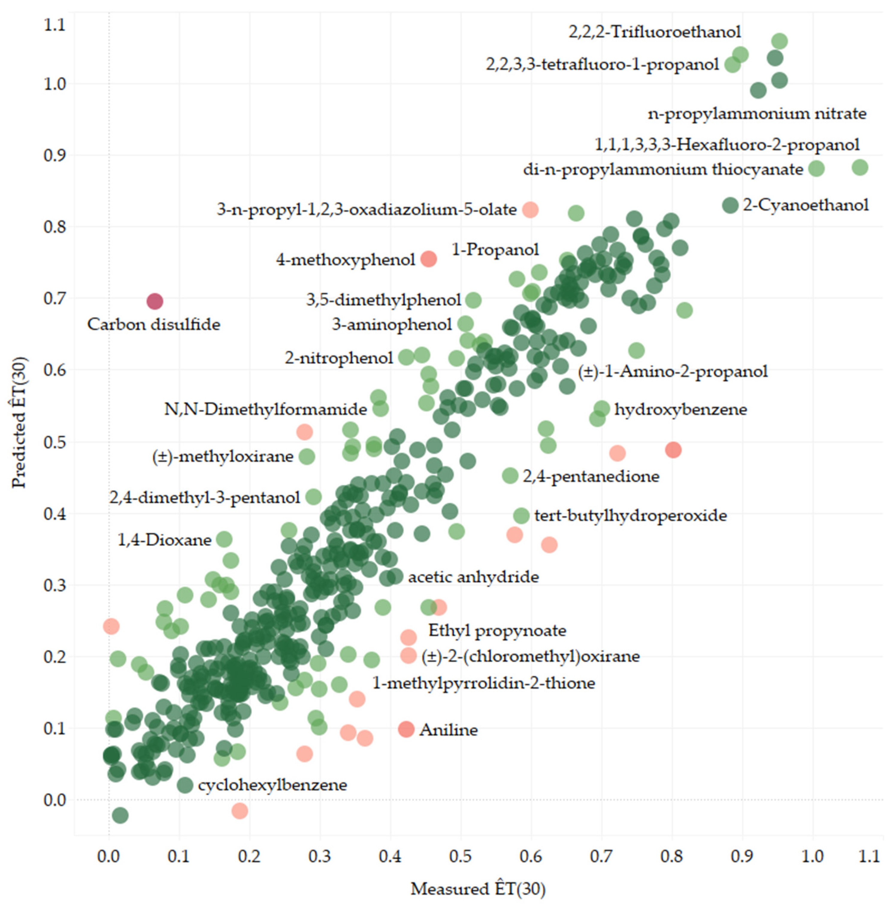
By fine-tuning a ChemBERTa-2 model on the largest subset of 461 solvents with unique SMILES and employing five-fold cross-validation, we created a transformer-based model that predicted Ê_T(30) values directly from the structure. The resulting model exhibited satisfactory performance, with the following test-set statistics: R² = 0.808, MAE = 0.071, RMSE = 0.099.

By employing SMILES enumeration [38], we achieved significant improvements in model performance, as evidenced by the test-set statistics calculated on the same dataset as before. Specifically, we calculated the test-set statistics from the measured and predicted Ê_T(30) values for the 461 original solvents using their original SMILES strings. The resulting test-set statistics were as follows: R² = 0.824, MAE = 0.066, RMSE = 0.095. The comparison between the measured and enhanced transformer-based model predicted Ê_T(30) values is illustrated in Figure 1.

To demonstrate its capabilities, we present the Ê_T(30) values predicted by Model 3 for several significant sustainable solvents sourced from Bradley et al. [24]. These solvents exhibit a range of Ê_T(30) values, including D-limonene (Ê_T(30) = 0.035), 2-methyltetrahydrofuran (Ê_T(30) = 0.163), cyclademol (Ê_T(30) = 0.244), oleic acid (Ê_T(30) = 0.342), geraniol (Ê_T(30) = 0.477), propionic acid (Ê_T(30) = 0.578), acetic acid (Ê_T(30) = 0.623), propylene glycol (Ê_T(30) = 0.761), and glycerol (Ê_T(30) = 0.815). It is evident that Model 3 is useful in predicting Ê_T(30) values and may be particularly valuable where direct measurement of Ê_T(30) values is difficult. See Table 1 for Model 3-predicted Ê_T(30) values for solvents with Abraham solvent coefficients but no experimentally determined Ê_T(30) values. This allows a comparison between the predictions of Model 2 and Model 3, highlighting the similarity in the obtained results and reinforcing the utility of Model 3.

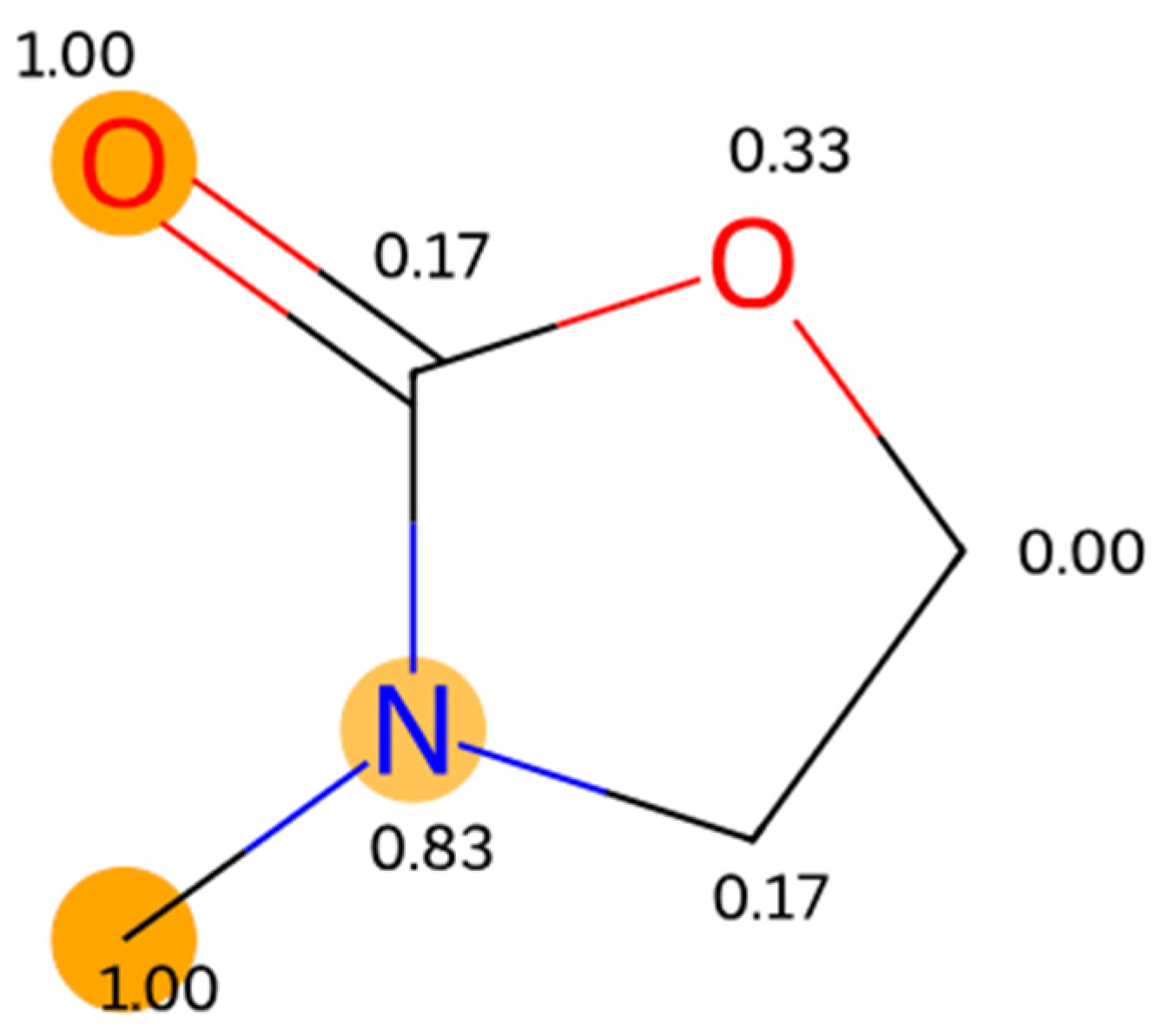
However, interpreting this model can be challenging because it does not rely on correlations with parameters that encode known chemical information. Some information can be gleaned by examining the attention mechanism of the model [41]. By analyzing the attention patterns, it is possible to gain insights into the model’s attentional priorities and understand which words (atoms) or phrases (functional groups) are deemed important for generating specific outputs, possibly discovering new chemistry, see Figure 2 for an example, selected at random.

The general analysis of the attention mechanism of Model 3 is beyond the scope of this paper, though we list it as an area of future research.

During the analysis of model outliers, it was observed that for Model 2, the three ionic liquids present in the modeling dataset ([BMIm]⁺ BF₄⁻, [BMIm]⁺ Tf₂N⁻, [BMIm]⁺ PF₆⁻) exhibited the highest absolute errors. These compounds demonstrated underpredicted Ê_T(30) values for Model 2, resulting in a mean absolute error of 0.152. It is worth mentioning that none of these ionic liquids possessed available ionic descriptors, which are likely crucial for achieving more accurate results.

In contrast, Model 3 exhibited a high level of accuracy in predicting the Ê_T(30) values for all three ionic liquids, as evidenced by a low mean absolute error of 0.051. However, an apparent failure of Model 3, illustrated in Figure 1, was observed in the case of carbon disulfide. In this instance, Model 3 significantly overpredicted the Ê_T(30) value, yielding a predicted value of 0.695 compared to the value of 0.065 collected from the literature, resulting in a substantial AE (absolute error) of 0.630. Conversely, Model 2 provided a more reasonable prediction for carbon disulfide, with an AE of 0.129. Model 2 had no significant outliers, likely due to its relatively small chemical space.

4. Discussion

The Abraham solvent parameter-based models, models 1 (s, a, b, j⁺, j⁻) and 2 (s, a, b), demonstrate strong predictive capabilities for compounds with measured Abraham solvent parameters. These models also exhibit good explanatory behavior regarding “solvent polarity,” as indicated by significant Abraham solvent descriptors such as s (encodes dipolarity/polarizability information) and descriptors a and b (which encode hydrogen-bond acidity/basicity related information). Test-set statistics support this observation, with Model 1 achieving an R² of 0.940, MAE of 0.037, and RMSE of 0.050 (N = 44), while Model 2 achieves an R² of 0.842, MAE of 0.085, and RMSE of 0.104 (N = 113).

These findings align with previous studies that have identified correlations between E_T(30) values and hydrogen-bond acidity/basicity and dipolarity/polarizability parameters on different scales, such as the Kamlet–Taft scale [21,22] and the Catalán scale [22,23]. Additionally, we note that other factors like electron lone pair interactions and volume-related dispersion forces, represented by the e and v parameters, respectively, do not significantly contribute to E_T(30) values.

Including ionic descriptors, j⁺ and j⁻, significantly improves the model’s performance, although it is essential to note that the chemical space of the sample is limited. Nonetheless, the poor performance of Model 2 in predicting E_T(30) values for ionic liquids (which lack available j⁺ and j⁻ descriptor values) underscores the importance of these descriptors in determining E_T(30) values in general.

Abraham solvent parameters also have the advantage over some other descriptor-based models in that they can be determined experimentally for most solvents (including mixtures, ionic liquids) and even predicted themselves for mono-solvents using standard machine learning techniques [24].

The optimized version of Model 3 exhibits strong predictive ability (R² = 0.824, MAE = 0.066, RMSE = 0.095). It stands out as the most versatile among all our models in that it can be applied to any solvent with an associated SMILES string, enhancing its practical utility.

The predictive applicability of Model 3 will prove useful, particularly in those organic solvents in which the betaine-30 dye has very limited solubility. The betaine-30 dye is insoluble in perfluorohydrocarbons, alkanes, aliphatic ethers, thioethers, amines, and esters having long alkyl chains. For these solvents, “experimental” E_T(30) values are often based on the absorption measurements of a lipophilic penta-tert-butyl substituted betaine dye, whose solvatochromic behavior is highly correlated with that of the betaine-30 zwitterionic molecule [30]. However, the interpretability of Model 3 poses challenges. In certain scenarios, it may produce significant errors, as observed with carbon disulfide, or give different predictions for molecules that exist in more than one tautomeric form. Further investigation should focus on analyzing the attention heads of Model 3, as this exploration may unveil new insights into chemistry and offer potential avenues for future research.

Finally, our use of an LLM is non-traditional and stands out in comparison to the standard linear techniques also used in the paper. Our LLM model is designed to seamlessly integrate into various workflows, adding a layer of abstraction that reduces the complexity for end-users. By leveraging ontology, our model benefits from a structured approach, enhancing its ability to understand, interpret, and generate predictions accurately. Agent assistance, on the other hand, enables the model to provide actionable insights and maintain interactive and dynamic communication with users. Knowledge engineering plays a crucial role in our model by facilitating the extraction, structuring, and analysis of domain-specific knowledge, enabling our model to make reliable predictions and offer a deeper understanding of the underlying chemical phenomena.