Quantifying the Risk Impact of Contextual Factors on Pedestrian Crash Outcomes in Data-Scarce Developing Country Settings
Abstract
1. Introduction
- Extracting trend data of contextual factors from literature sources.
- Generating a representative artificial dataset based on ranges and distributions reported in the literature, with outputs visualised as histograms and boxplots.
- External face validity checks of the generated data.
- Estimating the relative influence value (Fi) of each factor on crash frequency through pairwise correlation, stepwise regression, and transformation of regression coefficients.
- Performing sensitivity analysis and Fi uncertainty check.
- Mapping regression outputs with iRAP’s pedestrian crash risk framework to identify potential gaps.
2. Materials and Methods
2.1. Data Collection and Factor Selection
2.2. Extracting Trend Data of Each Factor from Literature Sources
2.3. Artificial Data Generation
- Using NumPy to generate 2000 random artificial data values for each variable. NumPy’s random number capabilities are widely used in scientific computing for simulation and statistical modelling tasks [14].
- To ensure statistical reliability, truncated normal distributions were applied on continuous variables to generate random numbers using SciPy’s truncnorm function [15]. This ensured that all values fall within the literature-derived minimum and maximum range while approximating the specified mean and standard deviation [16].
- Random binary distribution was used for categorical/binary variables based on the reported mean values. This is equivalent to a Bernoulli random distribution [17].
- The generated values were normalised and rescaled to have nearly the same mean and standard deviation using Pandas [18].
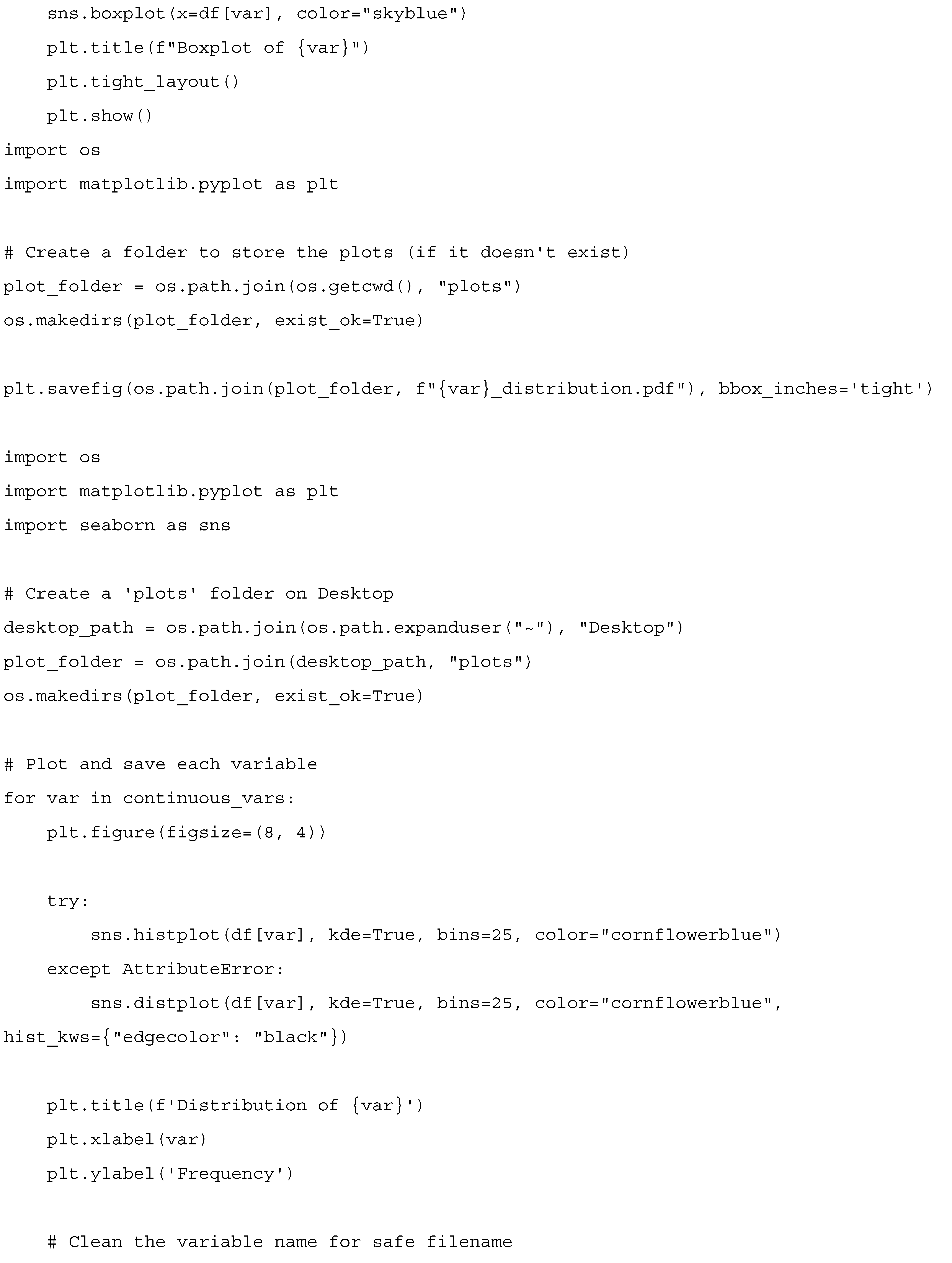
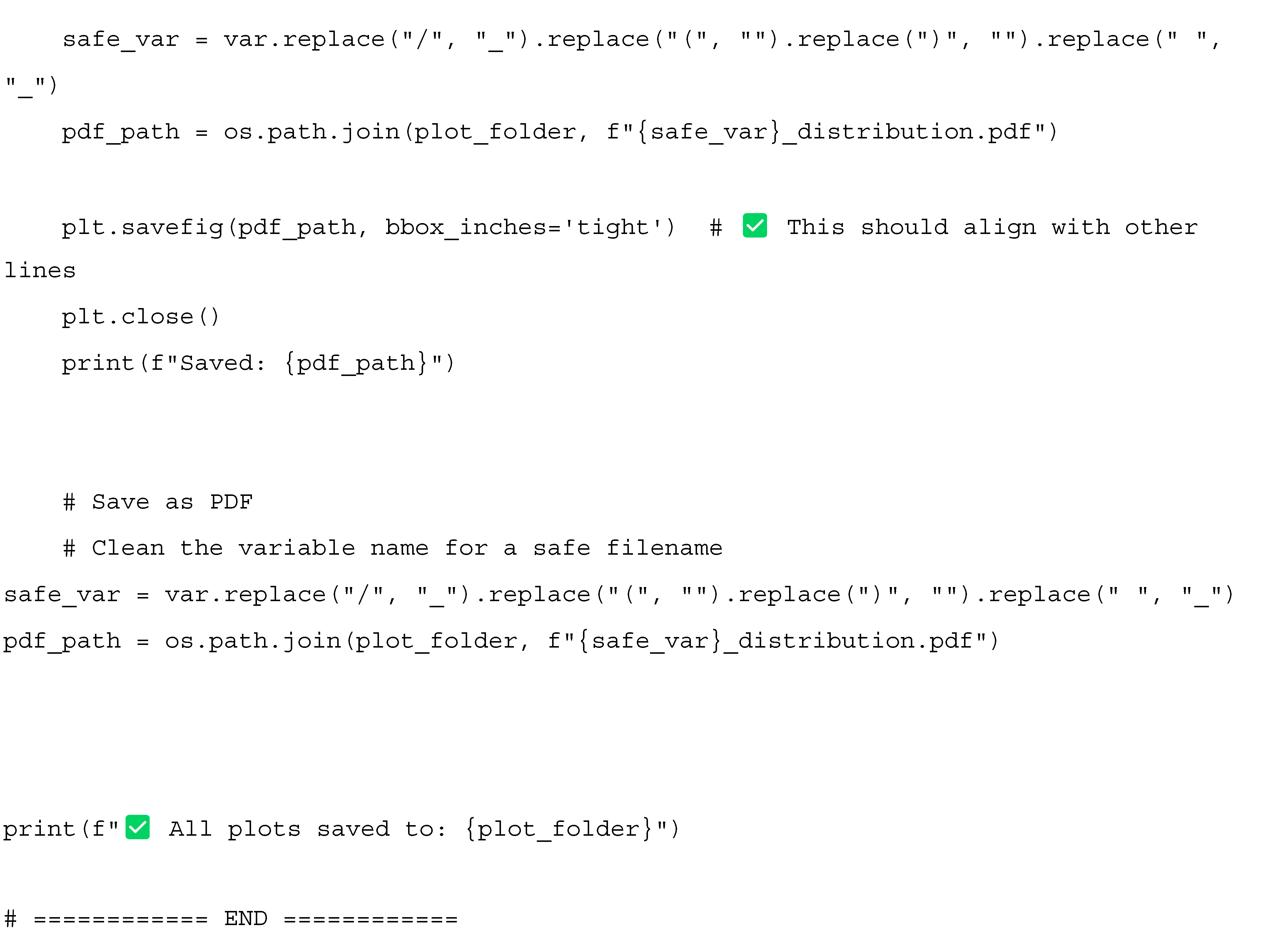
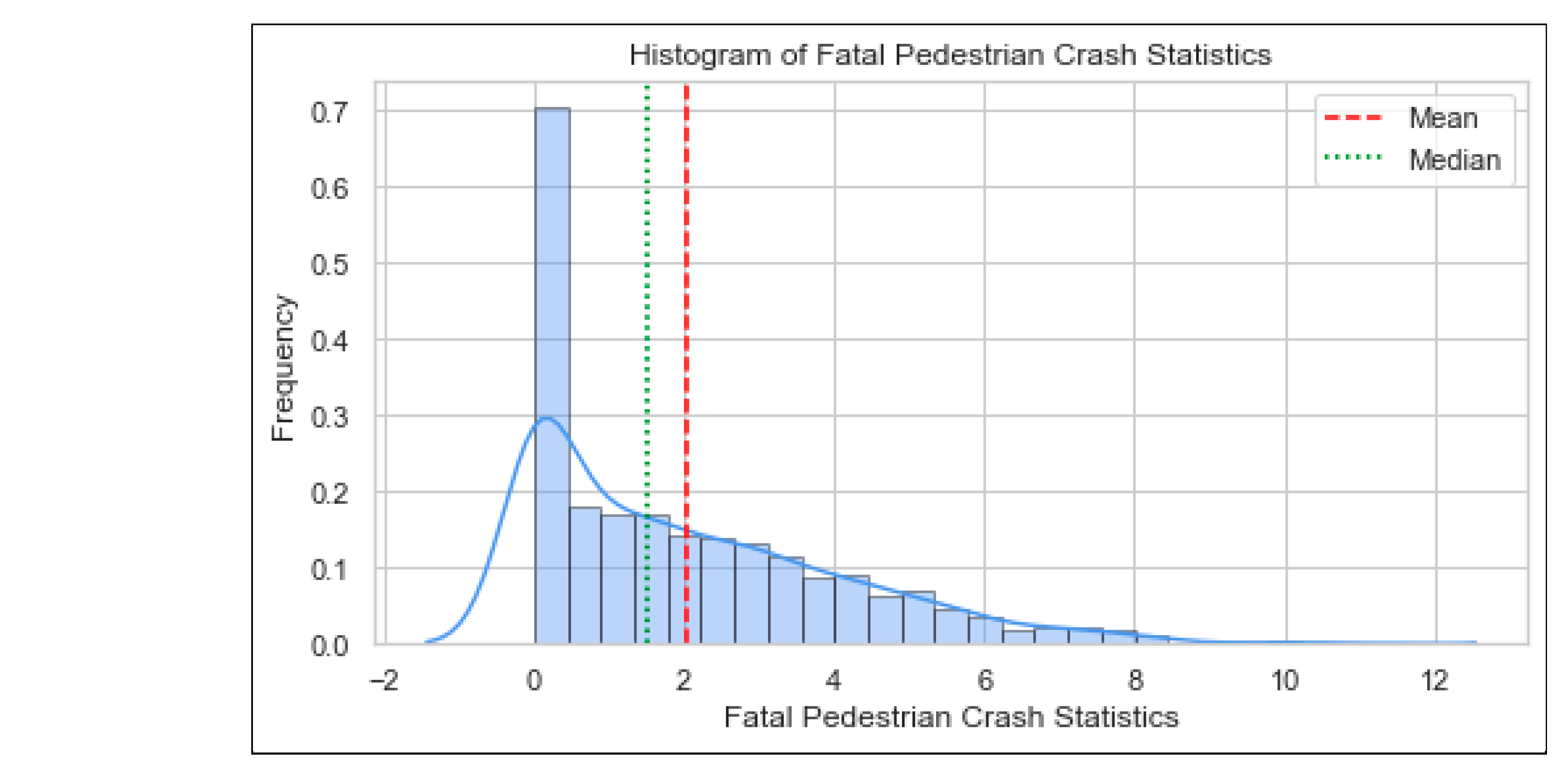
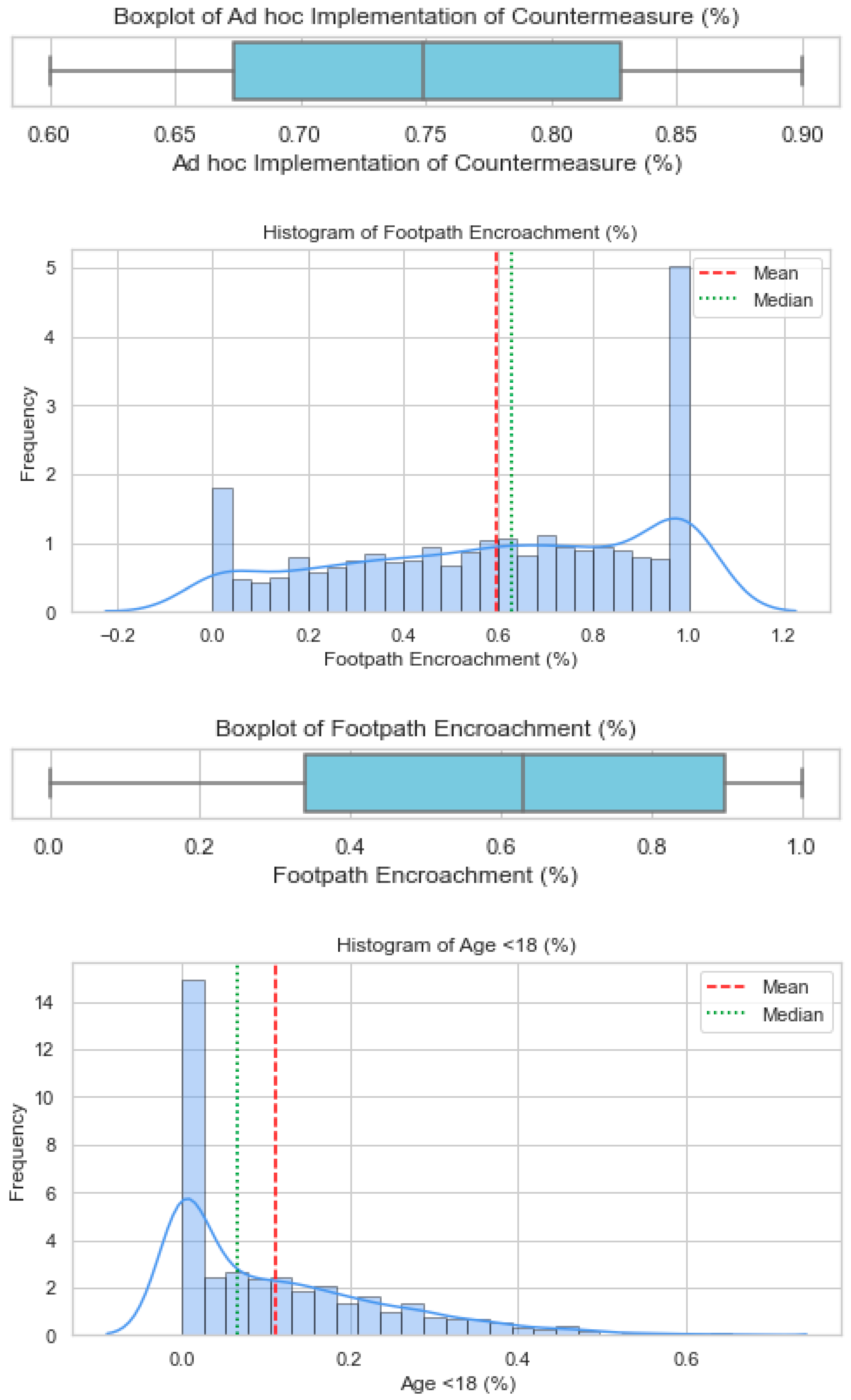
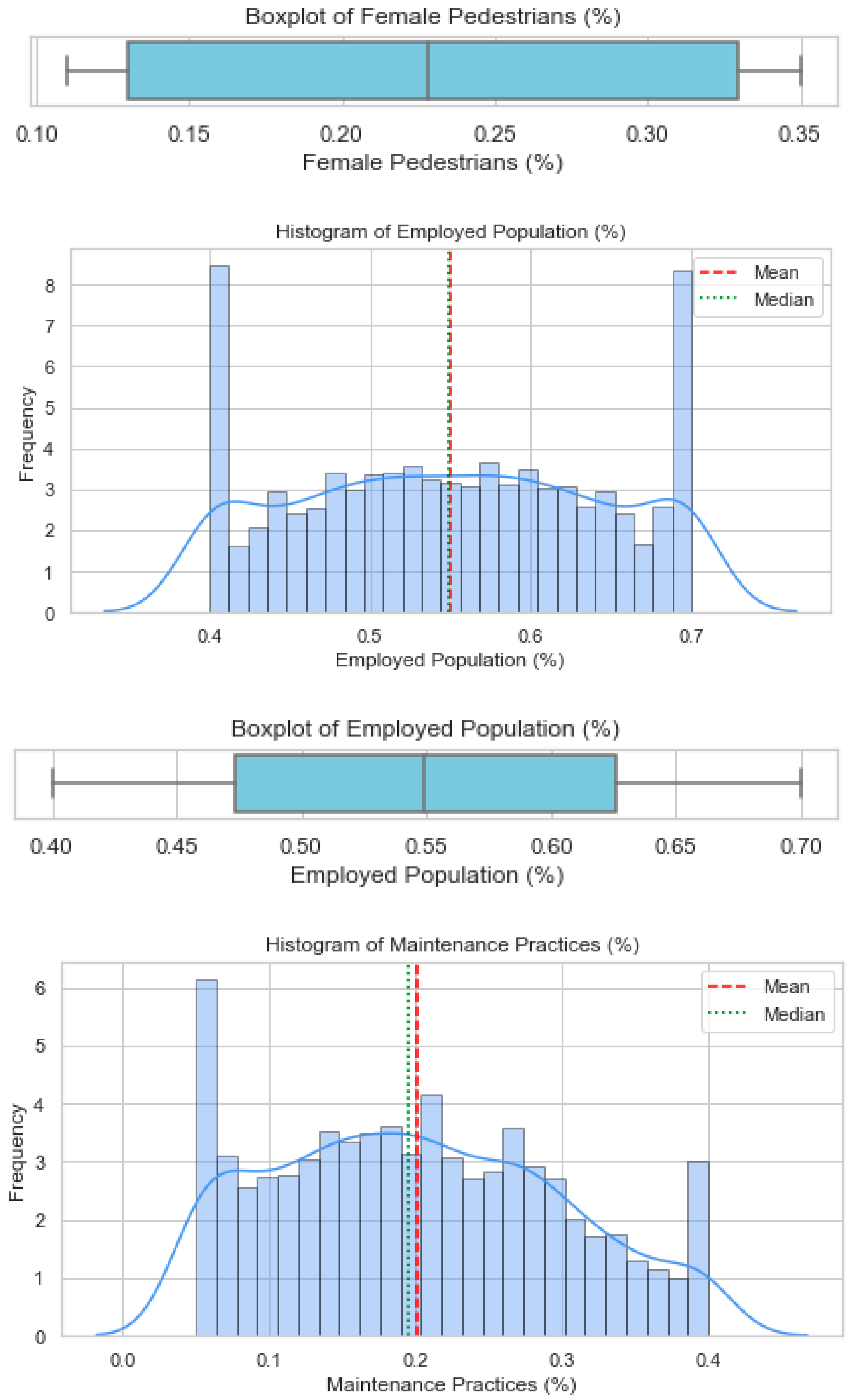
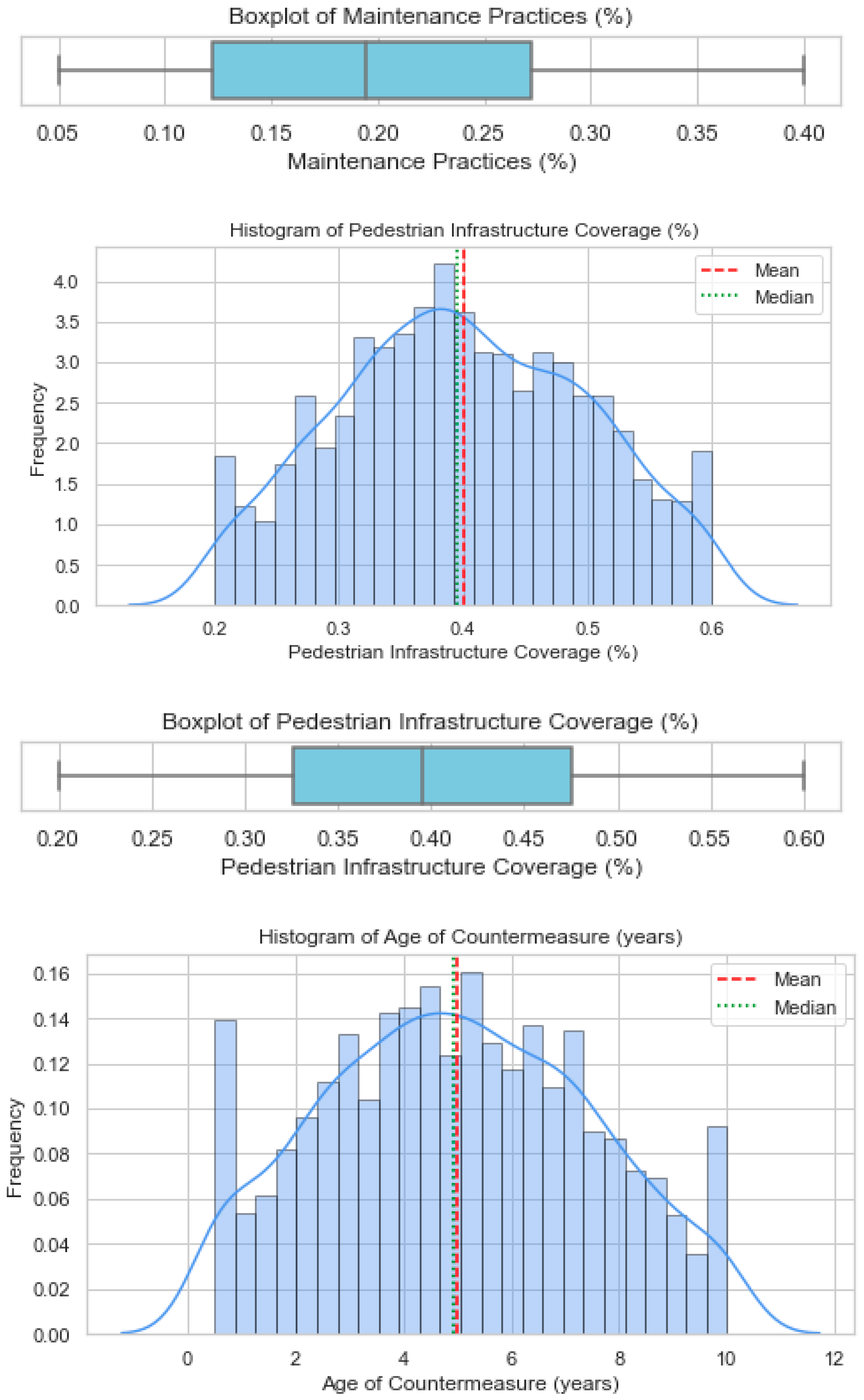
- Histograms and boxplots were generated using Matplotlib to visually verify variable distributions [19].
2.4. External Face Validity and Dependence of Generated Data
2.5. Estimating the Influence of Risk Factors on Pedestrian Crash Outcomes
2.5.1. Correlation Analyses
- Ranked the values of the independent variable (X) across all the 2000 random observations. Replaced each row value for the variable with their corresponding ranks.
- Ranked the fatal pedestrian crash counts/dependent variable (Y) across 2000 random observations.
- Calculated the Spearman’s correlation coefficient between the two ranked pairs of variables using the following correlation formula:
- ρ is the Spearman correlation coefficient;
- di is the difference in ranks between the two variables (e.g., di = rank(Xi)—rank(Yi));
- n is the number of observations (where n = 2000).
2.5.2. Stepwise Regression Modelling
- Model 1: Constant only (baseline);
- Model 2: Traffic exposure and operational variables (e.g., mixed traffic conditions);
- Model 3: Land use and planning variables (e.g., road use);
- Model 4: Demographics (e.g., age group);
- Model 5: Infrastructure and roadway variables (e.g., coverage of pedestrian infrastructure);
- Model 6: Full model (combined all variables).
- yi is the expected number of crashes/crash count at point i.
- X1i, X2i, ….: independent/predictor variables.
- β0, β2, …: coefficients estimated by maximum likelihood.
- Restricted log-likelihood () of the null (intercept-only) model;
- McFadden’s Pseudo-R2 static/log-likelihood ratio index (ρ2) given by:
- Akaike Information Criterion (AIC), which is given as:
2.5.3. Transforming NB Coefficients into Risk Factor Influence Values (Fi)
2.6. Sensitivity Analysis and Fi Uncertainty
- Bootstrap resampling: 1000 bootstrap samples of the synthetic dataset were drawn with replacement. For each bootstrap, negative binomial (NB) models were re-estimated and Fi values recalculated. This allowed the derivation of 95% confidence intervals.
- Scenario perturbation: The synthetic dataset was resampled under varying sample sizes (n = 1000; 2000; 5000) and with multiplicative noise applied to predictor variables (5% and 10%). For each scenario, Fi values were recalculated, and stability of variable rankings was assessed using Kendall’s τ correlation with baseline rankings.
2.7. Comparative Analyses (Mapping of Factors to NB Model and iRAP Framework)
| Characteristics | Variables | Variable Type | Minimum | Maximum | Mean (μ) | Standard Deviation (δ) | References | Country |
|---|---|---|---|---|---|---|---|---|
| Safety Performance | Fatal Pedestrian Crash Statistics | Continuous | 0.00 | 13.00 | 1.83 | 2.29 | [10] | India |
| Traffic Exposures and Operational Characteristics | Log (Average Daily Traffic Volume) | Continous | 4.24 | 5.47 | 4.71 | 0.22 | [10] | India |
| Log (Average Daily Pedestrian Volume) | Continuous | 3.33 | 5.25 | 4.58 | 0.35 | [10] | India | |
| Speed (km/h) | Continuous | 30.00 | 65.00 | 42.48 | 9.38 | [10] | India | |
| Pedestrian to Vehicle Volume Ratio/Mixed Traffic Conditions | Continuous | 0.05 | 9.20 | 1.09 | 1.23 | [10] | India | |
| Vehicle age/technology (%) | Continuous | 0.50 | 0.90 | 0.70 | 0.13 | [29] | Nigeria, Ghana, Ethiopia, Kenya | |
| Compliance/Presence of Overtaking Tendency of Vehicle (1/0) | Categorical | 0.00 | 1.00 | 0.67 | 0.48 | [10] | India | |
| Enforcement of Traffic rules (Yes = 1; No = 0) | Categorical | 0.00 | 1.00 | 0.50 | 0.50 | [10,30] | India | |
| Public safety awareness level (%) | Continuous | 0.31 | 0.68 | 0.50 | 0.13 | [31] | Bangladesh | |
| Driver safety awareness level (%) | Continuous | 0.38 | 0.54 | 0.48 | 0.13 | [32] | Quatar | |
| Time of the Day (visibility) (1/0) | Categorical | 0.00 | 1.00 | 0.49 | 0.50 | [33] | India | |
| Land use and Planning | Hierarchical Road Classification/Road Use (%) | Continuous | 0.16 | 0.80 | 0.45 | 0.20 | [34] | Brazil, Columbia, Tanzania |
| Design Configuration (%) | Continuous | 0.10 | 0.55 | 0.30 | 0.15 | [35,36,37] | Ethiopia, India | |
| Ad hoc implementation of countermeasures (%) | Continuous | 0.60 | 0.90 | 0.75 | 0.10 | [38,39,40,41] | Uganda, India, Ghana | |
| Encroachment of Footpath by Street vendors (%) | Continuous | 0.00 | 1.00 | 0.61 | 0.36 | [10] | India | |
| Human Capacity of responsible agencies (Adequate = 1, Poor = 0) | Categorical | 0.00 | 1.00 | 0.50 | 0.30 | [42] | World Bank | |
| Demographics | Age group (%) | Below 18 years (%) | 0.00 | 0.90 | 0.09 | 0.15 | [33] | India |
| 18–49 years (in %) | 0.06 | 1.00 | 0.79 | 0.15 | [33] | India | ||
| 50+ years (%) | 0.00 | 0.33 | 0.11 | 0.07 | [33] | India | ||
| Gender (%) | Male pedestrians (%) | 0.02 | 0.90 | 0.73 | 0.15 | [33] | India | |
| Female (%) | 0.11 | 0.35 | 0.23 | 0.12 | [43] | USA | ||
| Employed population (%) | Continuous | 0.40 | 0.70 | 0.55 | 0.10 | [44] | World Bank | |
| Infrastructure and Roadway Factors | Maintenance Practices/level (%) | Continuous | 0.05 | 0.40 | 0.20 | 0.10 | [35,36] | Ghana and Ethiopia |
| Coverage of pedestrian infrastructure (%) | Continuous | 0.20 | 0.60 | 0.40 | 0.10 | [41] | India | |
| Vandalism of Street Furniture (Never = 1; Sometimes = 0.5; Always = 0) | Categorical | 0.00 | 1.00 | 0.70 | 0.20 | [45] | Turkey | |
| Age of the countermeasure (years) | Continuous | 0.50 | 10.00 | 5.00 | 2.50 | [46] | USA | |
| Appropriate location of countermeasure (1/0) | Categorical | 0.00 | 1.00 | 0.60 | 0.20 | [37] | Ethiopia |
| Characteristics | Variables | Variable Type | Minimum | Maximum | Mean (μ) | Median | Standard Deviation (δ) | StdErr | 95% CI Lower Bound | 95% CI Upper Bound |
|---|---|---|---|---|---|---|---|---|---|---|
| Safety Performance | Fatal Pedestrian Crash Statistics | Continuous | 0.00 | 10.67 | 2.03 | 1.50 | 2.06 | 0.05 | 1.94 | 2.12 |
| Traffic Exposures and Operational Characteristics | Log (Average Daily Traffic Volume) | Continuous | 4.24 | 5.47 | 4.71 | 4.71 | 0.22 | 0.00 | 4.70 | 4.72 |
| Log (Average Daily Pedestrian Volume) | Continuous | 3.37 | 5.25 | 4.58 | 4.59 | 0.35 | 0.01 | 4.56 | 4.59 | |
| Speed (km/h) | Continuous | 30.00 | 65.00 | 42.67 | 42.00 | 9.06 | 0.20 | 42.27 | 43.06 | |
| Pedestrian to Vehicle Volume Ratio/Mixed Traffic Conditions | Continuous | 0.05 | 6.07 | 1.19 | 0.95 | 1.11 | 0.02 | 1.14 | 1.24 | |
| Vehicle age/technology (%) | Continuous | 0.50 | 0.90 | 0.70 | 0.70 | 0.12 | 0.00 | 0.69 | 0.71 | |
| Compliance/Presence of Overtaking Tendency of Vehicle (1/0) | Categorical | 0.00 | 1.00 | 0.66 | 1.00 | 0.48 | 0.01 | 0.63 | 0.68 | |
| Enforcement of Traffic rules (Yes = 1; No = 0) | Categorical | 0.00 | 1.00 | 0.51 | 1.00 | 0.50 | 0.01 | 0.48 | 0.53 | |
| Public safety awareness level (%) | Continuous | 0.31 | 0.68 | 0.50 | 0.50 | 0.12 | 0.00 | 0.49 | 0.51 | |
| Driver safety awareness level (%) | Continuous | 0.38 | 0.54 | 0.47 | 0.49 | 0.07 | 0.00 | 0.47 | 0.47 | |
| Time of the Day (visibility) (1/0) | Categorical | 0.00 | 1.00 | 0.48 | 0.00 | 0.50 | 0.01 | 0.46 | 0.50 | |
| Land use and Planning | Hierarchical Road Classification/Road Use (%) | Continuous | 0.16 | 0.80 | 0.45 | 0.44 | 0.19 | 0.00 | 0.44 | 0.46 |
| Design Configuration (%) | Continuous | 0.10 | 0.55 | 0.30 | 0.29 | 0.14 | 0.00 | 0.30 | 0.31 | |
| Ad hoc implementation of countermeasures (%) | Continuous | 0.60 | 0.90 | 0.75 | 0.75 | 0.09 | 0.00 | 0.75 | 0.75 | |
| Encroachment of Footpath by Street vendors (%) | Continuous | 0.00 | 1.00 | 0.60 | 0.64 | 0.32 | 0.01 | 0.58 | 0.61 | |
| Human Capacity of responsible agencies (Adequate = 1, Poor = 0) | Categorical | 0.00 | 1.00 | 0.50 | 0.00 | 0.50 | 0.01 | 0.48 | 0.52 | |
| Demographics | Age group (%) | Below 18 years (%) | 0.00 | 0.69 | 0.11 | 0.07 | 0.13 | 0.00 | 0.10 | 0.12 |
| 18–49 years (in %) | 0.21 | 1.00 | 0.79 | 0.80 | 0.15 | 0.00 | 0.78 | 0.79 | ||
| 50+ years (%) | 0.00 | 0.33 | 0.11 | 0.10 | 0.07 | 0.00 | 0.11 | 0.11 | ||
| Gender (%) | Male pedestrians (%) | 0.13 | 0.90 | 0.72 | 0.74 | 0.14 | 0.00 | 0.72 | 0.73 | |
| Female (%) | 0.11 | 0.35 | 0.23 | 0.23 | 0.09 | 0.00 | 0.23 | 0.23 | ||
| Employed population (%) | Continuous | 0.40 | 0.70 | 0.55 | 0.55 | 0.09 | 0.00 | 0.55 | 0.55 | |
| Infrastructure and Roadway Factors | Maintenance Practices/level (%) | Continuous | 0.05 | 0.40 | 0.20 | 0.20 | 0.10 | 0.00 | 0.20 | 0.21 |
| Coverage of pedestrian infrastructure (%) | Continuous | 0.20 | 0.60 | 0.40 | 0.40 | 0.10 | 0.00 | 0.40 | 0.40 | |
| Vandalism of Street Furniture (Never = 1; Sometimes = 0.5; Always = 0) | Categorical | 0.00 | 1.00 | 0.70 | 1.00 | 0.46 | 0.01 | 0.68 | 0.72 | |
| Age of the countermeasure (years) | Continuous | 0.50 | 10.00 | 5.01 | 5.04 | 2.47 | 0.06 | 4.90 | 5.12 | |
| Appropriate location of countermeasure (1/0) | Categorical | 0.00 | 1.00 | 0.61 | 1.00 | 0.49 | 0.01 | 0.59 | 0.63 |
| Variable | Min | Max | Mean | Std Dev | Spearman Rho | T-Statistic | p-Value |
|---|---|---|---|---|---|---|---|
| Log Average Daily Traffic Volume | 4.240 | 5.470 | 4.710 | 0.220 | −0.029 | −1.285 | 0.199 |
| Log Average Daily Pedestrian Volume | 3.364 | 5.250 | 4.580 | 0.349 | 0.030 | 1.336 | 0.182 |
| Speed (km/h) | 30.000 | 65.000 | 42.697 | 8.988 | 0.029 | 1.282 | 0.200 |
| Pedestrian to Vehicle Volume Ratio | 0.050 | 6.087 | 1.179 | 1.128 | 0.000 | 0.010 | 0.992 |
| Vehicle age technology (%) | 0.500 | 0.900 | 0.700 | 0.122 | 0.003 | 0.124 | 0.901 |
| Overtaking Tendency (1/0) | 0.000 | 1.000 | 0.668 | 0.471 | −0.037 | −1.662 | 0.097 |
| Traffic Rule Enforcement (1/0) | 0.000 | 1.000 | 0.517 | 0.500 | 0.009 | 0.387 | 0.699 |
| Public Safety Awareness (%) | 0.310 | 0.680 | 0.499 | 0.119 | −0.026 | −1.161 | 0.246 |
| Driver Safety Awareness (%) | 0.380 | 0.540 | 0.468 | 0.069 | 0.017 | 0.755 | 0.450 |
| Time of Day Visibility (1/0) | 0.000 | 1.000 | 0.491 | 0.500 | 0.011 | 0.490 | 0.624 |
| Road Use (%) | 0.160 | 0.800 | 0.452 | 0.191 | 0.001 | 0.039 | 0.969 |
| Design Configuration (%) | 0.100 | 0.550 | 0.302 | 0.139 | 0.018 | 0.791 | 0.429 |
| Ad hoc implementation of countermeasures (%) | 0.600 | 0.900 | 0.751 | 0.094 | −0.032 | −1.407 | 0.160 |
| Footpath Encroachment (%) | 0.000 | 1.000 | 0.596 | 0.326 | 0.008 | 0.342 | 0.733 |
| Human Capacity of Agencies (1/0) | 0.000 | 1.000 | 0.498 | 0.500 | 0.013 | 0.581 | 0.562 |
| Age < 18 (%) | 0.000 | 0.685 | 0.111 | 0.128 | −0.021 | −0.926 | 0.355 |
| Age 18–49 (%) | 0.181 | 1.000 | 0.788 | 0.147 | 0.031 | 1.373 | 0.170 |
| Age 50+ (%) | 0.000 | 0.330 | 0.111 | 0.069 | −0.011 | −0.487 | 0.627 |
| Male Pedestrians (%) | 0.158 | 0.900 | 0.725 | 0.143 | 0.036 | 1.616 | 0.106 |
| Female Pedestrians (%) | 0.110 | 0.350 | 0.230 | 0.092 | −0.023 | −1.016 | 0.310 |
| Employed Population (%) | 0.400 | 0.700 | 0.550 | 0.094 | 0.021 | 0.947 | 0.344 |
| Maintenance Practices (%) | 0.050 | 0.400 | 0.201 | 0.097 | −0.006 | −0.251 | 0.802 |
| Pedestrian Infrastructure Coverage (%) | 0.200 | 0.600 | 0.400 | 0.099 | 0.008 | 0.374 | 0.709 |
| Street Furniture Vandalism (0/0.5/1) | 0.000 | 1.000 | 0.680 | 0.467 | −0.024 | −1.074 | 0.283 |
| Age of Countermeasure years | 0.500 | 10.000 | 5.006 | 2.466 | −0.022 | −0.968 | 0.333 |
| Appropriate Countermeasure Location (1/0) | 0.000 | 1.000 | 0.608 | 0.488 | 0.033 | 1.468 | 0.142 |
| FT | T | P | S | R | VAT | OT | TR | PSA | DSA | TD | RU | DC | CA | FE | HCA | AG1 | AG2 | AG3 | MP | FP | EP | MTP | PIC | SFV | AC | ACL | |
|---|---|---|---|---|---|---|---|---|---|---|---|---|---|---|---|---|---|---|---|---|---|---|---|---|---|---|---|
| FT | 1.000 | ||||||||||||||||||||||||||
| T | −0.029 | 1.000 | |||||||||||||||||||||||||
| P | 0.030 | 0.004 | 1.000 | ||||||||||||||||||||||||
| S | 0.029 | −0.021 | −0.019 | 1.000 | |||||||||||||||||||||||
| R | 0.000 | −0.038 | 0.005 | 0.017 | 1.000 | ||||||||||||||||||||||
| VAT | 0.003 | −0.005 | 0.013 | −0.013 | −0.033 | 1.000 | |||||||||||||||||||||
| OT | −0.037 | 0.017 | −0.001 | −0.023 | −0.011 | 0.018 | 1.000 | ||||||||||||||||||||
| TR | 0.009 | 0.003 | −0.075 | 0.019 | −0.030 | −0.034 | 0.009 | 1.000 | |||||||||||||||||||
| PSA | −0.026 | 0.025 | −0.002 | 0.018 | 0.019 | −0.039 | 0.063 | 0.006 | 1.000 | ||||||||||||||||||
| DSA | 0.017 | 0.031 | 0.013 | 0.003 | 0.004 | −0.001 | 0.003 | −0.025 | 0.006 | 1.000 | |||||||||||||||||
| TD | 0.011 | 0.012 | −0.007 | 0.001 | 0.018 | 0.024 | 0.054 | −0.016 | 0.007 | −0.005 | 1.000 | ||||||||||||||||
| RU | 0.001 | 0.001 | −0.016 | 0.018 | 0.025 | 0.016 | −0.013 | 0.015 | 0.015 | 0.021 | −0.017 | 1.000 | |||||||||||||||
| DC | 0.018 | 0.017 | 0.004 | −0.003 | −0.003 | −0.028 | −0.009 | 0.002 | 0.004 | −0.013 | −0.020 | 0.014 | 1.000 | ||||||||||||||
| CA | −0.031 | 0.026 | −0.005 | −0.024 | 0.011 | 0.001 | 0.021 | −0.047 | 0.011 | 0.000 | 0.001 | 0.017 | −0.025 | 1.000 | |||||||||||||
| FE | 0.008 | −0.011 | −0.017 | 0.017 | 0.012 | 0.000 | 0.009 | −0.003 | −0.023 | 0.027 | 0.018 | 0.011 | 0.022 | 0.056 | 1.000 | ||||||||||||
| HCA | 0.013 | −0.006 | 0.034 | 0.033 | 0.021 | 0.019 | −0.011 | −0.008 | −0.009 | 0.004 | 0.005 | 0.025 | −0.008 | 0.009 | −0.009 | 1.000 | |||||||||||
| AG1 | −0.021 | 0.015 | −0.004 | 0.009 | −0.035 | −0.017 | −0.002 | −0.027 | 0.025 | 0.005 | −0.031 | 0.022 | 0.019 | 0.007 | 0.032 | −0.056 | 1.000 | ||||||||||
| AG2 | 0.031 | −0.025 | 0.025 | −0.010 | −0.003 | −0.014 | 0.002 | 0.029 | −0.007 | −0.001 | −0.001 | 0.019 | 0.003 | −0.021 | −0.029 | 0.017 | −0.017 | 1.000 | |||||||||
| AG3 | −0.011 | 0.012 | 0.004 | 0.010 | 0.023 | 0.023 | 0.019 | −0.043 | −0.013 | 0.008 | 0.027 | −0.002 | 0.008 | 0.021 | −0.008 | −0.004 | −0.022 | 0.033 | 1.000 | ||||||||
| MP | 0.036 | 0.005 | −0.002 | 0.011 | −0.027 | 0.020 | 0.070 | −0.021 | 0.019 | 0.036 | −0.036 | −0.015 | −0.035 | 0.026 | −0.004 | 0.005 | −0.003 | 0.025 | 0.043 | 1.000 | |||||||
| FP | −0.023 | 0.018 | −0.012 | −0.022 | 0.012 | 0.009 | −0.002 | −0.001 | 0.010 | 0.043 | −0.013 | −0.023 | 0.014 | −0.022 | 0.012 | −0.006 | 0.018 | 0.021 | −0.019 | 0.008 | 1.000 | ||||||
| EP | 0.021 | −0.017 | 0.030 | −0.005 | 0.012 | −0.021 | 0.016 | −0.020 | 0.018 | 0.008 | −0.002 | 0.015 | −0.009 | 0.002 | 0.007 | −0.005 | −0.058 | 0.026 | 0.001 | 0.013 | −0.017 | 1.000 | |||||
| MTP | −0.006 | −0.038 | −0.008 | −0.013 | 0.013 | −0.025 | −0.003 | −0.004 | 0.011 | 0.014 | 0.025 | 0.003 | −0.007 | 0.013 | −0.003 | 0.029 | 0.043 | −0.007 | −0.006 | 0.015 | −0.057 | 0.023 | 1.000 | ||||
| PIC | 0.008 | −0.012 | −0.043 | 0.012 | −0.040 | −0.019 | 0.008 | −0.038 | −0.045 | 0.029 | 0.001 | 0.013 | −0.004 | 0.003 | −0.002 | 0.023 | −0.007 | 0.019 | −0.036 | 0.012 | −0.052 | 0.021 | 0.022 | 1.000 | |||
| SFV | −0.024 | 0.054 | 0.001 | −0.018 | 0.020 | −0.004 | −0.034 | −0.019 | −0.026 | −0.040 | 0.027 | 0.010 | 0.003 | −0.007 | 0.011 | 0.030 | −0.005 | −0.023 | −0.008 | −0.026 | 0.016 | −0.013 | 0.001 | 0.009 | 1.000 | ||
| AC | −0.022 | −0.009 | −0.013 | 0.021 | −0.019 | −0.038 | 0.003 | −0.029 | −0.001 | −0.024 | 0.015 | −0.038 | 0.009 | 0.019 | 0.006 | −0.001 | −0.017 | −0.002 | −0.021 | 0.032 | −0.009 | 0.048 | −0.001 | −0.021 | −0.007 | 1.000 |
| Coefficient (β) | StdErr | z-Value | P > |z| | CI Lower | CI Upper | Variable | Model |
|---|---|---|---|---|---|---|---|
| 0.704 | 0.027 | 25.750 | 0.000 | 0.650 | 0.758 | intercept | Model_1_Baseline |
| 0.680 | 0.720 | 0.943 | 0.345 | −0.732 | 2.092 | const | Model_2_Traffic |
| −0.146 | 0.125 | −1.174 | 0.240 | −0.391 | 0.098 | Log Average Daily Traffic Volume | Model_2_Traffic |
| 0.109 | 0.078 | 1.393 | 0.164 | −0.045 | 0.263 | Log Average Daily Pedestrian Volume | Model_2_Traffic |
| 0.003 | 0.003 | 0.832 | 0.405 | −0.003 | 0.008 | Speed (km/h) | Model_2_Traffic |
| 0.004 | 0.024 | 0.150 | 0.881 | −0.044 | 0.051 | Pedestrian to Vehicle Volume Ratio | Model_2_Traffic |
| 0.142 | 0.224 | 0.635 | 0.526 | −0.296 | 0.580 | Vehicle age technology (%) | Model_2_Traffic |
| 1.018 | 0.239 | 4.262 | 0.000 | 0.550 | 1.486 | const | Model_3_Land_Use |
| 0.060 | 0.143 | 0.416 | 0.677 | −0.221 | 0.340 | Road Use (%) | Model_3_Land_Use |
| 0.112 | 0.196 | 0.569 | 0.569 | −0.273 | 0.497 | Design Configuration (%) | Model_3_Land_Use |
| −0.496 | 0.291 | −1.707 | 0.088 | −1.066 | 0.073 | Ad hoc implementation of countermeasures (%) | Model_3_Land_Use |
| −0.005 | 0.084 | −0.065 | 0.948 | −0.170 | 0.159 | Footpath Encroachment (%) | Model_3_Land_Use |
| 0.446 | 0.267 | 1.666 | 0.096 | −0.078 | 0.970 | const | Model_4_Demographic |
| 0.065 | 0.214 | 0.302 | 0.763 | −0.355 | 0.484 | Age < 18 (%) | Model_4_Demographic |
| 0.154 | 0.186 | 0.826 | 0.409 | −0.212 | 0.519 | Age 18–49 (%) | Model_4_Demographic |
| −0.073 | 0.398 | −0.183 | 0.854 | −0.852 | 0.706 | Age 50+ (%) | Model_4_Demographic |
| 0.088 | 0.192 | 0.460 | 0.645 | −0.288 | 0.464 | Male Pedestrians (%) | Model_4_Demographic |
| −0.140 | 0.298 | −0.468 | 0.639 | −0.724 | 0.445 | Female Pedestrians (%) | Model_4_Demographic |
| 0.191 | 0.292 | 0.655 | 0.512 | −0.381 | 0.764 | Employed Population (%) | Model_4_Demographic |
| 0.741 | 0.149 | 4.972 | 0.000 | 0.449 | 1.033 | const | Model_5_Infrastructure |
| −0.100 | 0.283 | −0.354 | 0.723 | −0.654 | 0.454 | Maintenance Practices (%) | Model_5_Infrastructure |
| 0.077 | 0.277 | 0.277 | 0.782 | −0.466 | 0.620 | Pedestrian Infrastructure Coverage (%) | Model_5_Infrastructure |
| −0.032 | 0.058 | −0.553 | 0.581 | −0.147 | 0.082 | Street Furniture Vandalism (0/0.5/1) | Model_5_Infrastructure |
| −0.011 | 0.011 | −0.961 | 0.336 | −0.032 | 0.011 | Age of Countermeasure (years) | Model_5_Infrastructure |
| 0.045 | 0.056 | 0.799 | 0.424 | −0.065 | 0.155 | Appropriate Countermeasure Location (1/0) | Model_5_Infrastructure |
| 0.765 | 0.819 | 0.934 | 0.350 | −0.840 | 2.369 | const | Model_6_Full |
| −0.145 | 0.125 | −1.159 | 0.247 | −0.391 | 0.100 | Log Average Daily Traffic Volume | Model_6_Full |
| 0.103 | 0.079 | 1.310 | 0.190 | −0.051 | 0.257 | Log Average Daily Pedestrian Volume | Model_6_Full |
| 0.002 | 0.003 | 0.802 | 0.423 | −0.004 | 0.008 | Speed (km/h) | Model_6_Full |
| 0.004 | 0.024 | 0.177 | 0.860 | −0.043 | 0.052 | Pedestrian to Vehicle Volume Ratio | Model_6_Full |
| 0.149 | 0.225 | 0.663 | 0.507 | −0.291 | 0.589 | Vehicle age technology (%) | Model_6_Full |
| 0.049 | 0.144 | 0.344 | 0.731 | −0.232 | 0.331 | Road Use (%) | Model_6_Full |
| 0.126 | 0.197 | 0.640 | 0.522 | −0.260 | 0.512 | Design Configuration (%) | Model_6_Full |
| −0.460 | 0.292 | −1.578 | 0.114 | −1.031 | 0.111 | Ad hoc implementation of countermeasures (%) | Model_6_Full |
| 0.000 | 0.084 | 0.002 | 0.998 | −0.165 | 0.165 | Footpath Encroachment (%) | Model_6_Full |
| 0.057 | 0.215 | 0.264 | 0.792 | −0.365 | 0.478 | Age < 18 (%) | Model_6_Full |
| 0.135 | 0.187 | 0.725 | 0.469 | −0.231 | 0.502 | Age 18–49 (%) | Model_6_Full |
| −0.083 | 0.399 | −0.208 | 0.835 | −0.864 | 0.698 | Age 50+ (%) | Model_6_Full |
| 0.109 | 0.193 | 0.568 | 0.570 | −0.268 | 0.487 | Male Pedestrians (%) | Model_6_Full |
| −0.152 | 0.300 | −0.507 | 0.612 | −0.740 | 0.436 | Female Pedestrians (%) | Model_6_Full |
| 0.203 | 0.293 | 0.691 | 0.490 | −0.372 | 0.777 | Employed Population (%) | Model_6_Full |
| −0.116 | 0.284 | −0.408 | 0.683 | −0.672 | 0.441 | Maintenance Practices (%) | Model_6_Full |
| 0.056 | 0.279 | 0.202 | 0.840 | −0.490 | 0.603 | Pedestrian Infrastructure Coverage (%) | Model_6_Full |
| −0.026 | 0.059 | −0.447 | 0.655 | −0.141 | 0.089 | Street Furniture Vandalism (0/0.5/1) | Model_6_Full |
| −0.010 | 0.011 | −0.920 | 0.358 | −0.032 | 0.012 | Age of Countermeasure years | Model_6_Full |
| 0.047 | 0.056 | 0.832 | 0.406 | −0.064 | 0.157 | Appropriate Countermeasure Location (1/0) | Model_6_Full |
| Model | No. of Parameters Included (K) | No of Observations (n) | LLmodel | LLnull | McFadden’s Pseudo-R2 | AIC |
|---|---|---|---|---|---|---|
| Model 1 (Baseline) | 1 | 2000 | −3846.554 | −3846.554 | 0.000000 | 7695.108 |
| Model 2 (Traffic exposure and operational variables) | 6 | 2000 | −3846.077 | −3846.554 | 0.000124 | 7704.153 |
| Model 3 (Land use and planning variables) | 5 | 2000 | −3845.035 | −3846.554 | 0.000395 | 7700.07 |
| Model 4 (Demographic variables) | 7 | 2000 | −3844.866 | −3846.554 | 0.000439 | 7703.732 |
| Model 5 (Infrastructure and roadway variables) | 6 | 2000 | −3844.559 | −3846.554 | 0.000519 | 7701.119 |
| Model 6 (Full model) | 21 | 2000 | −3840.842 | −3846.554 | 0.001485 | 7723.683 |
3. Results
3.1. Distribution of Trend Data and Artificial Datasets for Each Factor
3.2. External Face Validity of Generated Data
3.3. Correlation Analysis
3.4. Regression Analysis (Negative Binomial Models)
3.5. Transforming NB Coefficients into Risk Factor Influence Values (Fi)
- Ad hoc implementation of countermeasures had a risk factor value of 0.63, indicating a 37% reduction in expected safety benefits when countermeasures are implemented after an accident has happened rather than before.
- Female pedestrians had a risk factor value of 0.86, reinforcing gender-specific vulnerability that remains unaddressed in current global frameworks.
- Employed population (1.22), and age 18–49 (1.15) showed the highest positive risk values among demographic variables. These highlight that areas with a high concentration of working-age pedestrians face elevated pedestrian crash risks, even when standard countermeasures are applied.
- Vehicle age/technology (1.16) also exhibited an elevated risk value, pointing to the indirect effects of outdated or poorly maintained vehicle fleets, another non-iRAP parameter.
- Design configuration (1.14) and road use (1.05), both geometric variables already covered in iRAP, showed moderate risk increases. However, their explanatory power appeared weaker compared to social–behavioural and institutional variables.
3.6. Sensitivity Analysis
3.7. Comparative Analysis with iRAP Framework (Mapping of Factors to NB Model and iRAP Framework)
4. Discussion
4.1. External Face Validity
4.2. Correlation and Regression Analysis
4.3. Sensitivity Analysis
4.4. Mapping to iRAP
4.5. Methodological Contributions
5. Limitations
6. Conclusions
7. Recommendations
- Integration with existing frameworksArtificial-data modelling should be used to complement established tools such as iRAP by incorporating contextual factors absent from current models, including institutional capacity, enforcement, and safety awareness. This would enhance the predictive sensitivity of safety assessments in developing countries.
- Empirical calibration and validationFuture research should apply this methodology to real-world crash datasets as they become available. Such empirical calibration will be essential to refine Fi estimates and validate the robustness of artificial-data models.
- Refinement of sensitivity approachesSensitivity testing should be expanded to include alternative approaches, such as Bayesian inference or hierarchical modelling, which may capture uncertainty more comprehensively in data-scarce environments.
- Application to enhanced effectiveness modellingThe Fi values derived here, alongside weighting schemes developed in subsequent research, should inform the construction of an enhanced iRAP effectiveness model. This has the potential to address the performance gap identified in earlier reviews and improve the targeting of countermeasures in developing countries.
- Policy and practicePolicymakers and practitioners should recognise that behavioural and institutional interventions such as sustained enforcement, awareness campaigns, and investment in agency capacity may yield equal or greater safety benefits than infrastructure redesign alone.
Author Contributions
Funding
Institutional Review Board Statement
Informed Consent Statement
Data Availability Statement
Acknowledgments
Conflicts of Interest
Abbreviations
| AIC | Akaike Information Criterion |
| CI | Confidence Interval |
| DC | Developing Country |
| GLM | Generalised Linear Model |
| HIC | High-Income Country |
| IDE | Integrated Development Environment |
| iRAP | International Road Assessment Programme |
| IRR | Incident Rate Ratios |
| KDE | Kernel Density Estimation |
| LMIC | Low- and Middle-Income Countries |
| NB | Negative Binomial |
| SLR | Systematic Literature Review |
| WHO | World Health Organisation |
Appendix A. Python Code for Generating Artificial Data for All the Variables


Appendix B. Histograms and Boxplots Showing Distribution for Various Variables





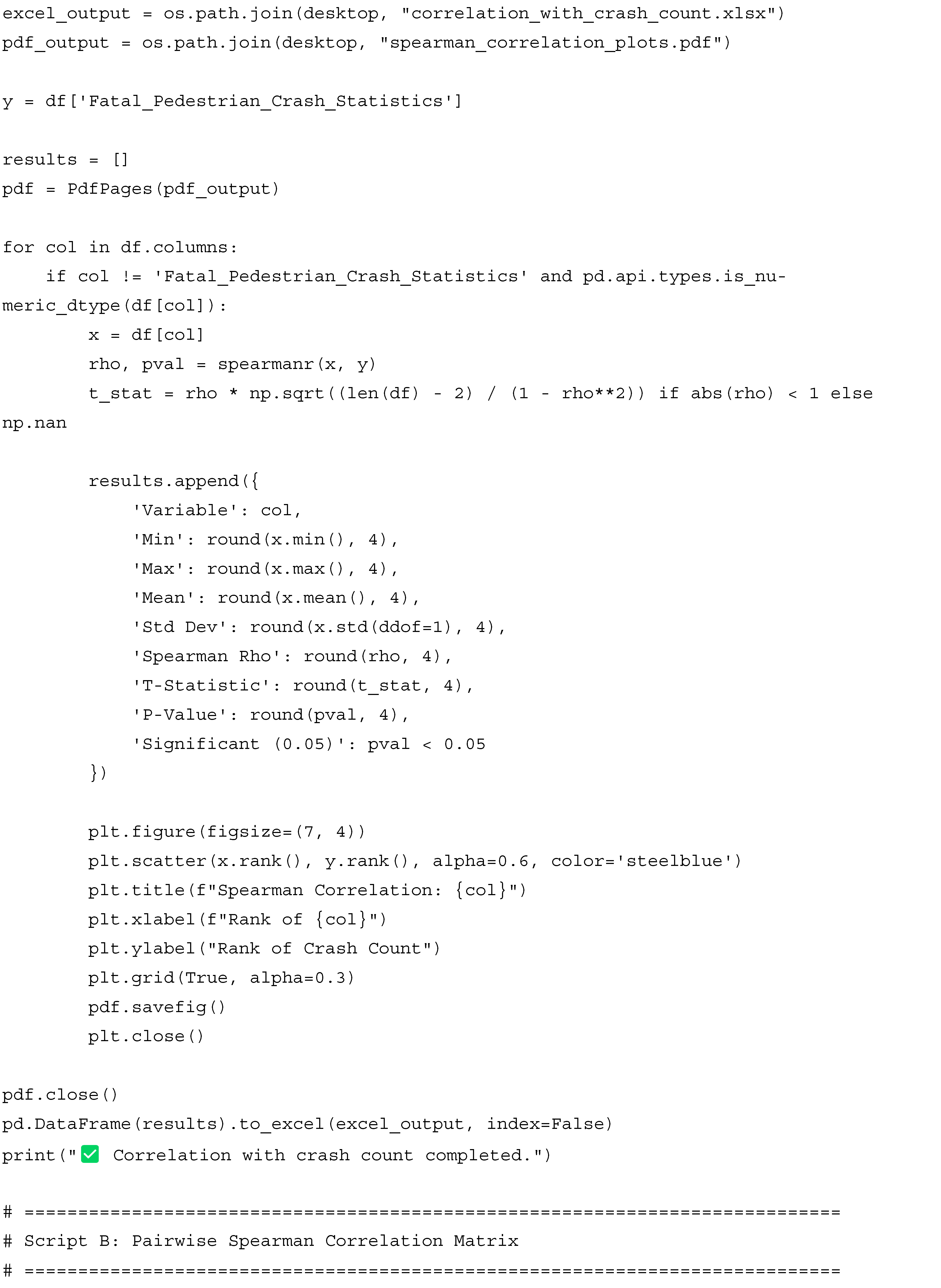
Appendix C. Python Scripts for Spearman’s Correlation, Negative Binomial Modelling with Model Fit Metrics



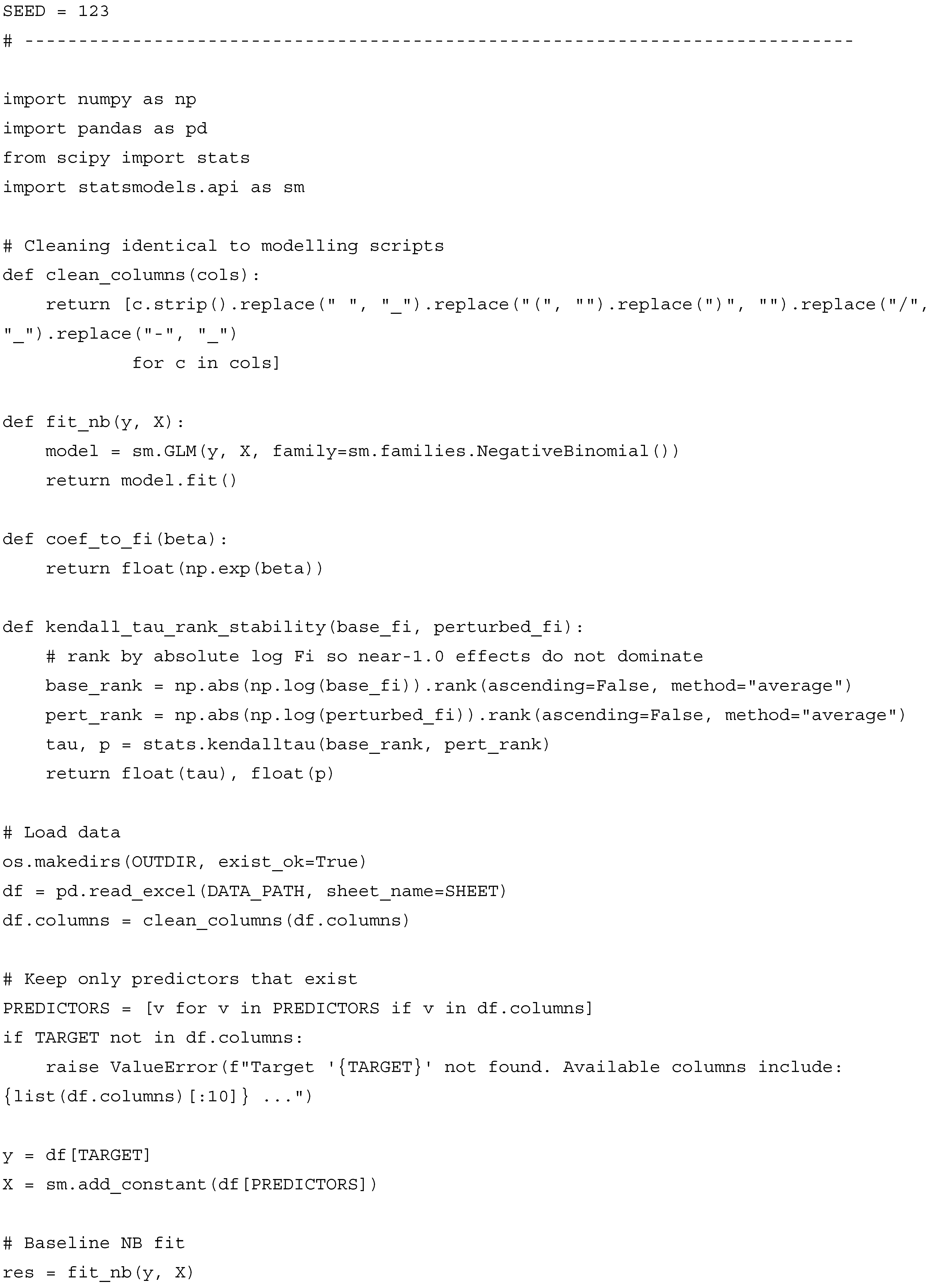
Appendix D. Python Code for Sensitivity Analysis and Fi Uncertainty Check




References
- WHO. Pedestrian Safety: A Road Safety Manual for Decision-Makers and Practitioners; World Health Organisation: Geneva, Switzerland, 2023. [Google Scholar]
- Karathodorou, N.; Graham, D.; Richter, T.; Ruhl, S.; La Torre, F.; Domenichini, L.; Yannis, G.; Dragomanovits, A.; Laio, A. Development of a crash modification factors model in Europe. In Proceedings of the 17th International Conference Road Safety On Five Continents (RS5C 2016), Rio de Janeiro, Brazil, 17–19 May 2016. Statens väg-och transportforskningsinstitut. [Google Scholar]
- National Academies of Sciences, Engineering, and Medicine. Pedestrian Safety Prediction Methodology; The National Academies Press: Washington, DC, USA, 2008. [Google Scholar]
- Kraidi, R.; Evdorides, H. Pedestrian safety models for urban environments with high roadside activities. Saf. Sci. 2020, 130, 104847. [Google Scholar] [CrossRef]
- Job, R.S.; Wambulwa, W.M. Features of low-income and middle-income countries making road safety more challenging. J. Road Saf. 2020, 31, 79–84. [Google Scholar] [CrossRef]
- Thierry, M.; Vet, J.; Uddin, K.B.; Wegman, F. A New Methodology for Road Crash Data Collection in Bangladesh Using Local Record Keepers. J. Road Saf. 2023, 34, 1–11. [Google Scholar] [CrossRef]
- Mubiru, J.; Evdorides, H. Pedestrian Safety in Developing Countries: A Systematic Literature Review & Gap Analysis; Manuscript under review in the Journal of Future Transportation; University of Birmingham: Birmingham, UK, 2025. [Google Scholar]
- Lin, P.-S.; Guo, R.; Bialkowska-Jelinska, E.; Kourtellis, A.; Zhang, Y. Development of countermeasures to effectively improve pedestrian safety in low-income areas. J. Traffic Transp. Eng. (Engl. Ed.) 2019, 6, 162–174. [Google Scholar] [CrossRef]
- Mukherjee, D.; Mitra, S. Identification of Pedestrian Risk Factors Using Negative Binomial Model. Transp. Dev. Econ. 2020, 6, 4. [Google Scholar] [CrossRef]
- Mukherjee, D.; Mitra, S. Modelling risk factors for fatal pedestrian crashes in Kolkata, India. Int. J. Inj. Control Saf. Promot. 2020, 27, 197–214. [Google Scholar] [CrossRef]
- Parker, C.; Scott, S.; Geddes, A. Snowball sampling. In SAGE Research Methods Foundations; 2019. Available online: https://eprints.glos.ac.uk/6781/1/6781%20Parker%20and%20Scott%20%282019%29%20Snowball%20Sampling_Peer%20reviewed%20pre-copy%20edited%20version.pdf (accessed on 16 June 2025).
- Caird, J.K.; Willness, C.R.; Steel, P.; Scialfa, C. A meta-analysis of the effects of cell phones on driver performance. Accid. Anal. Prev. 2008, 40, 1282–1293. [Google Scholar] [CrossRef]
- Sundaram, J.; Gowri, K.; Devaraju, S.; Gokuldev, S.; Jayaprakash, S.; Anandaram, H.; Manivasagan, C.; Thenmozhi, M. An Exploration of Python Libraries in Machine Learning Models for Data Science. In Advanced Interdisciplinary Applications of Machine Learning Python Libraries for Data Science; Biju, S.M., Mishra, A., Kumar, M., Eds.; IGI Global Scientific Publishing: Hershey, PA, USA, 2023; pp. 1–31. [Google Scholar]
- Harris, C.R.; Millman, K.J.; van der Walt, S.J.; Gommers, R.; Virtanen, P.; Cournapeau, D.; Wieser, E.; Taylor, J.; Berg, S.; Smith, N.J.; et al. Array programming with NumPy. Nature 2020, 585, 357–362. [Google Scholar] [CrossRef] [PubMed]
- Virtanen, P.; Gommers, R.; Oliphant, T.E.; Haberland, M.; Reddy, T.; Cournapeau, D.; Burovski, E.; Peterson, P.; Weckesser, W.; Bright, J.; et al. SciPy 1.0: Fundamental algorithms for scientific computing in Python. Nat. Methods 2020, 17, 261–272. [Google Scholar] [CrossRef] [PubMed]
- Freedman, D.A. Statistical Models: Theory and Practice; Cambridge University Press: Cambridge, UK, 2009. [Google Scholar]
- Lee, A. Generating random binary deviates having fixed marginal distributions and specified degrees of association. Am. Stat. 1993, 47, 209–215. [Google Scholar] [CrossRef]
- McKinney, W. Python for Data Analysis: Data Wrangling with Pandas, NumPy, and IPython; O’Reilly Media, Inc.: Sebastopol, CA, USA, 2012. [Google Scholar]
- Yim, A.; Chung, C.; Yu, A. Matplotlib for Python Developers: Effective Techniques for Data Visualization with Python; Packt Publishing Ltd.: Birmingham, UK, 2018. [Google Scholar]
- Altman, D.G.; Bland, J.M. Standard deviations and standard errors. BMJ 2005, 331, 903. [Google Scholar] [CrossRef]
- Rice, J.A.; Rice, J.A. Mathematical Statistics and Data Analysis; Thomson/Brooks/Cole Belmont: Monterey, CA, USA, 2007; Volume 371. [Google Scholar]
- Montgomery, D.C.; Runger, G.C. Applied Statistics and Probability for Engineers; John Wiley & Sons: Hoboken, NJ, USA, 2010. [Google Scholar]
- Hauke, J.; Kossowski, T. Comparison of values of Pearson’s and Spearman’s correlation coefficients on the same sets of data. Quaest. Geogr. 2011, 30, 87–93. [Google Scholar] [CrossRef]
- Mukherjee, D.; Mitra, S. Pedestrian safety analysis of urban intersections in Kolkata, India using a combined proactive and reactive approach. J. Transp. Saf. Secur. 2022, 14, 754–795. [Google Scholar] [CrossRef]
- Cameron, A.C.; Trivedi, P.K. Regression Analysis of Count Data; Cambridge University Press: Cambridge, UK, 2013. [Google Scholar]
- Washington, S.; Karlaftis, M.G.; Mannering, F.; Anastasopoulos, P. Statistical and Econometric Methods for Transportation Data Analysis; Chapman and Hall/CRC: Boca Raton, FL, USA, 2020. [Google Scholar]
- David Freeman, R.P.; Purves, R. Statistics, 4th ed.; W.W. Norton & Company: New York, NY, USA, 2007. [Google Scholar]
- iRAP. iRAP Specification, Manuals and Guides. 2021. Available online: https://irap.org/specifications/ (accessed on 31 July 2025).
- Earth.Org. Millions of Highly-Polluting Used Cars “Dumped” on Developing Countries-UN. 2020. Available online: https://earth.org/cars-developing-countries/ (accessed on 15 August 2025).
- Heydari, S.; Hickford, A.; McIlroy, R.; Turner, J.; Bachani, A.M. Road safety in low-income countries: State of knowledge and future directions. Sustainability 2019, 11, 6249. [Google Scholar] [CrossRef]
- Chowdhury, T.; Rifaat, S.M.; Tay, R. Characteristics of Pedestrians in Bangladesh Who Did Not Receive Public Education on Road Safety. Sustainability 2022, 14, 9909. [Google Scholar] [CrossRef]
- Shaaban, K. Impact of experience and training on traffic knowledge of young drivers. Open Transp. J. 2021, 15, 61–68. [Google Scholar] [CrossRef]
- Mukherjee, D.; Mitra, S. Comprehensive Study of Risk Factors for Fatal Pedestrian Crashes in Urban Setup in a Developing Country. Transp. Res. Rec. 2020, 2674, 100–118. [Google Scholar] [CrossRef]
- Victoria Transport Policy Institute. Developing Country Transport Demand Management: Transportation Demand Management in Lower-Income Regions. 2019. Available online: https://www.vtpi.org/tdm/tdm75.htm (accessed on 15 August 2025).
- Frimpong, L.K. Enhancing Pedestrian Safety in African Cities. 2022. Available online: https://www.researchgate.net/publication/363415723_Enhancing_Pedestrian_Safety_in_African_Cities#fullTextFileContent (accessed on 15 August 2025).
- Jia, W.; Tesfaye, B.; Alcala, Y.M. How Can We Make Cities Safer for Pedestrians? Some Insights from Ethiopia. 2022. Available online: https://blogs.worldbank.org/en/transport/how-can-we-make-cities-safer-pedestrians-some-insights-ethiopia (accessed on 15 August 2025).
- Walelign Bishaw, T.; Dolebo, G.N.; Singh, R.B. Evaluating pedestrian facilities for enhancing pedestrian safety in Addis Ababa city. Front. Sustain. Cities 2024, 6. [Google Scholar] [CrossRef]
- Damsere-Derry, J.; Ebel, B.E.; Mock, C.N.; Afukaar, F.; Donkor, P.; Kalowole, T.O. Evaluation of the effectiveness of traffic calming measures on vehicle speeds and pedestrian injury severity in Ghana. Traffic Inj. Prev. 2019, 20, 336–342. [Google Scholar] [CrossRef]
- Osuret, J.; Namatovu, S.; Biribawa, C.; Balugaba, B.E.; Zziwa, E.B.; Muni, K.; Ningwa, A.; Oporia, F.; Mutto, M.; Kyamanywa, P.; et al. State of pedestrian road safety in Uganda: A qualitative study of existing interventions. Afr. Health Sci. 2021, 21, 1498–1506. [Google Scholar] [CrossRef]
- Sabi Boun, S.; Janvier, R.; Marc, R.E.J.; Paul, P.; Senat, R.; Demes, J.A.E.; Burigusa, G.; Chaput, S.; Maurice, P.; Druetz, T. Environmental measures to improve pedestrian safety in low- and middle-income countries: A scoping review. Glob. Health Promot. 2024, 31, 44–55. [Google Scholar] [CrossRef]
- Times News Network. Pedestrian Life a No-Go in Bhopal as BMC Sidesteps Duties & Fails to Walk the Talk. 2025. Available online: https://timesofindia.indiatimes.com/city/bhopal/pedestrian-life-a-no-go-in-bhopal-as-bmc-sidesteps-duties-fails-to-walk-the-talk/articleshow/121241233.cms (accessed on 15 August 2025).
- Bliss, T.; Breen, J.M. Road Safety Management Capacity Reviews and Safe System Projects Guidelines (Updated Edition); World Bank Group: Washington, DC, USA,, 2013; Available online: https://documents.worldbank.org/en/publication/documents-reports/documentdetail/400301468337261166 (accessed on 15 August 2025).
- Zhu, M.; Zhao, S.; Coben, J.H.; Smith, G.S. Why more male pedestrians die in vehicle-pedestrian collisions than female pedestrians: A decompositional analysis. Inj. Prev. 2013, 19, 227–231. [Google Scholar] [CrossRef]
- International Labour Organization. Labor Force Participation Rate, Total (% of Total Population Ages 15+) (Modeled ILO Estimate). 2025. Available online: https://data.worldbank.org/indicator/SL.TLF.CACT.ZS (accessed on 15 August 2025).
- Arisoy, N. Measuring students’ preferences for urban furniture vandalism in Selçuk University Campus in Turkey: A case study. Arch. Agric. Environ. Sci. 2020, 5, 426–430. [Google Scholar] [CrossRef]
- Zegeer, C.; Srinivasan, R.; Lan, B.; Carter, D.; Smith, S.; Sundstrom, C.; Thirsk, N.J.; Zegeer, J.; Lyon, C.; Ferguson, E.; et al. Development of Crash Modification Factors for Uncontrolled Pedestrian Crossing Treatments; National Academies of Sciences, Engineering, and Medicine: Washington, DC, USA, 2017; 162p. [Google Scholar] [CrossRef]
- Silverman, B.W. Density Estimation for Statistics and Data Analysis; Routledge: Oxfordshire, UK, 1986. [Google Scholar]
- Zafri, N.M.; Khan, A. A spatial regression modeling framework for examining relationships between the built environment and pedestrian crash occurrences at macroscopic level: A study in a developing country context. Geogr. Sustain. 2022, 3, 312–324. [Google Scholar] [CrossRef]
- Huang, H.; Abdel-Aty, M. Multilevel data and Bayesian analysis in traffic safety. Accid. Anal. Prev. 2010, 42, 1556–1565. [Google Scholar] [CrossRef]
- Yang, J.; Gauli, N.; Shiwakoti, N.; Tay, R.; Deng, H.; Chen, J.; Nepal, B.; Li, J. Examining the Factors Influencing Pedestrian Behaviour and Safety: A Review with a Focus on Culturally and Linguistically Diverse Communities. Sustainability 2025, 17, 6007. [Google Scholar] [CrossRef]
- Ghasedi, M.; Sarfjoo, M.; Bargegol, I. Prediction and Analysis of the Severity and Number of Suburban Accidents Using Logit Model, Factor Analysis and Machine Learning: A case study in a developing country. SN Appl. Sci. 2021, 3, 13. [Google Scholar] [CrossRef]
- Mukherjee, D.; Mitra, S. A comprehensive study on factors influencing pedestrian signal violation behaviour: Experience from Kolkata City, India. Saf. Sci. 2020, 124, 104610. [Google Scholar] [CrossRef]
- Tiwari, G. Progress in pedestrian safety research. Int. J. Inj. Control Saf. Promot. 2020, 27, 35–43. [Google Scholar] [CrossRef] [PubMed]
- Hossain, S.; Maggi, E.; Vezzulli, A. Factors influencing the road accidents in low and middle-income countries: A systematic literature review. Int. J. Inj. Control Saf. Promot. 2024, 31, 294–322. [Google Scholar] [CrossRef] [PubMed]
- Mukherjee, D. Analyzing key determinants of pedestrian risky behaviors at urban signalized intersections: Insights from Kolkata City, India. Int. J. Inj. Control Saf. Promot. 2025, 32, 201–229. [Google Scholar] [CrossRef] [PubMed]

| Variable/Factor | NB Coefficient (β) | Risk Factor Influence (Fi) = eβ | Bootstrap 95% Confidence Interval for Fi | ||
|---|---|---|---|---|---|
| Lower Bound (2.5th Percentile) | Median (50th Percentile) | Upper Bound (97.5th Percentile) | |||
| Log (Avg Daily Traffic Volume) | −0.150 | 0.86 | 0.910 | 1.126 | 1.380 |
| Log (Avg Daily Pedestrian Volume) | 0.10 | 1.11 | 0.862 | 0.982 | 1.113 |
| Speed (km/h) | 0.00 | 1.00 | 0.994 | 1.000 | 1.005 |
| Pedestrian/Vehicle Volume Ratio | 0.00 | 1.00 | 0.951 | 0.991 | 1.032 |
| Vehicle Age/Technology (%) | 0.15 | 1.16 | 0.634 | 0.918 | 1.364 |
| Road Use (%) | 0.05 | 1.05 | 0.806 | 1.009 | 1.278 |
| Design Configuration (%) | 0.13 | 1.14 | 0.603 | 0.841 | 1.150 |
| Ad hoc implementation of countermeasures (%) | −0.46 | 0.63 | 0.767 | 1.231 | 1.957 |
| Footpath Encroachment (%) | 0.00 | 1.00 | 0.785 | 0.900 | 1.026 |
| Age < 18 (%) | 0.06 | 1.06 | 0.921 | 1.316 | 1.867 |
| Age 18–49 (%) | 0.14 | 1.15 | 0.798 | 1.100 | 1.478 |
| Age 50+ (%) | −0.08 | 0.92 | 0.594 | 1.150 | 2.178 |
| Male Pedestrians (%) | 0.11 | 1.12 | 0.708 | 0.960 | 1.297 |
| Female Pedestrians (%) | −0.15 | 0.86 | 0.521 | 0.833 | 1.383 |
| Employed Population (%) | 0.20 | 1.22 | 0.832 | 1.318 | 2.187 |
| Maintenance Practices (%) | −0.10 | 0.90 | 0.702 | 1.097 | 1.714 |
| Pedestrian Infrastructure Coverage (%) | 0.07 | 1.07 | 0.407 | 0.632 | 0.973 |
| Street Furniture Vandalism | −0.03 | 0.97 | 0.901 | 0.998 | 1.109 |
| Age of Countermeasure (years) | −0.01 | 0.99 | 0.994 | 1.010 | 1.027 |
| Appropriate Countermeasure Location (1/0) | 0.04 | 1.04 | 0.891 | 0.980 | 1.079 |
| Scenario (Sample Size n and Noise Level) | Kendall’s τ | p-Value |
|---|---|---|
| n = 1000, noise = 1.0 | 0.611 | 0.000 |
| n = 1000, noise = 0.05 | 0.632 | 0.000 |
| n = 1000, noise = 0.10 | 0.695 | 0.000 |
| n = 2000, noise = 1.0 | 0.358 | 0.028 |
| n = 2000, noise = 0.05 | 0.337 | 0.040 |
| n = 2000, noise = 0.10 | 0.211 | 0.209 |
| n = 5000, noise = 1.0 | 0.442 | 0.006 |
| n = 5000, noise = 0.05 | 0.516 | 0.001 |
| n = 5000, noise = 0.10 | 0.558 | 0.000 |
| Variable/Factor | Coefficient (β) | Risk Factor (Fi) = eβ | In NB Model | iRAP Covered | Practical Notes |
|---|---|---|---|---|---|
| Log (Avg Daily Traffic Volume) | −0.150 | 0.86 | included | included | iRAP uses traffic flow |
| Log (Avg Daily Pedestrian Volume) | 0.10 | 1.11 | included | included | Pedestrian exposure proxy |
| Speed (km/h) | 0.00 | 1.00 | included | included | iRAP core attribute |
| Pedestrian/Vehicle Volume Ratio | 0.00 | 1.00 | included | excluded | Traffic exposure factor |
| Vehicle Age/Technology (%) | 0.15 | 1.16 | included | excluded | The age of the vehicle fleet is crucial in DCs |
| Overtaking Tendency | N/A | N/A | excluded | excluded | Critical in DCs |
| Traffic Rule Enforcement | N/A | N/A | excluded | excluded | Institutional variable |
| Public Safety Awareness (%) | N/A | N/A | excluded | excluded | Critical in DCs |
| Driver Safety Awareness (%) | N/A | N/A | excluded | excluded | Critical in DCs |
| Time of Day Visibility | N/A | N/A | excluded | included | Lighting is a proxy |
| Road Use (%) | 0.05 | 1.05 | included | included | Functional classification included |
| Design Configuration (%) | 0.13 | 1.14 | included | included | Includes medians, crossings, etc. |
| Ad hoc implementation of countermeasures (%) | −0.46 | 0.63 | included | excluded | Planning sequence not captured |
| Footpath Encroachment (%) | 0.00 | 1.00 | included | excluded | Informal sector factor |
| Human Capacity of Agencies | N/A | N/A | excluded | excluded | Institutional capacity—not modelled |
| Age < 18 (%) | 0.06 | 1.06 | included | included | covered under the Star rating for schools |
| Age 18–49 (%) | 0.14 | 1.15 | included | excluded | High-activity demographic |
| Age 50+ (%) | −0.08 | 0.92 | included | excluded | Vulnerable group not addressed |
| Male Pedestrians (%) | 0.11 | 1.12 | included | excluded | Demographic dimension |
| Female Pedestrians (%) | −0.15 | 0.86 | included | excluded | Gender exposure gap |
| Employed Population (%) | 0.20 | 1.22 | included | excluded | Mobility-related risk |
| Maintenance Practices (%) | −0.10 | 0.90 | included | included | Maintenance quality implied in iRAP |
| Pedestrian Infrastructure Coverage (%) | 0.07 | 1.07 | included | included | iRAP footpath attribute |
| Street Furniture Vandalism | −0.03 | 0.97 | included | excluded | Social disorder indicator |
| Age of Countermeasure (years) | −0.01 | 0.99 | included | excluded | Asset age is important in DCs |
| Appropriate Countermeasure Location (1/0) | 0.04 | 1.04 | included | included | Part of iRAP’s star logic |
Disclaimer/Publisher’s Note: The statements, opinions and data contained in all publications are solely those of the individual author(s) and contributor(s) and not of MDPI and/or the editor(s). MDPI and/or the editor(s) disclaim responsibility for any injury to people or property resulting from any ideas, methods, instructions or products referred to in the content. |
© 2025 by the authors. Licensee MDPI, Basel, Switzerland. This article is an open access article distributed under the terms and conditions of the Creative Commons Attribution (CC BY) license (https://creativecommons.org/licenses/by/4.0/).
Share and Cite
Mubiru, J.; Evdorides, H. Quantifying the Risk Impact of Contextual Factors on Pedestrian Crash Outcomes in Data-Scarce Developing Country Settings. Future Transp. 2025, 5, 151. https://doi.org/10.3390/futuretransp5040151
Mubiru J, Evdorides H. Quantifying the Risk Impact of Contextual Factors on Pedestrian Crash Outcomes in Data-Scarce Developing Country Settings. Future Transportation. 2025; 5(4):151. https://doi.org/10.3390/futuretransp5040151
Chicago/Turabian StyleMubiru, Joel, and Harry Evdorides. 2025. "Quantifying the Risk Impact of Contextual Factors on Pedestrian Crash Outcomes in Data-Scarce Developing Country Settings" Future Transportation 5, no. 4: 151. https://doi.org/10.3390/futuretransp5040151
APA StyleMubiru, J., & Evdorides, H. (2025). Quantifying the Risk Impact of Contextual Factors on Pedestrian Crash Outcomes in Data-Scarce Developing Country Settings. Future Transportation, 5(4), 151. https://doi.org/10.3390/futuretransp5040151


