Article

Transportation Link Risk Analysis Through Stochastic Link Fundamental Flow Diagram

by
Orlando Giannattasio
1,* and
Antonino Vitetta
2
1
DICATECh Dipartimento di Ingegneria Civile, Ambientale, Edile, del Territorio e di Chimica, Politecnico di Bari, 70125 Bari, Italy
2
DIIES Dipartimento di Ingegneria dell’Informazione, delle Infrastrutture e dell’Energia Sostenibile, Università degli Studi Mediterranea di Reggio Calabria, 89122 Reggio Calabria, Italy
*
Author to whom correspondence should be addressed.
Future Transp. 2025, 5(4), 150; https://doi.org/10.3390/futuretransp5040150
Submission received: 23 August 2025 / Revised: 8 October 2025 / Accepted: 10 October 2025 / Published: 21 October 2025

Abstract

This paper proposes a method for assessing societal risk along a traffic link by integrating a stochastic formulation of the fundamental diagram. The approach accounts for uncertainty in vehicle speed due to user heterogeneity, vehicle characteristics, and environmental conditions. The risk index is decomposed into occurrence, vulnerability, and exposure components, with the occurrence probability modeled as a function of stochastic speed. The inverse gamma distribution is adopted to represent speed variability, enabling analytical tractability and control over dispersion. Numerical results show that urban and suburban environments exhibit distinct sensitivity to model parameters, particularly the gamma shape parameter η and the composite parameter c = β · v0 obtained by the product of the occurrence parameter β and the free speed flow v0. Graphical representations illustrate the impact of uncertainty on risk estimation. The proposed framework enhances existing deterministic methods by incorporating probabilistic elements, offering a foundation for future applications in traffic safety management and infrastructure design.

1. Introduction

Road safety analysis increasingly requires the integration of probabilistic models to account for uncertainty in traffic behavior. Traditional deterministic approaches often overlook the variability introduced by heterogeneous users, diverse vehicle types, and fluctuating environmental conditions. This paper addresses this gap by proposing a stochastic formulation of the fundamental diagram (S-FD) and applying it to the assessment of societal risk along a traffic link.
The societal risk index is decomposed into three components: occurrence, vulnerability, and exposure. This decomposition aligns with established risk assessment frameworks in transportation and other safety-critical domains as explained in [1,2,3,4].
The main research question addressed in this study is as follows: how does the societal risk index vary along a traffic link when speed is modeled as a random variable via an S-FD, and what are the implications for traffic safety assessment?
To answer this, we develop a mathematical method that integrates stochastic speed modeling with risk quantification. The inverse gamma (InvGamma) distribution is adopted to represent speed variability, offering analytical tractability and control over dispersion. The proposed method is applied to both urban and suburban traffic scenarios, highlighting differences in sensitivity to model parameters.
This paper is organized as follows. Section 2 introduces the S-FD and its properties. Section 3 presents risk formulation. Section 4 details the mathematical model. Section 5 provides numerical results and graphical interpretations. Section 6 concludes with implications and future research directions.

2. Deterministic and Stochastic Link Fundamental Diagram

The fundamental diagram (FD) (also called the link fundamental flow diagram, LFFD) describes how vehicles move along a stretch of highway through relations among vehicle density, flow, and speed. Under steady-state conditions the FD is the most used traffic model. It was first proposed in [5]. Recent reviews of models of Traffic Flow Theory include [6,7,8,9,10,11,12]. Segment-level studies [13] underscored the importance of spatiotemporal flow variability in crash-frequency modeling.
Two basic variables can be observed for each link of a highway: flow, depending on space, and density, depending on time. Speed can be averaged on space or time; the former depends on the time instant, the latter on space.
Under steady-state conditions the flow during a time interval does not depend on the space, and the density and the (space average) speed over a stretch of space do not depend on the instant of time. If
  • f ≥ 0 is the (vehicular) flow;
  • k ≥ 0 is the (vehicular) density;
  • v ≥ 0 is the (space average) speed;
  • fMAX is the capacity (f ≤ fMAX is commonly assumed as a function of geometrical characteristics of the infrastructure [7] or calibrated against read data);
  • kMAX is the maximum density (k ≤ kMAX, depending on (average) vehicle length and minimum safety distance or calibration against read data);
  • v0 is the zero-flow or free-flow or maximum speed (v ≤ v0 is commonly assumed as a function of geometrical characteristics of the infrastructure, as well as weather and light conditions),
the following relation holds:
f = k · v
Moreover, a relationship between density and speed holds, defined by the monotonically decreasing speed–density function:
v = vK(k) ∈ [0, v0]   0 ≤ k ≤ kMAX
Combining Equations (1) and (2) the flow–density function is defined as
f = f(k)∈ [0, fMAX]   0 ≤ k ≤ kMAX
with f(k) = k · vK(k); vice versa, knowing the f(k) function, the speed–density function is easily defined as vK(k) = f(k)/k.
Two further (endogenous–model-dependent) parameters can be defined:
  • kC is the critical density, the density giving the maximum flow f(kC) = fMAX;
  • vC = vK(kC) is the critical speed, the speed at critical density.
The flow–density function is monotonically increasing up to the critical density (stable regime), then decreases (unstable regime).
Finally, a relationship holds between speed and flow, obtained from Equations (1) and (2), when looking for the solutions of the equation v − vK(f/v) = 0:
v = v(f) ∈ [0, v0]   0 ≤ f ≤ fMAX
Two regimes, with two different values of speed, correspond to each value of flow:
  • A stable regime, with high speed and low density, in which v(f) is monotonically decreasing;
  • An unstable regime, with low speed and high density, in which v(f) is monotonically increasing.
When steady-state conditions do not hold, within-day dynamic macroscopic models can be used, including the FD or S-FD as one of the main equations.
The above deterministic analysis does not consider several sources of uncertainty such as users’, vehicles’, and infrastructures’ heterogeneity, weather and light conditions, etc. Therefore, it seems useful to carry out a stochastic analysis too, where the speed given by the stable regime speed–flow function is to be considered the mean of a random variable V, whose dispersion models some sources of uncertainty, leading to the S-FD [9,10]:
v ⇜ V ∈ [0, v0]
such that E[V|f] = v(f), and there is possibly variance depending on flow too. In this paper the S-FD is within the risk assessment methods for endogenous events inside the flow.
The most promising distribution for speed seems to be InvGamma, which leads to link travel time (or link disutility) being distributed in a gamma distribution (Section 4), and thus to the use of the Gammit route choice model [9,14].

3. Transportation Link Risk Analysis

The probabilistic decomposition of road-traffic risk into occurrence, vulnerability, and exposure can be dated back to May [15], who first formalized the need to quantify crash likelihood as a function of dynamic flow variables, and was further elaborated in [16] through statistical linkage of observable traffic conflicts to safety outcomes. The role of flow instability in triggering endogenous events was clarified in [17], whose three-phase theory showed how minor speed perturbations escalate into breakdowns and shockwaves, elevating the probability of rear-end and lane-change collisions. Vulnerability curves grounded in impact kinematics emerged in [18], demonstrating the nonlinear escalation of crash severity with relative speed, and were refined in [19] to account for vehicle mass and braking performance. Exposure estimation, linking traffic density and speed, relies on the fundamental diagram reviewed in the next section.
This section summarizes the findings of a quantitative analysis investigating the relationship between risk parameters and mean travel speed in a transport network link [20]. The analysis is carried out separately for each of the three risk components for social risk.
The risk analysis model considers the following three components (Figure 1).
  • Occurrence. In the context of a transport system, a dangerous occurrence refers to an event, either accidental or intentional, that has the potential to cause serious harm, injury, or damage, and is often subject to specific reporting requirements. The occurrence of dangerous events in a transport system can be classified into two categories with respect to the vehicular flow:
    o 
    Exogenous: these events originate from external sources and, as a result, are not affected by congestion; some examples of this kind of event are floods and earthquakes;
    o 
    Endogenous: these events are generated by vehicle flow and congestion and thus depend on traffic conditions; examples of such events include vehicular accidents.
  • Vulnerability. In a transport system, vulnerability to dangerous events refers to the susceptibility of the system to disruptions and negative impacts caused by unforeseen or hazardous occurrences. The impact energy applied to users in the aftermath of a dangerous event can be quantified as follows:
    o 
    For an exogenous event occurring within the flow, the energy does not depend on the traffic flow variables;
    o 
    For endogenous events, the energy depends on the traffic flow variables and is mainly a function of the kinetic energy of the vehicles involved in the impact.
  • Exposure. In a transport system, exposure to dangerous events refers to the number of users (and the quantity of goods) on the link and in the proximity of the link who are affected by the hazardous event. The model is composed of two components:
    o 
    The first category of users is those situated close to the link, for example, residents, who could potentially be affected by the dangerous event;
    o 
    The second category of users is those utilizing the transport link; this category of users is dependent on traffic conditions.
Let
  • v be the (space average) speed;
  • pO be the probability of the occurrence of a hazardous event;
  • pO,EX be the probability of the occurrence of an exogenous hazardous event;
  • pO,EN1 be the probability of the occurrence of an endogenous dangerous event in an unstable flow region;
  • pO,EN2 be the probability of the occurrence of an endogenous dangerous event in a stable flow region;
  • pV be the vulnerability, the conditional probability that the users of the transport system will suffer negative effects given the occurrence of the dangerous event;
  • pV,EX be the vulnerability, the conditional probability given the occurrence of the dangerous exogenous event;
  • pV,EN be the vulnerability, the conditional probability given the occurrence of the dangerous endogenous event;
  • e be the exposure, the number of people (and the quantity of goods) exposed to exogenous (eEX) and endogenous (eEN) events.
The risk r, which is the mean number of people suffering negative effects, can be given by the following (see Figure 1):
r = pO · pV · e = pO,EX · pV,EX · (eEX + eEN) + (pO,EN1 + pO,EN2) · pV,EN · eEN
This paper describes the application of the proposed model to the risk of endogenous events only (assuming pO,EX, pV,EX, and eEX are equal to 0); under these assumptions, the Equation (6) becomes
r = pO · pV · e = (pO,EN1 + pO,EN2) · pV,EN · eEN
In the case of only a stable flow region (pO,EN1 is equal to 0), the risk is
r = pO,EN2 · pV,EN · eEN

4. Transportation Link Risk Analysis Through Stochastic Fundamental Diagram

In a link, as indicated in Equation (8), societal risk is determined by three key components: occurrence, vulnerability, and exposure. In the specific case of a stable flow regime, these components can be expressed as functions of speed, which serves as the primary independent variable (within the assignment model framework):
pO,EN2 = pO,EN2(v)
pV,EN = pV,EN(v)
eEN = eEN(v)
Considering the stable regime of the traffic flow diagram, the travel speed v, or the travel time t (reciprocal of speed with length as the proportionality parameter), is a function of the flow f (or the density), v = v(f), described in Section 2. Therefore, societal risk can be specified as dependent on flow as well as some parameters (to keep the notation simple, the parameters were omitted from the risk function):
r(v(f), f) = pO,EN2(v(f)) · pV,EN(v(f)) · eEN(v(f))
According to the S-FD the speed–flow function provides the mean of the speed assumed as a random variable described by the probability density function (pdf). Two approaches (deterministic or stochastic) may be followed to compute the above risk index, as described below.

4.1. Deterministic Approach

If the randomness of the speed is neglected, each of the three components of societal risk provides a deterministic value and therefore the risk is deterministically defined.
Let
  • x = f/fMAX be the (dimensionless) degree of saturation;
  • y = v/v0 be the (dimensionless) speed ratio.
In most speed functions speed v depends on the degree of saturation x only; moreover, the speed can be expressed as the free flow speed (or maximum speed) times the speed ratio y, a function of the degree of saturation x:
y = y(x) ∈ [0,1]
Thus Equation (4) becomes:
v(f) = y(x) · v0 ∈ [0, v0]
Then, combining Equations (12) and (14), the risk (12) can be computed as a function of the degree of saturation, only as
r(v(f), f) = r(y(x) · v0, x · fMAX)

4.2. Stochastic Approach

If the speed is modeled as a random variable, each of the three components of societal risk is a function of a random variable; therefore, societal risk is defined by a random variable. According to the S-FD the speed–flow function provides the mean of the speed assumed as a continuous random variable, with the following sensible requirements:
  • Defined over the nonnegative real line;
  • Defined by at least scale and shape parameters, so that mean and variance are independent;
  • Unimodal;
  • Has an easily defined unimodal inverse describing the travel time randomness, stable with respect to the sum, thus allowing the modeling of route travel time as a random variable of known distribution.
Let v denote the space-averaged speed of vehicles on the link. In the S-FD, v is modeled as a random variable VInvGamma(η, θ), where
  • η is the shape parameter;
  • θV is the scale parameter.
The InvGamma distribution is defined by the probability density function:
fV(v) = θ . (Vη/Γ(η)) . vη−1 . eθv/v, v > 0
This choice also ensures nonnegativity, unimodality, and flexibility in controlling dispersion. In practical terms, lower values of η correspond to higher uncertainty in speed, which may reflect poorly controlled traffic environments or high heterogeneity among users and vehicles. Higher values of η indicate more stable speed distributions, typical of well-regulated traffic conditions.
The deterministic FD is recovered as a special case when η→∞, leading to a degenerate distribution where speed becomes constant.
The most promising distribution for the speed ratio Y according to the above requirements seems to be the one where the InvGamma that leads to travel time T is distributed as a gamma with scale parameters θT and the same shape parameter η; thus, μT = θT · η, and variance σT2 = θT2 · η.
The travel time gamma r. v. T may also be parameterized with respect to the mean μT and the shape parameter η; thus, the scale parameter is θT = μT/η and the variance is σT2 = μT2/η.
Assuming that the mean of T is given by the travel time function, μT = t(f), the travel time gamma r. v. T has shape parameter η, scale parameter θT = t(f)/η, and variance σT2 = t(f)2. Therefore T/t0 is a gamma r. v. with the same shape parameter η, mean μT/t0 = t(f)/t0, scale parameter θT/t0 = t(f)/(η · t0), and variance σT/t02 = t(f)2/(t02 · η).
Then the speed ratio r. v. Y = 1/(T/t0) is distributed as an InvGamma with the same shape parameter η, mean μY = (t0/t(f)) · (η /(η − 1)), scale parameter θY = (t0/t(f)) · η, and variance σY2 = (t0/t(f))2 · η2/((η − 1)2 · (η − 2)). Since t0/ t(x · fMAX) = y(x),
μY(x) = y(x) · η/(η − 1)
σY(x) = y(x) · η/((η − 1) · √(η − 2)) = μY(x)/√(η − 2)
In the stable regime, with η fixed, an increase in the degree of saturation x leads to a decrease in the speed ratio y(x), along with a reduction in the standard deviation. Within the same stable regime, for a given y(x), the standard deviation also decreases as η increases.
Thus, the coefficient of variants Y is
cv = σY(x, η)/μY(x) = 1/√(η − 2)
Independent of the degree of saturation, it decreases as η increases.
To guarantee positiveness of the mean, μY > 0, the shape parameter must be greater than 1; for that of the standard deviation, σY > 0, the shape parameter must be greater than 2; moreover, to avoid the coefficient of variation being greater than 1, the shape parameter must be greater than 3. Therefore, in the following the shape parameter is assumed to be greater than or equal to 3, η ≥ 3. It is worth noting that σY = μY for η = 3.
The explicit definition of the closed form of the pdf of the risk given the pdf of speed may be very cumbersome, as in most such cases Monte Carlo techniques could be applied, as will be addressed in a future paper. Otherwise, a heuristic approach (referred to as the H-Method) can be applied, as described below.
H-Method: Given v0 and fMAX, for each value of the degree of saturation x, a heuristic approach to the stochastic analysis of the risk is based on defining an interval for the risk index specified in Equation (15) by computing it for three values of speed ratio y(x):
yR(x) = μY(x) + σY(x)
yM(x) = μY(x)
yL(x) = μY(x) − σY(x)
For values of the shape parameter greater than or equal to 3, η ≥ 3, Equation (20c) always gives a nonnegative value. Equation (20a) may give values greater than 1 for low values of the shape parameter, or even greater than 3.
A more precise approach based on the definition of the risk index distribution from Equation (12) and the distribution of the speed will be discussed in a future paper. Since a closed-form formulation seems hard to derive, presumably Monte Carlo techniques need to be applied.
As a reminder for the reader, we provide a short glossary in Table 1 for faster reading.

5. Numerical Experimentation

The procedure is tested on a single link to check its applicability. The risk and traffic flow functions are specified, and risk curves are calculated using both deterministic and stochastic risk approaches.

5.1. Speed–Flow Function Specification

The FD can be derived from the well-known BPR-like travel time function, often used for transportation supply analysis and demand assignment:
t(f) = t0 · (1 + a (f /fMAX)b) 0 ≤ f ≤ fMAX
where
  • t is the travel time needed to traverse the link;
  • L is the length of the link;
  • t0 = L/v0 is the null flow travel time needed to traverse the link;
  • a > 1 is the congestion factor, such that 1 + a = t(fMAX)/t0;
  • b ≥ 1 is a shape coefficient (b = 1, meaning it is a linear function).
The stable regime speed–flow function, v(f) = L/t(f), corresponding to the BPR-like time–flow Equation (21) is given by
v(f) = v0/(1 + a (f/fMAX)b) 0 ≤ f ≤fMAX
Commonly used values of parameters are as follows (alternative parameter values may be adopted depending on the characteristics of the infrastructure and the flow, and should be calibrated using empirical data):
  • a = 0.15, b = 4, v0 = 120 km/h for extra-urban application [in this case Equation (21) mainly plays the role of a capacity constraint];
  • a = 2, b = 2, v0 = 60 km/h for urban application.
The speed–flow Equation (22) can be redefined as
y(x; a, b)= 1/(1 + a(x)b)∈ [0,1] 0 ≤ x ≤ 1
where
  • x = f/fMAX is the degree of saturation;
  • y = v/v0 is the speed ratio.

5.2. Risk Function Specification

The three components of the risk (occurrence, vulnerability, and exposure) in the following are specified as shown below [20]:
p0,EN2 = α1 · (1 − exp(−β · v))
pv,EN = α2 · (v/v0)2
eEN = α3 · L · k
where α1, α2, α3, and β are parameters greater than zero (to be calibrated against real data).
The above three equations can be combined with the speed flow Equation (2) in a stable flow region, such as (22); moreover, the density can be obtained from Equation (21) as k = f/v; thus,
p0,EN2(f) = α1 · (1 − exp(−β · v(f)))
pv,EN(f) = α2 · (v(f)/v0)2
eEN(f) = α3 · L · f /v(f)
Assuming α = α1 · α2 · α3, the risk–flow function (Equation (12)) for endogenous events is given by
r(f) = α · (1 − exp(−β · v(f))) (v(f)/v0)2 · L · f/v(f) =
= (α · L/v02) · (1 − exp(−β · v(f))) · v(f) · f =
= (α · L · fMAX/v0) (1 − exp(−β · v0 · v(f)/v0)) · (v(f)/v0) · (f/fMAX)
To enhance the clarity of exposition, the risk function and the speed function may include the model parameters, thereby making the dependence explicit:
r(f; a, b, c) = (α · L · fMAX/v0) (1 − exp(−c · v(f; a, b)/v0)) · (v(f; a, b)/v0) · (f/fMAX)
where c = β · v0 (β to be calibrated against real data).
A dimensionless risk index z in the range [0, 1] can be defined as
z(f; a, b, c) = r(f; a, b, c) · (v0/(α · L · fMAX))
The (dimensionless) risk index z(f; a, b, c) can be defined as a function of the degree of saturation, given by the multiplication of three terms, all in the range [0, 1]:
z(x; a, b, c) = (1 − exp(−c · y(x; a, b))) · y(x; a, b) · x ∈ [0, 1] 0 ≤ x ≤ 1
where (as already stated)
  • x = f/fMAX ∈ [0,1] is the degree of saturation (usually a value of fMAX = 2000 veic/h for a standard lane);
  • y = v/v0 ∈ [0, 1] is the speed ratio (usually values of v0 = 80–120 km/h x-urb, 30–60 km/h urb);
  • z = r/(α · L/v0 · fMAX) ∈ [0,1] is the risk index (L is the highway length; α is to be calibrated).

5.3. Numerical Results and Comments

This section presents the results of a deterministic or stochastic analysis using the formulation present in the previous section, namely Equations (23) and (31).
We apply the proposed risk model to two traffic environments: urban and suburban. The parameters a, b, and v0 are calibrated based on typical flow–speed profiles for each setting. Table 2 summarizes the input parameter values used, distinguishing urban and extra-urban settings, relative to the functions specified in Equations (22)–(24).
Despite using the same nominal capacity fmax = 2000 veic/h for both cases (which is the capacity known in the literature), the resulting risk profiles differ due to variations in the shape of the flow–speed function.

5.3.1. Deterministic Risk Analysis

Two types of deterministic analysis were carried out, concerning the speed ratio or risk index.
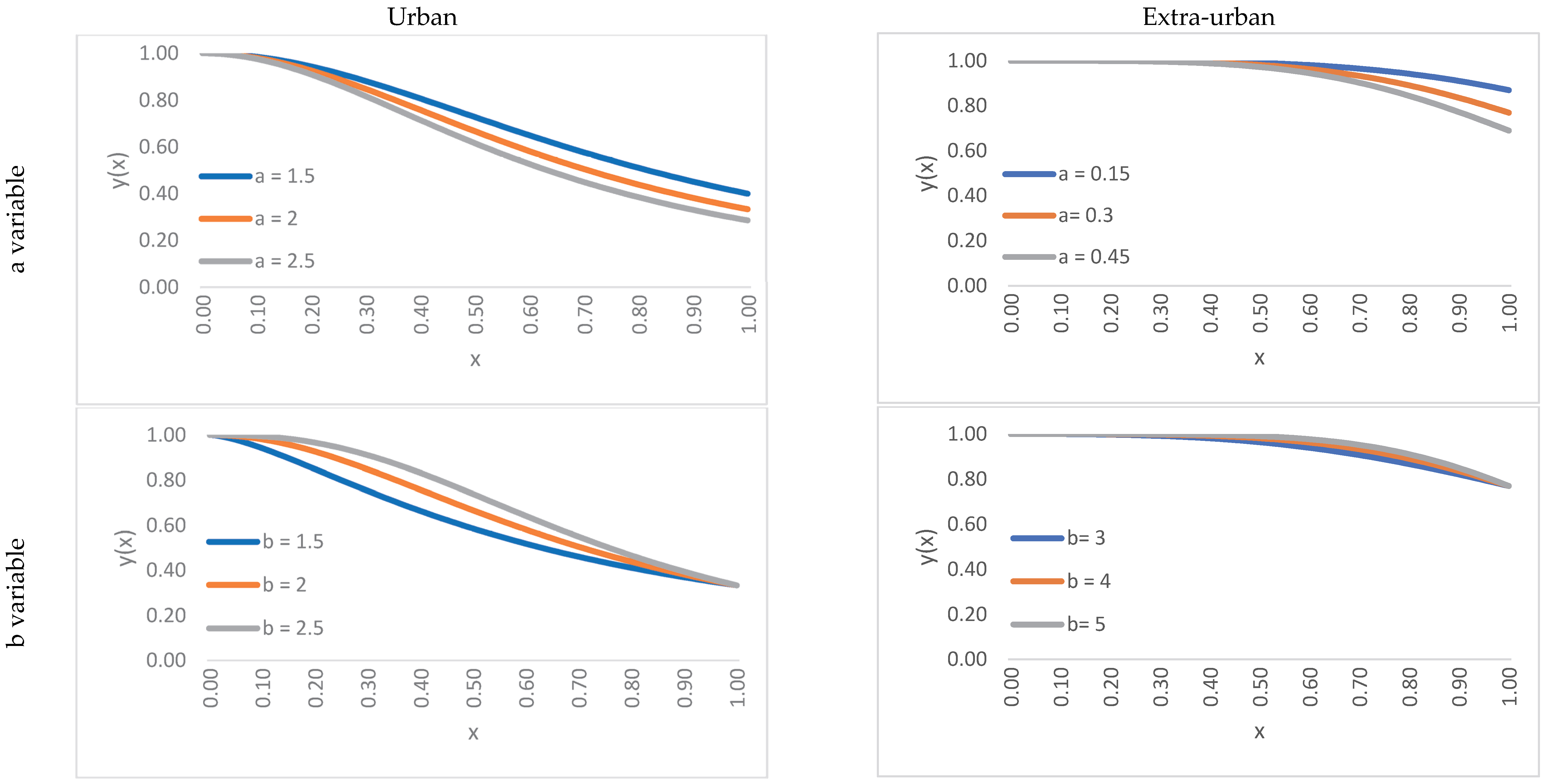
The first analysis compares the speed ratio values y() against the degree of saturation x considering different values of a and then of b in both urban and extra-urban settings (as shown in Figure 2). It is important to remember that since y() is not a function of c, it is useless to study the effect of changing such a parameter.
As far as the speed ratio y() is concerned, the effects of changing both parameters a and b are relevant in the urban setting, whilst for the extra-urban setting only changing parameter a has a significant effect. In both settings, as the degree of saturation goes to 0, the effect of changing parameter a becomes negligible, whilst as the degree of saturation goes to 0 or to 1 the effect of changing parameter b becomes negligible.
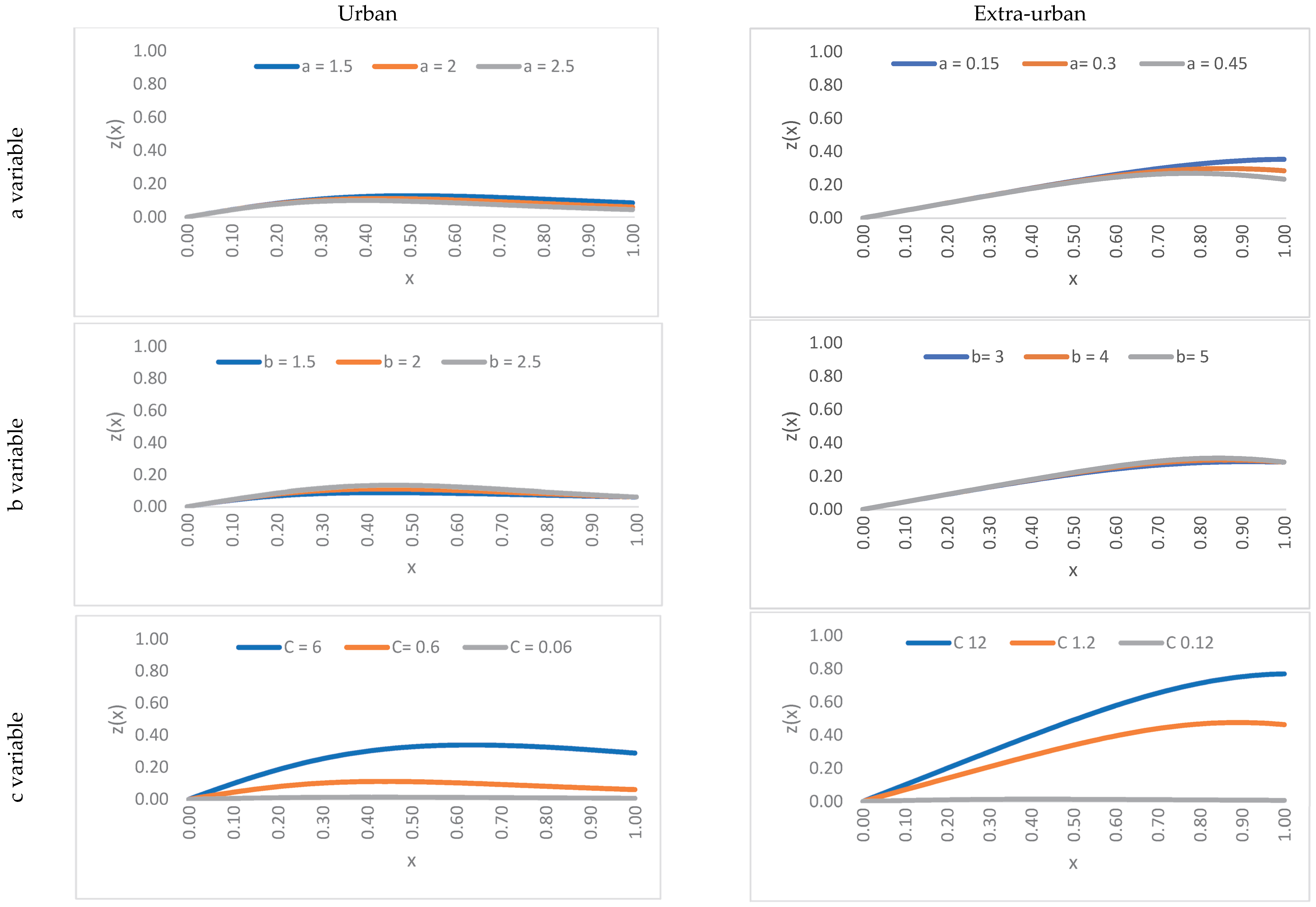
The second analysis compares the risk index values z() against the degree of saturation x in urban and extra-urban settings considering different values of a, b, and c (as shown in Figure 3); in any case z() against x shows a concave graph. Whatever the setting changes, both the parameters a and b have negligible effects. On the other hand, the effect of changing parameter c is very significant.
Figure 2 shows the impact of parameters a and b on the flow–speed relationship. In urban environments, both parameters significantly affect the curve, reflecting congestion sensitivity and speed deterioration. In suburban settings, parameter a dominates, consistent with highway flow characteristics.
Figure 3 illustrates the sensitivity of the risk index z(x) to the composite parameter c = βv0. We observe that higher values of c lead to sharper decay in occurrence probability and lower expected risk.

5.3.2. Stochastic Risk Analysis

Two types of stochastic analysis were carried out, concerning speed ratio or risk index, applying the H-Method defined above. The parameters used in this analysis are the same as those used for the deterministic analysis.
In both cases, as already stated, the speed ratio y is assumed to be a realization of the r.v. Y distributed as an InvGamma r.v. with mean μY given by y(), depending on the degree of saturation, and shape parameter η independent of the degree of saturation; from these two parameters, the standard deviation σY = μY/√(η − 2) can be obtained.
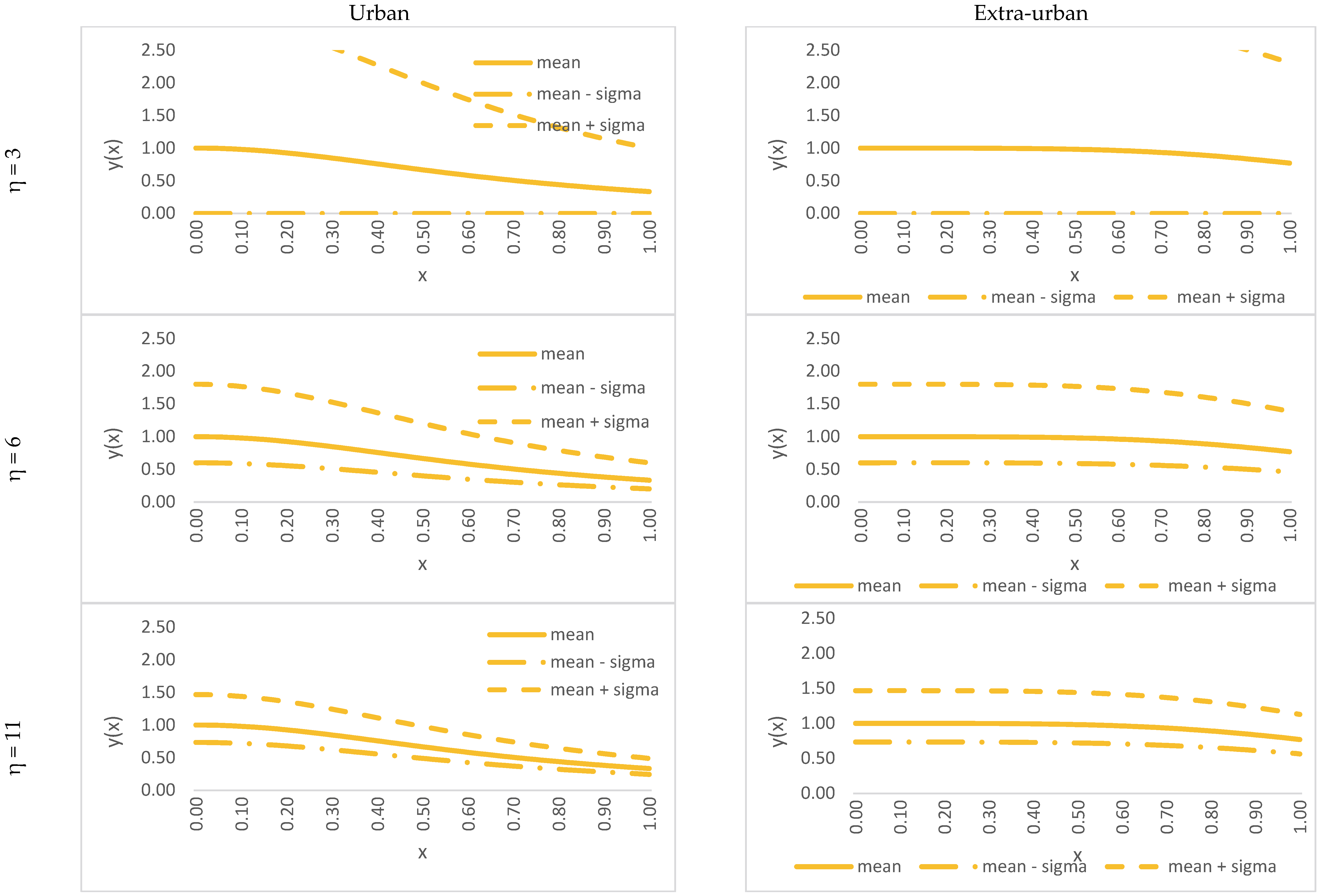
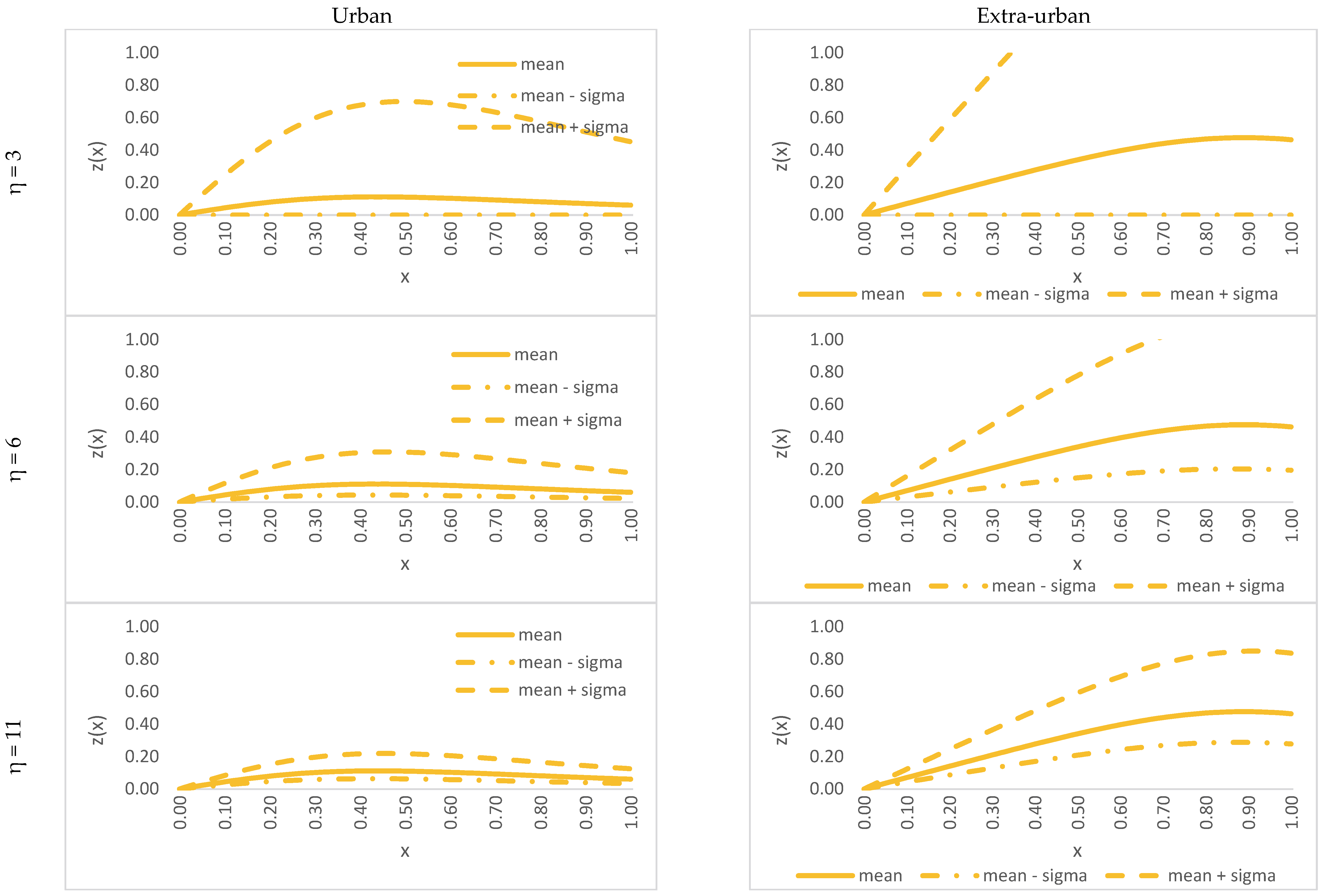
Figure 4 and Figure 5 show an uncertainty interval for the speed ratio y() or the risk index z(), respectively, against the degree of saturation x; the uncertainty interval is obtained by applying the H-Method, specified in Section 4.2, considering y as defined by Equations (20a), (20b) and (20c) respectively. Three values of shape parameter η are considered, 3, 6, and 11, corresponding to cv = 1, 1/2, and 1/3, according to Equation (19).
As expected, the larger the values of the shape parameter, the smaller the uncertainty interval. Figure 5 shows that the risk index is more sensitive to the degree of saturation and that uncertainty intervals are larger for the extra-urban setting with respect to urban ones. Lower η values yield wider intervals, indicating greater uncertainty in risk estimation. This has practical implications for traffic management: conservative measures may be warranted when uncertainty is high.
Some scenarios show a large uncertainty interval of the risk index for the extra-urban setting. These results, which are to be further investigated, may greatly affect the risk assessment for traffic control and project evaluation. Therefore, the Stochastic Risk Analysis results show how stochastic analysis allows us to obtain more effective results and can lead to interesting future developments to be discussed in future papers.
To quantify this effect, the elasticity index is adopted:
εc = ∂z/∂cc/z
Table 3 reports elasticity values for selected points along the link. The results confirm that z(x) is highly sensitive to c, especially in mid-range saturation levels.

6. Conclusions

A methodology has been proposed for the stochastic analysis of societal risk along a transportation link. This methodology further elaborates the approach to transportation risk analysis due to endogenous flow events proposed in [20]. Indeed, it includes a stochastic formulation of the (stable regime) fundamental flow diagram to consider the observed dispersion of the speed for each value of flow through a random variable.
Some specifications of the methodology have been discussed, and a heuristic implementation method has been formulated through dimensionless variables that are useful for providing uncertainty intervals for the speed as well as the risk index.
A heuristic method has been tested on a single link to check its applicability through some numerical applications to urban as well as extra-urban settings. Some scenarios show a large uncertainty interval of the risk index for the extra-urban setting; these results, to be further investigated, may greatly affect the risk assessment for traffic control and project evaluation.
Some issues worth further research efforts are as follows:
  • the combination of the proposed method with route choice models and its application within an assignment framework (recent reviews on this topic, introduced by Wardrop in his seminal paper [21], are in [22,23]);
  • the specification of a more precise modeling approach based on the definition of the risk index distribution from Equation (12) and the distribution of the speed as an InvGamma. Since a closed-form formulation seems hard to derive, presumably Monte Carlo techniques need to be applied.
This paper presents a stochastic framework for assessing societal risk along a traffic link, integrating uncertainty in vehicle speed via the InvGamma distribution. The proposed method extends traditional deterministic models by incorporating probabilistic elements, enabling more realistic and flexible risk estimation.
Numerical results demonstrate that urban and suburban environments respond differently to model parameters, particularly the shape parameter η and the composite parameter c = β · v0. Elasticity analysis confirms that the risk index is highly sensitive to these parameters, especially under medium saturation conditions.
The uncertainty interval associated with different values of η provides practical guidance for traffic safety management. Lower η values suggest greater variability in speed and risk, warranting conservative interventions. Higher η values indicate more stable conditions, allowing for targeted control strategies.
Future research will focus on implementing Monte Carlo simulations to refine the stochastic analysis and validate the model against empirical data. This will enhance the applicability of the framework in real-world traffic safety assessments and infrastructure planning.

Author Contributions

Data Curation, O.G.; Formal Analysis, O.G.; Methodology, A.V.; Supervision, A.V.; Validation, O.G.; Visualization, O.G.; Writing—original draft, A.V. and O.G.; Writing—review & editing, A.V. and O.G. All authors have read and agreed to the published version of the manuscript.

Funding

This research was partially supported by DIIES, Università degli Studi Mediterranea di Reggio Calabria, as part of the institutional support for co-author A.V.; this research was partially supported by DICATECh, Politecnico di Bari, as part of the institutional support for co-author O.G.

Data Availability Statement

All data used are reported in the paper.

Conflicts of Interest

The authors declare no conflict of interest.

References

  1. Ma, Y.; Xu, J.; Gao, C.; Mu, M.; E, G.; Gu, C. Review of Research on Road Traffic Operation Risk Prevention and Control. Int. J. Environ. Res. Public Health 2022, 19, 12115. [Google Scholar] [CrossRef] [PubMed]
  2. Zhao, C.; Chang, X.; Xie, T.; Fujita, H.; Wu, J. Unsupervised anomaly detection based method of risk evaluation for road traffic accident. Appl. Intell. 2023, 53, 369–384. [Google Scholar] [CrossRef]
  3. Berdica, K. An introduction to road vulnerability: What has been done, is done and should be done. Transp. Policy 2002, 9, 117–127. [Google Scholar] [CrossRef]
  4. Elvik, R. Some implications of an event-based definition of exposure to the risk of road accident. Accid. Anal. Prev. 2015, 76, 15–24. [Google Scholar] [CrossRef] [PubMed]
  5. Greenshields, B.D. A Study of Traffic Capacity. Highw. Res. Board Proc. 1935, 14, 448–477. [Google Scholar]
  6. Treiber, M.; Kesting, A. Traffic Flow Dynamics. In Traffic Flow Dynamics: Data, Models and Simulation; Springer: Berlin/Heidelberg, Germany, 2013. [Google Scholar]
  7. HCM. Highway Capacity Manual VI Edition, Transportation Research Board (TRB); National Academy of Sciences: Washington, DC, USA, 2016. [Google Scholar]
  8. Cantarella, G.E.; Watling, D.; De Luca, S.; Di Pace, R. Traffic Flow Theory. In Dynamics and Stochasticity in Transportation Systems; Elsevier: Amsterdam, The Netherlands, 2019. [Google Scholar]
  9. Cantarella, G.E.; Cipriani, E.; Gemma, A.; Giannattasio, O.; Mannini, L. Stochastic Fundamental Diagram Consistent with Transportation Systems Theory. In Proceedings of the 4th Symposium on Management of Future Motorway and Urban Traffic Systems 2022 (MFTS2022), Dresden, Germany, 30 November–2 December 2022. [Google Scholar]
  10. Cantarella, G.E.; Cipriani, E.; Gemma, A.; Giannattasio, O.; Mannini, L. Stochastic Fundamental Diagram: For motorway traffic modelling and emission estimation. Transp. Res. Procedia 2023, 12–18. [Google Scholar]
  11. Di Pace, R.; Cantarella, G.E. (Eds.) Urban Traffic Analysis and Control: The Key Challenges in the Era of ITS; IET: Stevenage, UK, 2025. [Google Scholar]
  12. Cascetta, E. Transportation Systems Analysis: Models and Applications; Springer Science & Business Media: Berlin/Heidelberg, Germany, 2009; Volume 29. [Google Scholar]
  13. Quddus, M.A.; Wang, C.; Ison, S.G. Road traffic congestion and crash severity: Econometric analysis using ordered response models. J. Transp. Eng. 2010, 136, 424–435. [Google Scholar] [CrossRef]
  14. De Luca, S. Choice Modelling Theories. Appendix 1 in Cantarella et al. In Dynamics and Stochasticity in Transportation Systems: Tools for Transportation Network Modelling; Elsevier: Amsterdam, The Netherlands, 2019. [Google Scholar] [CrossRef]
  15. May, A.D. Traffic Flow Fundamentals; Prentice Hall: Hoboken, NJ, USA, 1990. [Google Scholar]
  16. Hauer, E. Safety review of highway 407: Confronting two myths. Transp. Res. Rec. 1999, 1693, 9–12. [Google Scholar] [CrossRef]
  17. Kerner, B.S. The Physics of Traffic: Empirical Freeway Pattern Features, Engineering Applications, and Theory; Springer: Berlin/Heidelberg, Germany, 2004. [Google Scholar]
  18. Wier, M.; Weintraub, J.; Humphreys, E.H.; Seto, E.; Bhatia, R. An Area-Level Model of Vehicle-Pedestrian Collisions with Implications for Land Use and Transportation Planning. Accid. Anal. Prev. 2009, 41, 137–145. [Google Scholar] [CrossRef] [PubMed]
  19. Tarawneh, M.A.; Muromachi, Y. Vulnerability assessment by speed profiles. J. Traffic Transp. Eng. 2011, 11, 123–131. [Google Scholar]
  20. Vitetta, A. Influence of vehicular flow instability in a transport network on risk reduction: Test in a two-link network. J. Adv. Transp. 2025, 2025, 7966144. [Google Scholar] [CrossRef]
  21. Wardrop, J.G. Some Theoretical Aspects of Road Traffic Research. Proc. Inst. Civ. Eng. 1952, 2, 325–378. [Google Scholar] [CrossRef]
  22. Cantarella, G.E.; Watling, D.P.; de Luca, S.; Di Pace, R. Dynamics and Stochasticity in Transportation Systems: Tools for Transportation Network Modelling; Elsevier: Amsterdam, The Netherlands, 2019. [Google Scholar]
  23. Cantarella, G.E.; Fiori, C.; Mussone, L. Dynamics and Stochasticity in Transportation Systems: Equations and Examples; Elsevier: Amsterdam, The Netherlands, 2024. [Google Scholar]
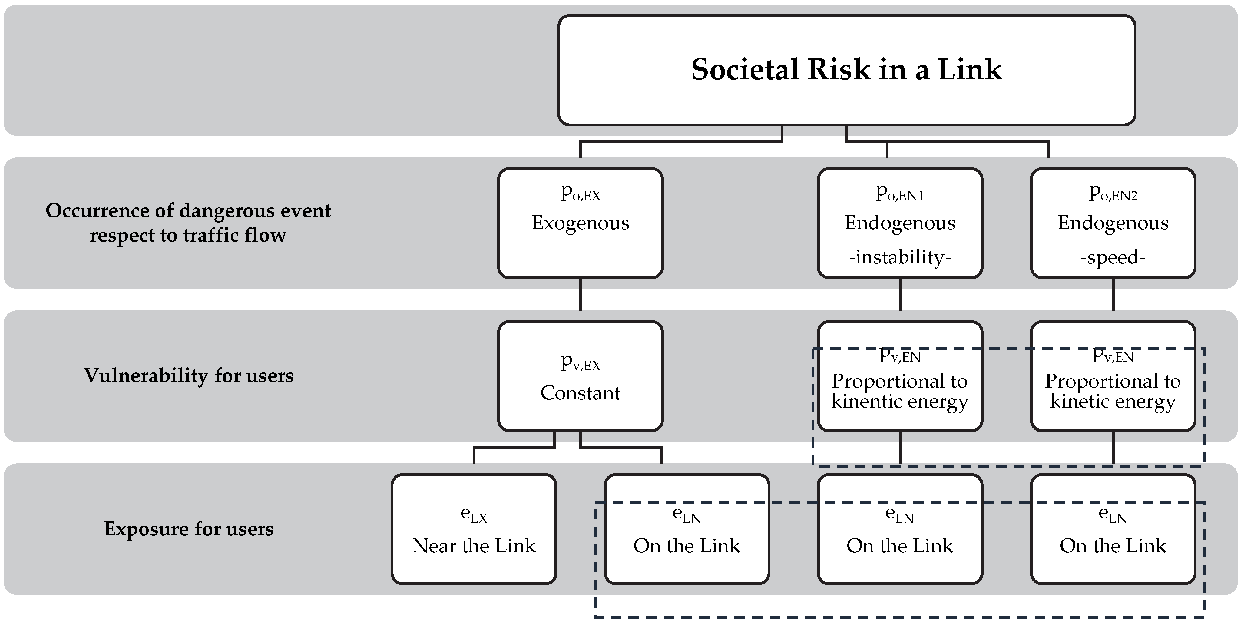
Figure 1. Proposed model (adapted from Vitetta) [20].
Futuretransp 05 00150 g001
Figure 2. Speed ratio y(x) vs. degree of saturation x, urban (left) and extra-urban (right) settings: deterministic risk analysis.
Futuretransp 05 00150 g002
Figure 3. Risk index z(x) vs. degree of saturation x, urban (left) and extra-urban (right) settings: deterministic risk analysis.
Futuretransp 05 00150 g003
Figure 4. Speed ratio y(x) vs. degree of saturation x, urban (left) and extra-urban (right) settings: stochastic risk analysis.
Futuretransp 05 00150 g004
Figure 5. Risk z(x) vs. degree of saturation x results, urban (left) and extra-urban (right) settings: stochastic risk analysis.
Futuretransp 05 00150 g005
Table 1. Glossary of symbols and parameters.
Symbol/TermDescription
TSpeed random variable
VTravel time random variable
ηShape parameter of the gamma and inverse gamma distribution
θTScale parameter of the inverse gamma distribution
θVScale parameter of the inverse gamma distribution
xDegree of saturation (dimensionless), ratio between flow and capacity
ySpeed ratio (dimensionless), ratio between speed and free flow speed
Table 2. Reference parameter values.
ParameterUrbanExtra-Urban
v0 [km/h]60120
fMAX [veic/h]20002000
a20.3
b24
β0.010.01
c = β · v00.61.2
Table 3. Reference parameter values for elasticity.
Saturation Level xRisk Index z(x)Parameter cElasticity εc
0.20.0150.85−0.42
0.50.0380.85−0.67
0.80.0210.85−0.31
Disclaimer/Publisher’s Note: The statements, opinions and data contained in all publications are solely those of the individual author(s) and contributor(s) and not of MDPI and/or the editor(s). MDPI and/or the editor(s) disclaim responsibility for any injury to people or property resulting from any ideas, methods, instructions or products referred to in the content.