Out of Alignment: Fixing Overlapping Segments in German Car Classification Through Data-Driven Clustering

Abstract

The passenger car market has experienced a radical shift: the rise of SUV, crossover vehicles, but also Battery Electric Vehicle (BEV) and Plug-In Hybrid Vehicle (PHEV), has blurred the borders between traditional vehicle segments as well as body types, resulting in reduced applicability of conventional taxonomies of vehicle types. This study aims to provide an overview of the vehicle market by proposing a new, machine-learning-based segmentation of the entire German vehicle fleet covering the past years. We merge over 40 million registered vehicles with a technical specifications database and apply data-mining techniques to derive an improved market segmentation. We demonstrate that unsupervised learning techniques, specifically Ward and k-means clustering, yield clusters with enhanced separation, clarity, and practical usability. Clustering was applied to both raw technical features and engineered features designed to capture aspects of economy, ecology, usability, and performance. The silhouette scores can reach 0.19, a significant increase over the +0.05/−0.05 scores of the existing vehicle segments or chassis types.

1. Introduction

The global ambition to tackle climate change has led to a renewed focus on the transportation sector [1]. Further, on national levels, countries have developed goals to achieve the overall reduction targets, crafting laws and regulations to make their ambition binding [2]. Within the transportation sector, road-based transportation accounts for the majority of greenhouse gas emissions; at the same time, its decarbonization lags behind [3,4,5]. Crafting effective and efficient polices is promising to reduce Greenhouse Gas (GHG)-emissions in the long run; however, it requires a profound understanding of the holistic transportation ecosystem [6,7,8,9]. As passenger car fleets consist of a wide range of different vehicles, clustering them into manageable subgroups is used to simplify the analysis and communication of findings to the public and parties of interest. Necessarily, the feasibility and precision of current approaches are critical to the validity of the derived findings. Current methods often rely heavily on predefined categories, such as vehicle class or chassis type, which can introduce inconsistencies and variations in key parameters across vehicles within the same segment. These deviations hinder the comparability of vehicles and limit the effectiveness of segmentation for certain analytical tasks. To illustrate this, the Ferrari Purosangue, the Toyota Aygo X, and the Mercedes-Benz Maybach GLS 600 are all classified as SUVs, even though their technical characteristics differ significantly (e.g., the Aygo has a curb weight of 1015 kg and the Maybach GLS a curb weight of 2825 kg). Using weight as a proxy for consumption, which is an important characteristic regarding their environmental performance, the practical usability is questionable.

In this paper, we propose a novel, data-driven approach that focuses exclusively on the technical properties of vehicles for segmentation and classification. Our methodology is built upon a dataset from the ADAC database, covering vehicle specifications from the years 2019 to 2025. By employing both raw and engineered features, we perform clustering on the data to uncover inherent groupings that are statistically more comparable than traditional vehicle categories. This approach allows for the identification of more consistent vehicle segments, free from the biases introduced by conventional segmentation keys.

To achieve this, we first perform data merging and preprocessing steps, followed by feature selection and engineering to enhance the predictive power of the dataset. The resulting feature sets are fed into clustering algorithms, which generate novel vehicle clusters based solely on technical characteristics. These clusters not only improve statistical comparability but also provide valuable insights for future vehicle categorization, especially in contexts where technical performance is the primary consideration.

Our work contributes to the growing body of research in data-driven vehicle market research, offering a new framework that can be adopted by academic researchers, commercial organizations, and public authorities seeking to adapt to the changed reality of the vehicle market. The remainder of this paper is organized as follows: Section 2 reviews related work in the field, Section 3 describes the dataset and methodology in detail, Section 4 presents the results of our clustering experiments, and Section 5 discusses the implications of our findings.

2. State of the Art

Vehicles can be categorized in different ways. On the highest level, the vehicle classes N, M, L, etc., are set according to Regulation 168/2013 and Directive 2007/46/EC by the European Union [10,11]. Within the M class (passenger vehicles), it is further differentiated into M1, M2, and M3, while M1 is of special interest for this study. M2 (>8 passengers, ≤5 $\mathrm{t}$) and M3 (>8 passengers, >5 $\mathrm{t}$) are types of buses out of this publication’s scope. Besides the classic M1 segment, M1G describes vehicles that are dedicated to off-road use. Such vehicles need to be approved by 2007/46/EG or 2018/858/EG and are listed as M1G [10,12]. Without this approval, vehicles with “off-road characteristics” are usually labeled as Sport Utility Vehicle (SUV). Older vehicles (before 1990) as well as vehicles without proper FIN are listed as motorhomes or others. Regarding passenger cars, which are commonly used for individual motorized mobility and everyday use, there are several subsections. The European Commission differentiates them based on the court decision between Hyundai and Kia in 1999 [13]. With this, the first differentiation was set, dividing the passenger vehicle market into nine segments (A: mini cars, B: small cars, C: medium cars, D: large cars, E: executive cars, F: luxury cars, S: sport coupés, M: multi-purpose cars, and J: sport utility cars (including off-road vehicles)) [13].

As one of the biggest lobby groups regarding vehicles in the EU, the European Automobile Manufacturers’ Association (ACEA) also uses certain segmentation for its communication. Their classification is similar to the one introduced by the EU in 1999. However, it does not cover sport coupés and refers to SUV rather than sport utility cars [14]. The EURO NCAP classification uses different classes, distinguishing between family cars, SUV, MPVs, Vans, and some more, all in different sizes from small to large [15]. The ICCT mentioned their classes in a report regarding a Brazilian vehicle study. In this, they state eight different passenger car classes (subcompact, compact, medium, large, sport, off-road, SUV, and minivan) [16] Other than ACEA and the EURO NCAP, they provided the technical characteristics used to classify vehicles. For this purpose, they use the system power in $\mathrm{k}\mathrm{W}$, the power-to-curb-mass ratio, the area of the vehicle, and auxiliary information (e.g., off-road vehicles need to have an all-wheel drive function, minivans need to provide between six and twelve seats). The SUV definition is borrowed from a classification according to the Brazilian automotive marketing company ADK [16].

In Germany, the Kraftfahrt-Bundesamt (KBA) is the official institution covering topics across the transportation sector. For passenger cars, they differentiate 13 segments: minis, small cars, compact cars, mid-class, upper-mid class, upper class, SUV, off-road vehicles, sports cars, minivans, large vans, utilities, and mobile homes [17]. These segments are used for enhanced comparability, using optical, technical, and market-specific characteristics, which are not necessarily included in type certification documents. Further, according to the KBA, $M1$ vehicles can be divided by certain chassis types such as sedan, hatchback, station wagon, coupé, convertible sedan, commercial vehicle, and passenger car pickup. Moreover, special-purpose vehicles are identified, such as mobile homes, ambulances, emergency vehicles, hearses, bulletproof vehicles, wheelchair accessible vehicles, and others. Finally, it is differentiated whether a vehicle has an open or closed chassis, as a necessary characteristic for a convertible car [18]. Staying in Germany, the Allgemeiner Deutscher Automobil-Club (ADAC) represents one of the most important German automotive institutions. Contrary to public authorities, the ADAC is a private automobile association, representing the interests of its members [19]. Similar to the KBA, the ADAC defines a segmentation of passenger cars; however, the segments and chassis variants differ from those the KBA uses. According to an e-mail message from the ADAC, seven different segment types are covered: micro cars, mini cars, small cars, lower middle class, middle class, upper middle class, and upper class. Further, the chassis variants are divided into 15 different types: hatchbacks, notchbacks, station wagons, coupés, convertibles, roadsters, vans, SUV, off-road vehicles, high-roof station wagons, small transporters, transporters, pickups, buses, and motorhomes [20]. For the classification parameters, such as length, width, height, wheelbase, average engine power, and corresponding basic version purchase prices are used. These criteria are compared with the average values of the corresponding chassis form with the existing segments in Germany. This decision is not influenced by third parties, according to a representative from the ADAC. Lastly, they state a dynamic classification always with respect to the actual available vehicle alternative on the current market.

Related Work

Using vehicle classes as segmentation is commonly used in studies covering fleets of vehicles. While some challenge the classes themselves, they are usually taken as they are and used to evaluate certain parts of a fleet. In the following, we focus on work that targets the classification method itself or proposes a novel approach to cluster existing vehicles. Vehicle and automotive market segmentation has been carried out using technical parameters [21,22,23,24,25,26,27,28,29,30] and user behavior [27,31,32,33], using data-driven approaches such as unsupervised learning models, often benchmarked their results against expert groups.

Perr-Sauer et al. [23] proposed a data-driven clustering approach, as they criticized the need for expert knowledge when crafting custom features for clustering. They combined fleet data with geodata and conducted a two-approach study evaluating hand-crafted features and automatically extracted features, stating comparable results. This indicates that a data-driven approach is potentially feasible for clustering vehicles. However, as their study focused on commercial vehicles driving in the United States, the transferability is questionable.

Niroomand et al. [26] noted the need for a novel approach to segment vehicles. They introduced a Fuzzy C-means and a k-means approach, showing promising results regarding the performance of the classifiers. In another study, Niroomand et al. [24] investigated a Semi-Supervised Fuzzy C-means approach to cluster passenger cars based on registration data of Switzerland. They evaluated their results against expert classification and found a better correlation compared with other unsupervised approaches. In 2022, Niroomand et al. [25] used their previously mentioned approach to analyze inter- and intra-class deviations of known vehicle segmentations with respect to ${\mathrm{CO}}_2$-emissions of the investigated vehicles. They found that within known classes, ${\mathrm{CO}}_2$-emission shows especially high variance, and further stated a potential to effectively reduce emissions by taking these variabilities into account. While all three studies show the need for novel segmentation approaches and partially mention ideas towards this (e.g., dividing vehicle classes into SUV and non-SUV), a concrete suggestion is not found in their studies. Nevertheless, they show the potential of data-driven approaches to tackle fuzzy state-of-the-art classifications of the current passenger car fleet. In 2024, Niroomand and Bach [29] used their proposed Semi-Supervised Fuzzy C-mean approach to predict average mileage values and challenged their results with a polynomial classifier. Finally, they followed up with a study extending their work with machine learning approaches, namely a Deep Fuzzy C-means model, a Support Vector Regression, and a Random Forest approach. They used their models to show their feasibility to predict engine performance as well as the environmental impact. Again, they stressed the need for adapting the state-of-the-art classification of passenger cars [30]. Vaiti et al. [28] used historical data collected via the OBD-II interface of vehicles in Canada. They propose five different vehicle classes reflecting different environmental performances. While they identify clusters and compare them to the original vehicle segments, they are limited by six features, missing potentially important features such as size and weight dimensions. Yet, they focus on Internal Combustion Engine (ICE) related features, such as cylinder size and fuel type (regular or premium gasoline, and diesel), neglecting electrified vehicles like BEV or PHEV. Nazari et al. [27] reviewed clustering strategies for electric vehicles, extending their scope to include infrastructure, user behavior, and battery characteristics. Their results underline the need for further research on the promising use of clustering approaches to segment vehicles, especially in the context of electric vehicles. Ardiansyah et al. [33] used k-means clustering for a market segmentation study for Wuling vehicles in Indonesia. They used survey data to classify different customer groups, showing another use case utilizing a data-driven approach to obtain valuable insights in the automotive world. Elser et al. [22] used Fuzzy C-means clustering on PCA-reduced technical features to segment the Swiss vehicle fleet from 1995 to 2022. Their results show shifting vehicle characteristics over time and highlight the limitations of static classifications, supporting the motivation for our work. They demonstrate this with a fixed number of clusters. To elaborate on that, we investigate the influence of the number of clusters on separation. In a previous work, Schockenhoff et al. [31,32] proposed their customer-oriented concept assessment tool to utilize certain technical parameters to create user-related features. While they provide a user-friendly approach to compare multiple passenger cars, they neither take them into perspective with existing vehicle classes nor do they extend their concept to develop a novel segmentation approach.

Summarizing the mentioned prior studies, we have identified several limitations. First, we notice a high reliance on state-of-the-art segmentations, which do not reflect the changing market conditions, especially regarding the increasing numbers of electric and hybrid-electric vehicles [21,22,23,24,25,26,27,28,29,30]. Second, the transferability to the German market is questionable, as the studies relate not to passenger cars [23] or other areas of investigation [22,23,28,33]. Lastly, while new approaches are presented, especially by Niroomand and Elster [22,24,25,26,29,30], they used a solely data-driven approach, missing the need for understandability and comprehensiveness of non-experts in order to make the proposed cluster usable.

In this article, we examine the current vehicle classes regarding their usefulness in differentiating between passenger cars. This study uses merged fleet data from the KBA with technical data from the ADAC database. Together with data-driven approaches to preprocess and later cluster the vehicle fleet we use, we compare two clustering methods with two feature selections with different cluster sizes. Raw and engineered features are extracted and used for a k-means clustering and a Ward clustering. With both approaches, we can obtain novel vehicle classes challenging the status quo, addressing the practical implementation currently missing in the field of research. We seek to contribute to the understanding of current classification weaknesses, proposing a novel approach that improves the clustering performance. Using multiple approaches, we redefine current vehicle clusters to obtain more meaningful and differentiable segments. By respecting the rise of electrified vehicles, we tend to eliminate the existing fuzziness of segments defined by out-of-date approaches. Moreover, this work proposes a framework for developing clusters using data-driven approaches and presents reasonable clusters. We show clearly how this approach can be used for different applications depending on the use case. Applying this to fleet-level data bridges gaps in current research and provides valuable insights for institutions utilizing vehicle classes.

The main contributions of this paper can be summarized as follows:

• Illustration of the current vehicle classification performance
  Using Principal Component (PC)-analysis and silhouette scores to determine the fuzziness of the state-of-the-art classification.
• Presentation of a novel segmentation approach
  Demonstration of a data-driven methodology utilizing raw and engineered features.
• Evaluation of the identified cluster performance
  Demonstration of the efficacy of the proposed methodology for the passenger car fleet in Germany.

3. Data

3.1. Data Sources

To obtain the necessary data for this study, three main sources were used and combined to create a comprehensive and representative vehicle database for the German automotive market. The KBA provides publicly accessible data on the vehicle market, including registration and stock data.

Specifically, data on the total fleet in Germany by manufacturer identifier/type identifier (Hersteller-Schlüsselnummer/Typ-Schlüsselnummer) (HSN/TSN) tuples is available for the years 2019 to 2024 [34]. This forms the foundation of the dataset, offering yearly vehicle stock counts for each HSN/TSN pair.

To enrich the dataset with technical specifications, the HSN/TSN tuples were matched to entries in the ADAC Vehicle Catalog [20]. This source includes detailed technical information such as energy consumption, gross vehicle weight, and vehicle dimensions, along with 218 other technical parameters for virtually all cars sold in Germany.

Finally, the Gesamtverband der Versicherer (GDV) provides information on vehicle type classes used in insurance classification [35]. Although insurance premiums are influenced by both vehicle and regional factors, only the model-specific insurance classification was considered in this study.

We paid attention to not using time-sensitive data, if possible, without neglecting necessary data. However, no auxiliary characteristic was found for the purchase price. To account for inflation, the Customer Price Index (CPI) was used to compare purchase prices of the vehicles at their market introduction with today’s price level.

The corresponding data was obtained from the World Bank [36], with the Destatis data for the year 2024 [37]. For the years 1956 to 1959, a CubicSpline extrapolation was used based on the existing data ranging from 1960 to 2024.

In total, we identified 17,995 models with 43,160,306 registered units with enough attributes to be processed. This constitutes 87% of Germany’s total vehicle stock [38].

3.2. Data Exploration

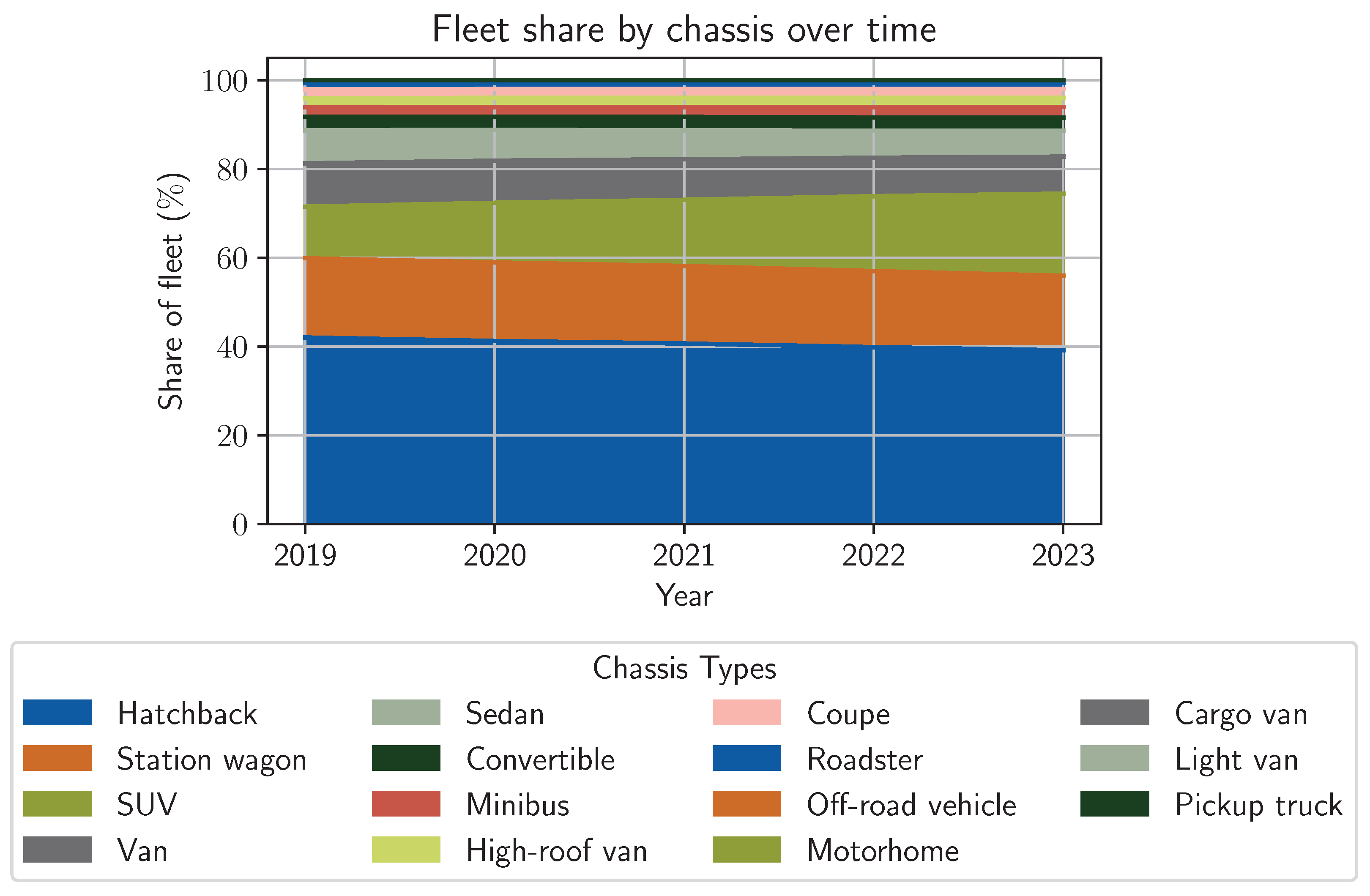
In this section, we analyze the combined dataset from the KBA and the ADAC, focusing on the distribution and evolution of the vehicle fleet in Germany. This preliminary exploration serves as a foundation by illustrating key structural patterns in the technical characteristics of the vehicles. In general, fossil-fueled vehicles account for the majority of the German fleet, with 29.9% for diesel and 66.6% for petrol-powered vehicles. While electrified vehicles show a significant increase since the start of the surveyed period in 2019, their share only accounted for 0.9% for PHEVs and 2.2% for BEVs in 2023. (Delta to 100%: other fuel types, e.g., H₂ or LNG/CNG excluded from further analysis). Regarding vehicle classes (ADAC), the fleet composition remained stable between 2019 and 2023. In contrast, chassis types showed multiple shifts, illustrated by Figure 1. Where most types remained constant, a significant shift towards SUV can be observed, rising from 11.6% in 2019 to 18.5% in 2023. Further, mini-buses gained 0.5%.

This increase is mainly caused by the reduction in conventional chassis types, such as sedans, vans, and station wagons, while other types showed small or no changes.

Besides the general fleet composition, the technical characteristics also changed. Figure 2 illustrates deviations in the average of the parking space ($\mathrm{length}\times \mathrm{width}\times 1.1$), given in ${\mathrm{m}}^2$ the curb mass, given in $\mathrm{k}\mathrm{g}$, and the consumption, given in $\mathrm{k}\mathrm{W}\mathrm{h}/100 \mathrm{k}\mathrm{m}$. The shaded areas visualize the standard deviation for all cars of a certain vehicle class.

It shows that the parking space remains almost constant for the vehicle classes, with a clear distinction between them. Only luxury and upper mid-size vehicles overlap for this characteristic. The order in magnitude aligns with the semantic interpretation for the vehicle classes. Regarding the curb mass, a general increase can be observed. All vehicle classes show an increase in curb mass since 2019. Further, the standard deviation is bigger, resulting in an overlap of the curves, which makes it more difficult to distinguish between the vehicle classes. The highest increase shows small cars with $8.2$%, followed by lower mid-size cars with $5.6$% and mid-size cars with $5.1$%. Upper mid-size and luxury vehicles show a lower increase of $1.1$% and $0.8$%, respectively.

The consumption values for all cars were corrected as explained in Section 4.1, allowing for fair comparability between different energy types such as electricity, fossil fuel, and a mix of both (PHEV). In general, consumption values have decreased over the survey period. We discovered that across fuel types, consumption values tend to decrease while showing an overlapping variance band, making fuel type-based conclusions fuzzy. Mini cars and mid-size cars show the largest reduction with $-36.4$% and $-20.8$%. Luxury cars have lowered their average consumption by $-2.6$%. Microcars show an increase by $4.1$%; however, the number of vehicles within this class is significantly lower than others, making it more prone to statistical sensitivities. It should be noted that, compared with the other two technical characteristics, the deviation within a class is significantly higher, led by luxury and upper mid-class vehicles with values of $30.1$ and $23.0$. This indicates a high variability and highly diverse performance within the same vehicle class. Besides these two, all other vehicle classes also show an increase in their standard deviation; this observation seems to become more relevant over time.

4. Methodology

Figure 3 provides an overview of the implemented data pipeline. The three main steps include data preprocessing, pattern mining, and evaluation. Preprocessing accounts for data cleaning, imputation, and feature engineering. The selected clustering algorithms are applied in the pattern mining step. For quantification of the results, Key Performance Indicator (KPI)s are calculated in the evaluation step. Notably, the clustering is performed on both the raw features and the engineered features in parallel to allow for a comparison of the results between not only the legacy clusters but also both feature sets.

4.1. Data Preprocessing

To handle missing values, k-NN imputation was used. This method is based on the assumption that similar data points are likely to have similar values [39]. This assumption is particularly relevant in the context of vehicle data, as highly similar vehicles like different trims of the same model can be used to impute each other’s missing values. It was decided against mean or median-based imputations as these methods, compared with k-NN imputation, could lead to stronger loss of local structure in the data [39].

To account for different scales of the features, the data was normalized using a standard scaling method. This method transforms the data to have a mean of zero and a standard deviation of one. This normalization was used for both raw and engineered features.

4.2. Feature Engineering

In this study, we use both raw features from the technical data and engineered features. The former consists of the raw data of the ADAC-database combined with the corresponding amount of vehicles in stock from the KBA-data. We aim to leave the raw data untouched wherever possible; however, some data needed to be adjusted to allow for comparison over the inflation and different fuel types. As stated in Section 3, we found that purchase prices are not comparable over time due to inflation. As the inflation rate is not constant, we use CPI-data to account for the variability of inflation rates. Starting with the original price $P_{\mathrm{original}}$ the adjusted price $P_{\mathrm{adjusted}}$ is calculated as

$$P_{\mathrm{adjusted}}=P_{\mathrm{original}}\times {\displaystyle \frac{{\mathrm{CPI}}_{\mathrm{now}}}{{\mathrm{CPI}}_{\mathrm{then}}}}.$$

(1)

Furthermore, we introduced an adjusted consumption value and an adjusted range value to allow for comparison between different fuel types. Consumption values calculated in kW h km⁻¹ unify the units for BEV, PHEV, and fossil-fueled vehicles. If range values are not directly provided in the database, it is calculated using consumption and fuel tank size and/or battery capacity values. Consumption values for the PHEV are corrected by the observed deviation from their data sheet values. A study from the European Commission regarding real-world consumption identified an excess of $254.1$% for D-PHEV and $326.0$% for P-PHEV [40]. We use this factor combined with the ratio between D-PHEV and P-PHEV (8%/92%) to obtain a more realistic emission factor for PHEVs.

Equations (2) and (3) show how these values are calculated. For the adjusted consumption, first, the different measuring cycles are harmonized: WLTP, NEDC, Drittelmix, or None at all. The data sheet consumption C is used and normalized using conversion factors $f_{\mathrm{logic}}$. With $\mathrm{L}$ to $\mathrm{k}$$\mathrm{W}$$\mathrm{h}$ conversion factors $c_{\mathrm{conversion}}$, all consumption values are finally given in kW h km⁻¹. With the now calculated adjusted consumption values, the adjusted range can be calculated. For this, the adjusted consumption $C_{\mathrm{adjusted}}$ is simply divided by the tank size $V_{\mathrm{tank}}$.

$$\begin{array}{cc}\hfill C_{\mathrm{adjusted}}& ={\displaystyle \frac{C\times c_{\mathrm{conversion}}}{f_{\mathrm{logic}}}}\hfill \\ \hfill f_{\mathrm{logic}}& =\left\{\begin{array}{cc}1\hfill & \mathrm{if}{C}_{\mathrm{WLTP}}\mathrm{is}\mathrm{available}\hfill \\ 0.9\hfill & \mathrm{else}\mathrm{if}{C}_{\mathrm{NEDC}}\mathrm{is}\mathrm{available}\hfill \\ 0.8\hfill & \mathrm{else}\mathrm{if}{C}_{\mathrm{Drittelmix}}\mathrm{is}\mathrm{available}\hfill \end{array}\right.\hfill \\ \hfill c_{\mathrm{conversion}}& =\left\{\begin{array}{cc}9.96\hfill & \mathrm{if}\mathrm{motor}\mathrm{type}\mathrm{is}\mathrm{Diesel}\mathrm{or}\mathrm{Diesel}\mathrm{Hybrid}\hfill \\ 8.76\hfill & \mathrm{if}\mathrm{motor}\mathrm{type}\mathrm{is}\mathrm{Otto}\mathrm{or}\mathrm{Otto}\mathrm{Hybrid}\hfill \\ 1\hfill & \mathrm{if}\mathrm{the}\mathrm{motor}\mathrm{type}\mathrm{is}\mathrm{BEV}\hfill \end{array}\right.\hfill \end{array}$$

(2)

$$\begin{array}{cc}\hfill R_{\mathrm{adjusted}}& =\left\{\begin{array}{cc}{\displaystyle \frac{V_{\mathrm{tank}}}{C_{\mathrm{adjusted}}}}\hfill & \mathrm{if}\mathrm{ICE}\mathrm{and}\mathrm{tank}\mathrm{size}\mathrm{are}\mathrm{given}\hfill \\ {\displaystyle \frac{V_{\mathrm{tank}}}{C_{\mathrm{adjusted}}\times f}}\hfill & \mathrm{if}\mathrm{PHEV}\mathrm{and}\mathrm{tank}\mathrm{size}\mathrm{are}\mathrm{given}\hfill \\ \mathrm{WLTP}\mathrm{range}\hfill & \mathrm{for}\mathrm{electric}\mathrm{vehicles}\hfill \\ {\displaystyle \frac{L_{\mathrm{ft},\mathrm{class}}}{C_{\mathrm{adjusted}}}}\hfill & \mathrm{if}\mathrm{tank}\mathrm{size}\mathrm{or}\mathrm{battery}\mathrm{capacity}\mathrm{is}\mathrm{not}\mathrm{given}\hfill \end{array}\right.\hfill \\ \hfill \mathrm{with}f& =\left\{\begin{array}{cc}3.26\hfill & \mathrm{if}\mathrm{hybrid}\mathrm{fuel}\mathrm{type}\mathrm{is}\mathrm{Diesel}\hfill \\ 2.63\hfill & \mathrm{otherwise}\hfill \end{array}\right.\hfill \end{array}$$

(3)

To calculate ${\mathrm{CO}}_{2-\mathrm{eq}.}$ emissions per kilometer, the consumption values were multiplied by the emission factors of the fuels, which are listed in

Table 1. Emission factors for petrol, diesel, and electricity regarding Tank-to-Wheel (TtW), and Well-to-Wheel (WtW).

Fuel Type	TtW-Value	WtW-Value	Unit	Source
Diesel	2.95	3.08	$\mathrm{kg}{\mathrm{CO}}_{2-\mathrm{eq}.}/\mathrm{L}$	[41]
Petrol	2.60	2.73	$\mathrm{kg}{\mathrm{CO}}_{2-\mathrm{eq}.}/\mathrm{L}$	[41]
Plug-in Hybrid	2.33	2.45	-	[40,42]
BEV	0	0.427	$\mathrm{kg}{\mathrm{CO}}_{2-\mathrm{eq}.}/\mathrm{kWh}$	[42]

. In all propulsion types, to account for upstream emissions, we apply the Well-To-Wheel approach to account for fuel production emissions that happen before energy conversion in the car.

Besides the (adjusted) raw features, engineered features were also used. We defined four different scores targeting different customer values: performance, usability, economic, and ecological. The choice of these four aggregated features leans on the current methodology of vehicle classification, in which vehicles are clustered using technical specifications such as (see introduction here). Combined with methods from literature [31,32], several technical characteristics can be combined to form a customer value, such as acceleration and max speed, into a performance indicator.

Table 2. Feature Breakdown: Components, Min–Max Values for the Sigmoid Normalization, and Weights.

Feature Name	Component	Min–Max	Weight
Performance	Acceleration	[18, 2.5]	0.5
	Max Speed	[150, 300]	0.5
Usability	Number of Seats	[2, 9]	0.25
	Trunk Volume	[98, 784]	0.25
	Adjusted Range	[0, 1000]	0.25
	Payload	[112, 778]	0.25
Economic	Adjusted Consumption	[250, 20]	0.25
	Adjusted Price	[250,000, 15,000]	0.25
	Tax	[1664, 14]	0.25
	VK	[34, 10]	0.083
	TK	[33, 10]	0.083
	HK	[25, 10]	0.083
Ecological	${\mathrm{CO}}_2$ Emission per 100 km	[300, 15]	0.5
	Adjusted Consumption	[250, 20]	0.5

shows the different characteristics used with their individual weighting factor. Further, the min and max values for the sigmoid normalization function are given. All sigmoid normalization uses the k factor 5. Equations (4) and (5) show how the final sigmoid value is calculated. Note that the min and max values are sometimes inverted (e.g., for the acceleration); lower values are treated as a better characteristic. All weights are equally distributed, while VK, TK, and HK are combined into one, representing different insurance classes for the vehicle. (VK: fully comprehensive insurance coverage TK: partially comprehensive HK: liability insurance).

$$\begin{array}{cc}\hfill \mathrm{Let}\widehat{x}& =\left\{\begin{array}{cc}0.5,\hfill & \mathrm{if}{\max }_{\mathrm{val}}={\min }_{\mathrm{val}}\hfill \\ min\left(1,max\left(0,{\displaystyle \frac{x-{\min }_{\mathrm{val}}}{{\max }_{\mathrm{val}}-{\min }_{\mathrm{val}}}}\right)\right),\hfill & \mathrm{otherwise}\hfill \end{array}\right.\hfill \end{array}$$

(4)

$$\begin{array}{cc}\hfill f(x)& =\left\{\begin{array}{cc}0,\hfill & \mathrm{if}x\mathrm{is}\mathrm{invalid}(\mathrm{e}.\mathrm{g}.,x<0\mathrm{or}\mathrm{NaN})\hfill \\ {\displaystyle \frac{1}{1+exp(-k(\widehat{x}-x_0))}},\hfill & \mathrm{otherwise}\hfill \end{array}\right.\hfill \end{array}$$

(5)

4.3. Evaluation KPI

The silhouette score is a well-established metric used to evaluate the tightness and separation of clusters [43]. It measures how similar an object is to its own cluster compared with other clusters. The silhouette score for a single data point is calculated as stated in Equation (6) [43]:

$$s_i={\displaystyle \frac{b_i-a_i}{max(a_i,b_i)}}$$

(6)

$$s_{\mathrm{avg}}={\displaystyle \frac{{\sum }_{i=1}^n{s}_i\times n_i}{\sum n_i}}$$

(7)

Here, a represents the average dissimilarity (or distance) between the data point and all other points within the same cluster, while b is the average distance between the data point and its on average closest neighboring cluster. The silhouette score ranges from −1 to 1, where a value close to 1 indicates that the data point is perfectly matched to its own cluster. A score near 0 suggests that the data point lies on the boundary between clusters, and a negative score indicates that the data point has a stronger association with its neighboring cluster than with its own. For small cluster sizes, the silhouette can be visualized and examined for each single data point. As this article examines over 20,000 car models, we will only rely on the silhouette score averaged over a whole cluster from now on.

The car models have significantly differing sales numbers $n_i$. This would translate to multiple data points at the same location in the feature space, with the same silhouette $s_i$ each. To account for this imbalance, we weight all silhouette values $s_i$ with their respective sales numbers $n_i$ to retrieve the weighted average silhouette score $s_{\mathrm{avg}}$ as presented in Equation (7). Practically, this means that a vehicle model with a higher number of sales will have more data points in the dataset, hence a stronger influence on the average silhouette.

4.4. Methods of Clustering

A suitable clustering method was chosen by exclusion, starting with the full set of clustering algorithms provided by the scikit-learn library [44]. The candidates include partitioning, hierarchical, density-based, model-based, grid-based, and representation-learning methods. The clustering algorithms were limited to those that are suitable for the data and the research objective. As every vehicle shall be assigned to a cluster, density-based methods (DBSCAN, OPTICS) were omitted as they create separate noise clusters [45], which is not desired for this task. Moreover, the additional parameters needed for density-based methods are unstable for the heterogeneous data at hand [46]. Model-based methods were also excluded as their soft-assignment [47] probabilistic cluster memberships conflict with our hard-label KPI. The goal is to assign each vehicle to a single cluster, and probabilistic memberships would not provide a single assignment and thus make it incompatible with the selected KPI. Grid-based methods are rejected for their mandatory discretization of the data, which introduces artificial boundaries in the continuous numerical data. Lastly, deep and representation-learning methods were excluded for their intransparent nature [48]. This leaves hierarchical agglomerative (Ward), and partitioning (k-means) methods as they satisfy the no-noise and hard-assignment criteria. Additionally, the option to manually specify the number of clusters in both methods [49,50] is important for the research objective, as that provides consistency for evaluation. Further, it allows for the selection of a number of clusters equal to the legacy classification, improving the comparability of the results. Lastly, their minimal hyperparameter requirements make them suitable for the heterogeneous data at hand.

The previously mentioned sales proportional up-sampling is of particular importance for the k-means method, as it is sensitive to the distribution of the data. Duplicating high-volume models proportionally gives them more weight in the clustering process. While the Ward method does not explicitly require this, it is still valid to feed in the same up-sampled data, as vehicles that share the same coordinates in the feature space are merged into a single cluster early on, keeping conceptual similarity.

5. Results

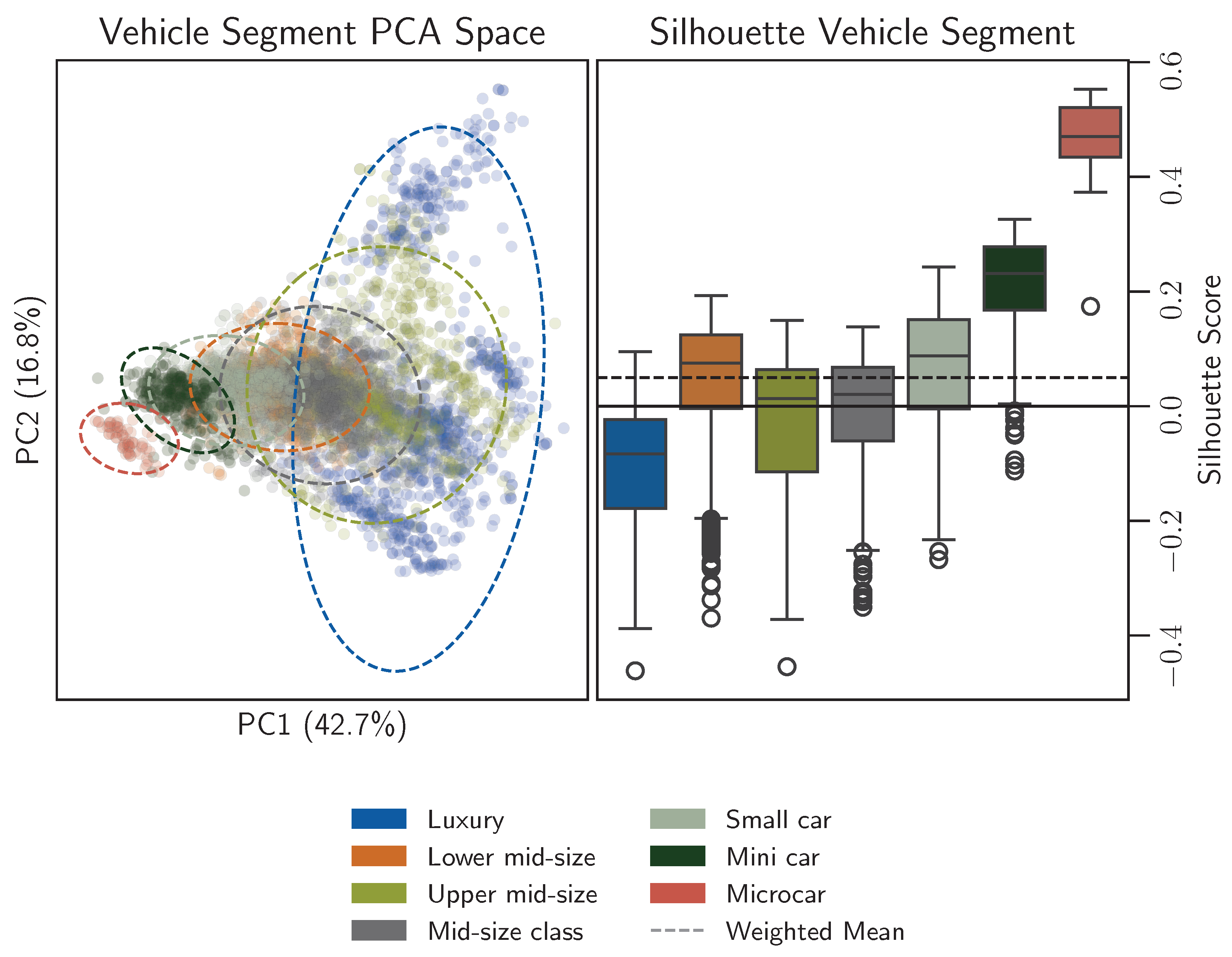
To start out, Figure 4 presents a comprehensive assessment of the status quo of the classification into vehicle segments as documented in [20]. The left plot presents the vehicle segments in the principal component space (All plots of this type are available as interactive plots on https://tumftm.github.io/passenger-vehicle-clustering/ (accessed on 17 September 2025), along with the vehicle models associated, and we highly encourage exploring them for a better understanding of the matter): The first PC on the x-axis explains $42.7$% of the variance, while the second PC is on the y-axis and contributes another $16.8$%. The data is projected into the PC1/2 space, as this provides the most informative 2D representation for the purposes of this paper.

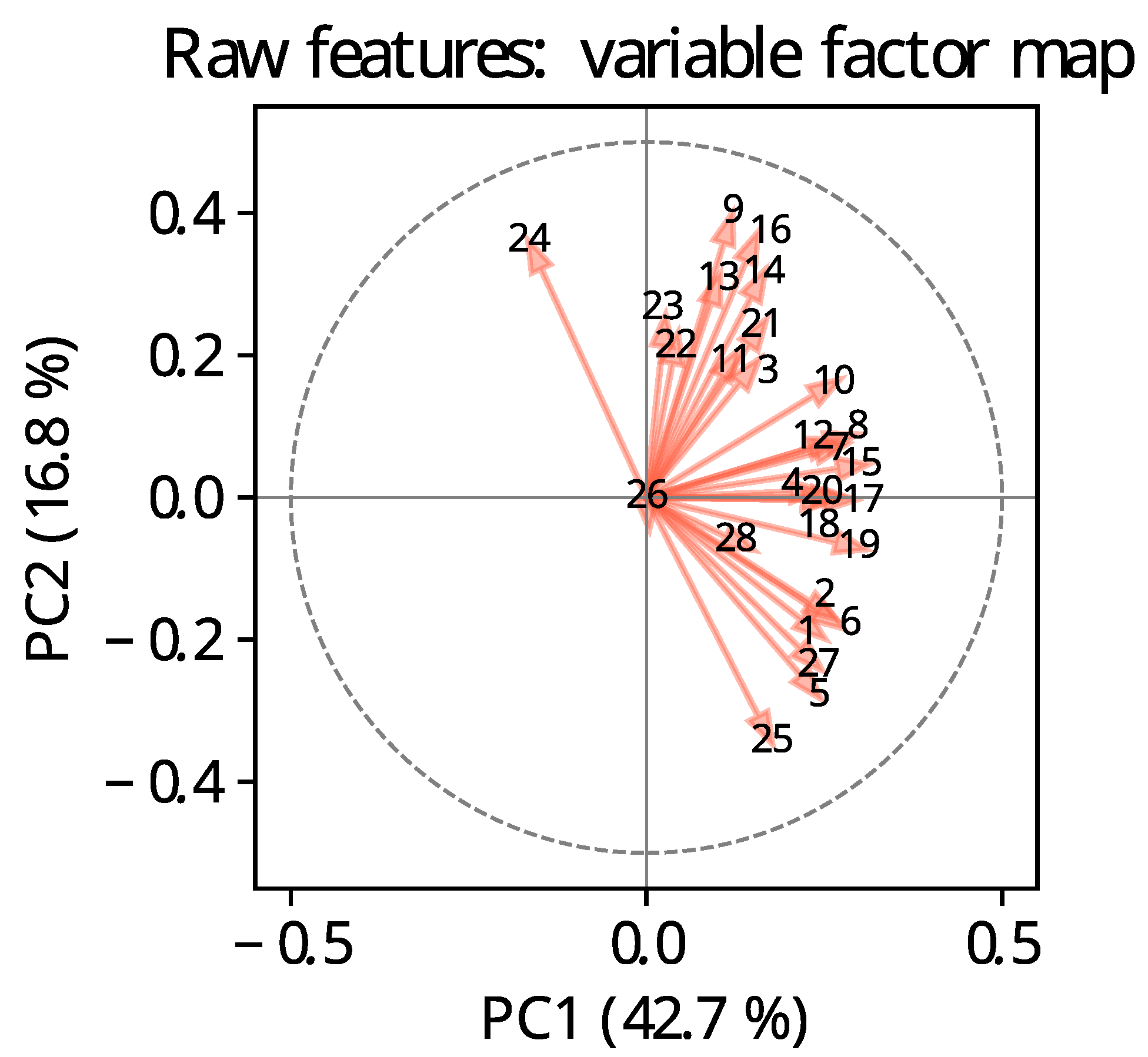
Each dot represents a vehicle model, and each ellipse indicates the 95 percent confidence region of the cluster covariance in the PC-plane. As Figure A3 in the appendix demonstrates, PC1 is strongly aligned with features like towing load, curb weight, or fuel consumption. PC2 aligns more strongly with the number of doors, the number of seats, or the vehicle height. Consequently, micro, small, and mini cars are mostly on the left, to the lower-left side of the plane, while higher segments are mostly oriented towards the right. The variance within clusters of higher segments is generally higher, as e.g., sports cars, SUV, and high-priced vans are all within the luxury segment, but are scattered widely across the PC-plane.

The right plot visualizes the silhouette values for the representatives of each cluster as box plots. The low separation quality becomes obvious, as 2 clusters have an average silhouette near zero (mid-size class, upper mid-size class), and luxury cars have a negative silhouette on average. To put this into perspective, more than 75% of luxury cars are more similar to other segments than to other luxury cars, similar to the sports version of a sedan being more similar to a sedan than an expensive SUV.

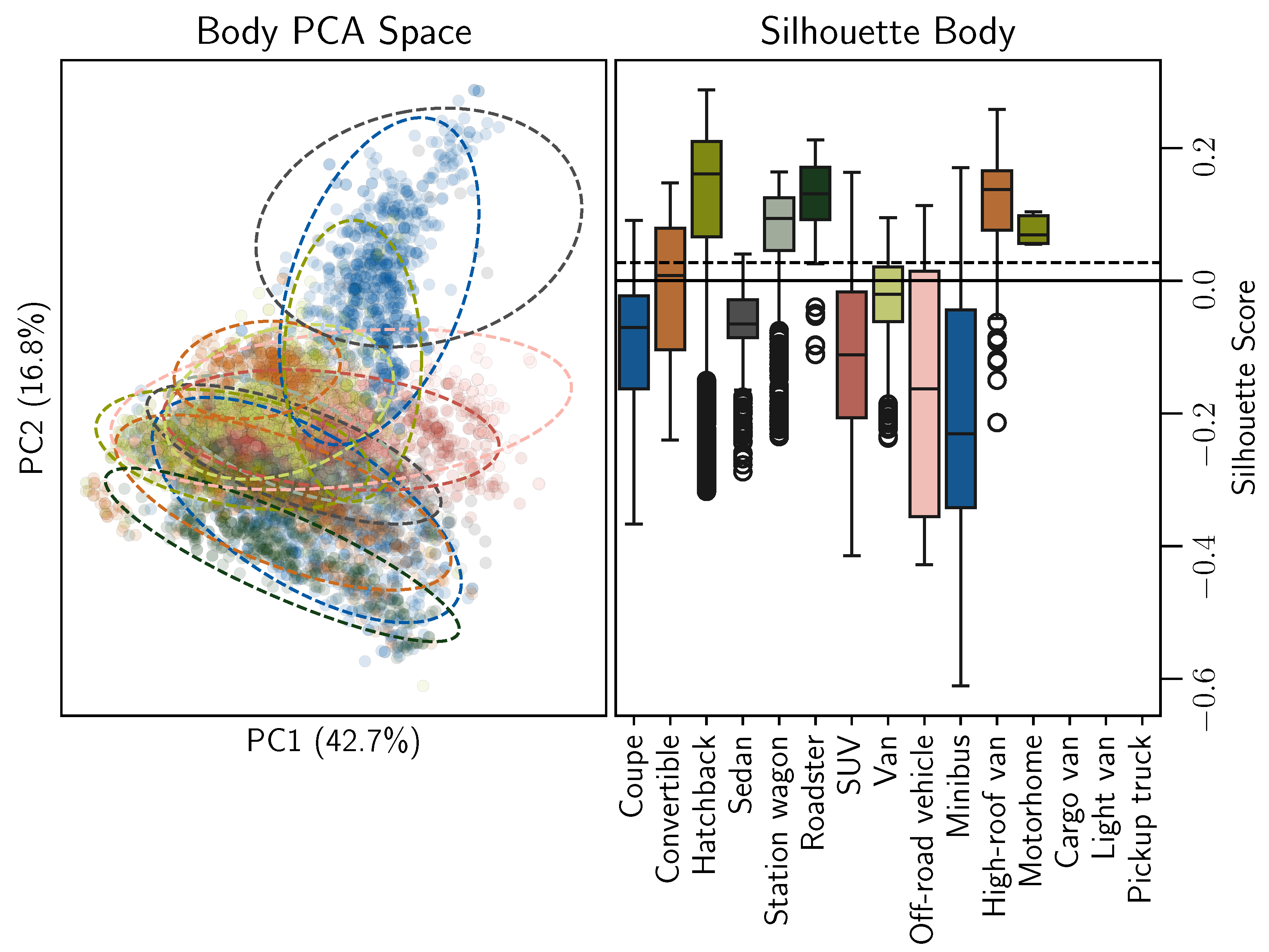
The goal of this article is to find a cluster partition that demonstrates better silhouettes quantitatively and good semantic similarity within a cluster qualitatively. For this purpose, the clustering methods presented in Section 4 are evaluated for different numbers of clusters in Figure 5. Here, the state of the art is represented by the dashed lines, indicating the silhouette of vehicle segments and vehicle chassis types evaluated in the aggregated feature space.

First and foremost, both clustering methods, k-means and Ward, on both feature sets, raw and aggregated, perform superior to the state of the art—for all numbers of clusters, our methods exhibit a higher silhouette score than the partition into segments or chassis types. The silhouette reach of the k-means and Ward clustering results reaches up to $0.31$ for two clusters and declines slightly with increasing number of clusters. A higher number of clusters generally allows for more specific labeling of the subgroups, yet a lower number of clusters increases separation. To select a specific value for further analysis, we opt for the compromise $n=7$ for two reasons: Firstly, it is equal to the number of vehicle segments, and thus maximizes comparability with the state of the art. Secondly, the k-means algorithm on aggregated features exhibits a local maximum in its silhouette here, and thus hints at an inherent partition into seven groups within the dataset.

Within the raw feature set, Ward performs superior to k-means, while k-means outperforms Ward on the aggregated feature set. We thus select both winners for closer examination in Section 5.1 and Section 5.2, but the other two results are provided in the appendix. Notably, the clusters are not related to any existing classification of vehicles anymore: to provide a descriptive and memorable working title for those clusterings, we fed 10 randomly drawn vehicles to ChatGPT version 4o. The prompt template used is documented in the appendix.

5.1. Clustering Using Raw Features

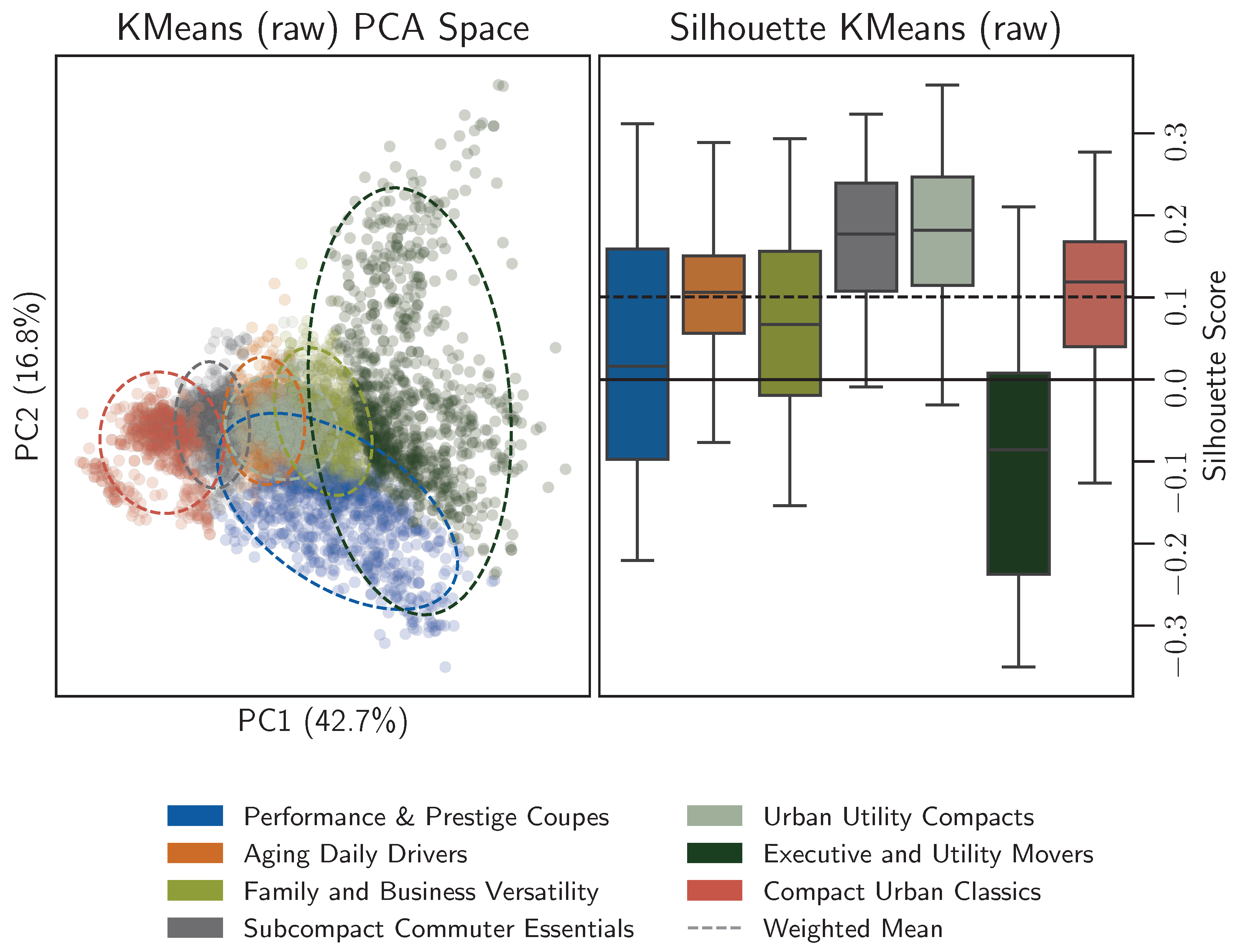
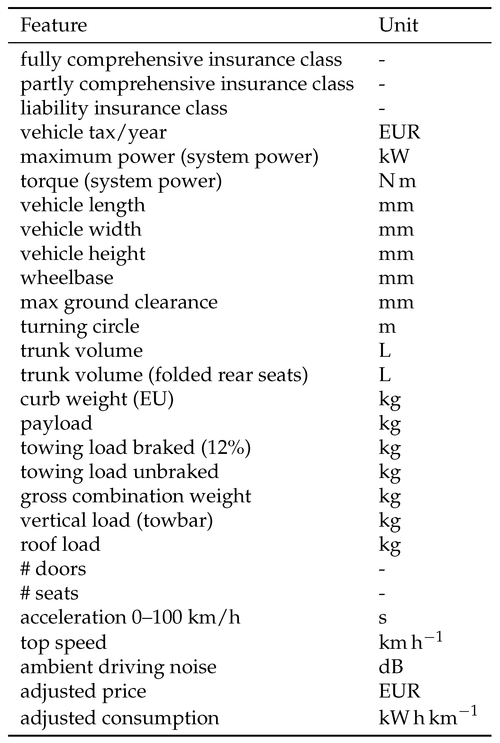
Starting with raw features listed in Figure A1, the Ward approach outperforms k-means with a silhouette score of around $0.13$ compared with $0.10$ at $n=7$. Figure 6 shows the clustering result in the PC plane in the left panel and the silhouette scores in the right. Now, all but one cluster exhibit silhouettes that are positive on average. The worst separation is observed for the All-Terrain Family Utility type (e.g., Land Rover Defender 90, Jeep Wrangler, but also VW T5 Multivan, and Peugeot Partner Kombi), which has a close proximity to Modern Commuter Workhorses and Refined Executives for Professional Mobility. Modern Commuter Workhorses holds vehicles such as a Honda Civic, Opel Zafira, and Audi A6 Avant, while Refined Executives for Professional Mobility covers cars such as Skoda Superb Combi and BMW 335i, but also a Cadillac Escalade, which is more of an outlier than a centered data point in this cluster. At first sight, these clusters are semantically similar to each other and the ellipses overlap; however, their centers are different on both PC axes.

The cluster for Elite Roadsters & Performance Icons and Aging Essentials with Everyday Appeal shows the highest average silhouette scores around $0.2$. This is plausible, as their location in the PCA space is also at the lower right and left edges, with a clearer distinction from other clusters. The semantic name for the Elite Roadsters & Performance Icons cluster makes sense when inspecting the individuals of it, mainly consisting of Porsche, Jaguar, and Mercedes-Benz AMG vehicles. Aging Essentials with Everyday Appeal contains rather small and compact vehicles such as a FIAT Panda 4×4, VW Golf, and Dacia Duster. The cluster with the highest variance is Luxury Performance Titans, as the majority of its entities are high-priced vehicles with much engine power. On the bottom part, similar vehicles compared with the Elite Roadsters & Performance Icons can be found (e.g., Porsche Panamera, Mercedes-Benz AMG SL 63). At the upper part of the cluster, bigger vehicles are located (e.g., Toyota Land Cruiser, Ineos Grenadier, and Mercedes-Benz G280 CDI). Multi-Purpose Transport Shuttles is located at the upper section of the PCplane, which aligns with the height characteristics of such vehicles (e.g., VW T4 Kombi, Mercedes-Benz Sprinter, or Citroen Jumpy Kombi) and the PC2 axis. In general, the clusters are separated quite well, apart from All-Terrain Family Utility. Comparing the clustering structure to the k-means results visible in Figure A4, the clusters are clearly distinguishable from each other, and the low-performing Executive and Utility Movers cluster is separated into two clusters.

5.2. Clustering Using Engineered Features

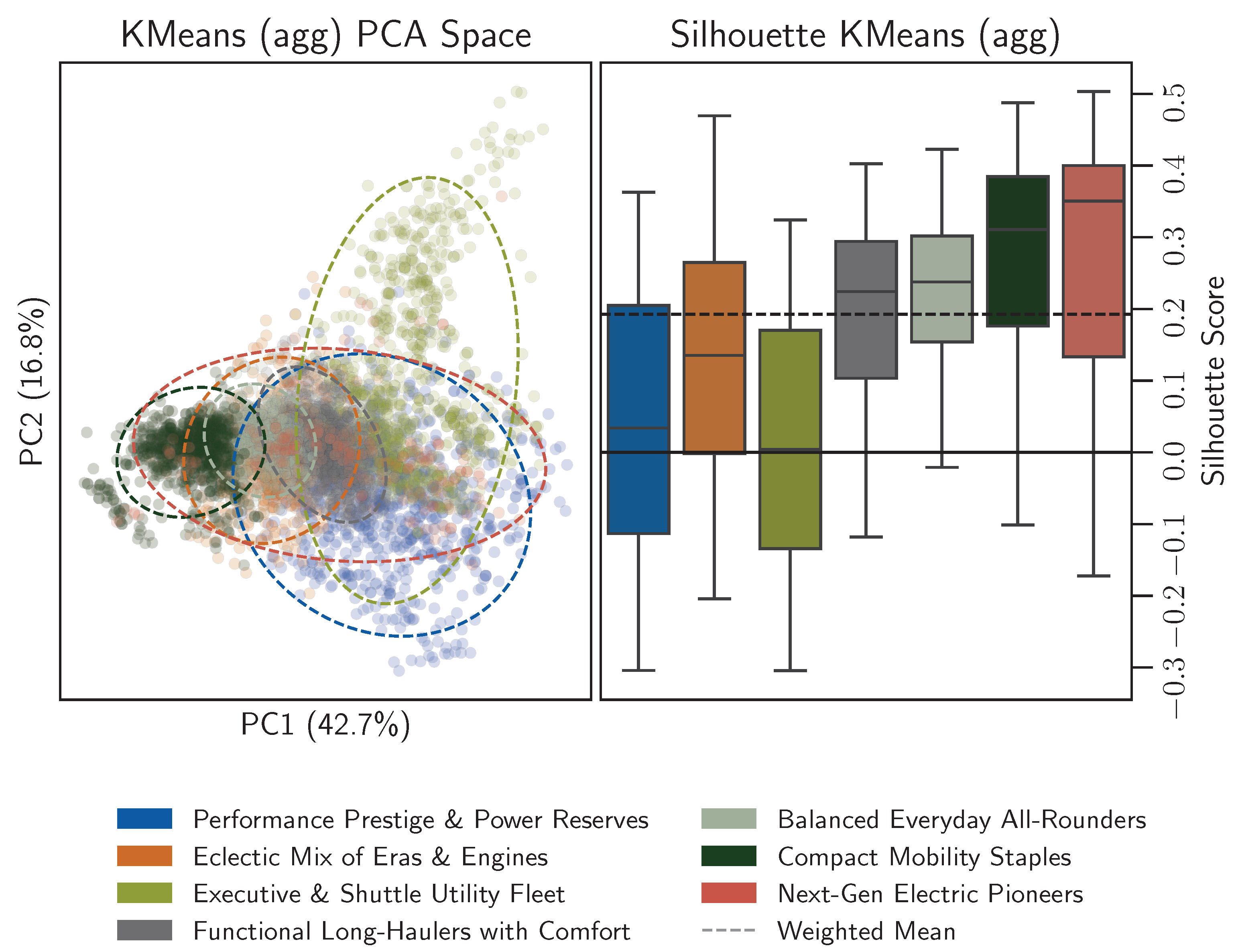
Utilizing the engineered features, described in Table 2, we compute the clusters using k-means and Ward again, yet evaluate the silhouette on the engineered feature space, too. In this context, k-means shows better performance than the Ward approach, with a silhouette score of $0.19$ vs. $0.13$ at $n=7$. These values indicate meaningful structure in the data, when compared with legacy classifications, which often yield silhouette scores close to 0, suggesting little to no separation in the technical feature space. The PC plane remains the same for comparability, but the larger variance within clusters in the plot hints at the fact that the principal components of the raw feature space do not reflect the engineered feature space ideally anymore. Yet we maintain the visualization to assure comparability with Figure 6. This is the reason that even clusters spanning the whole PC plane (Next-Gen Electric Pioneers) can maintain a good separation, as shown in Figure 7.

The Executive & Shuttle Utility Fleet has a high variance and a slightly negative average silhouette, but all other clusters are positive. Going even further, this is the first approach that ensures that 5 out of seven clusters even have non-negative lower quartiles. Analyzing single vehicles in this cluster, this variance can be explained as on the PC1 axis, almost all vehicles with a value of more than 5 are within this cluster. This area covers especially utility vehicles, e.g., VW Crafter, Mercedes-Benz Sprinter, and Ford Transit. On the lower right side, more SUV-like vehicles are located, e.g., BMW X7, Mercedes-Benz G350, and Land Rover Discovery. Centered vehicles within this cluster are a mixture of larger vehicles in general, e.g., VW Sharan, Audi Q5, and Opel Insignia. Interestingly, the Next-Gen Electric Pioneers has the highest distinction. Inspecting the distribution of the four engineered features, we observe that the ecological factor is significantly higher than in other clusters, with a mean value of $0.92$. Further, the economic factor is above average with a mean of $0.72$. Both seem plausible as BEV are superior in terms of emissions and energy efficiency, which also supports the economic performance. Moreover, the clustering algorithm found a cluster consisting only of BEV on its own without utilizing a discrete variable for this. We assume a mix of the low ecological and economic factors is responsible for this cluster. With only one outlier, a VW e-Crafter, the cluster is well described. The overall spread is more along the PC2 axis, spanning from smaller electric vehicles such as the Smart ForTwo Cabrio EQ up to large BEV such as the BMW iX M60 or the Tesla Model X Plaid.

Finally, to mention, Figure A5 has a lower silhouette score compared with the k-means approach; however, the silhouette scores from all clusters are positive, but the average values are lower. This does not necessarily mean that the clusters are less useful; rather, it indicates the need for a concise metric to evaluate the clustering performance for a real-world problem.

6. Discussion and Summary

This study shows the high variance of the state-of-the-art segmentation of the German passenger car landscape and proposes a novel segmentation approach. We combine the publicly accessible database from the KBA with the ADAC, creating a database that holds fleet size data along with technical characteristics for each vehicle. The HSN/TSN keys are used to map vehicles, allowing for easy and reproducible preprocessing. Two variants of features are derived, once a carefully selected subset of the raw features, and once engineered features that combine certain technical characteristics into more abstract features (see Section 3). First, the status quo is evaluated using the vehicle class and chassis type as clusters. Finally, utilizing the raw and aggregated features, two clustering algorithms are applied to create new clusters. For raw features, the Wardalgorithm performed better, and for the aggregated feature set, k-means performed better.

With the combination of both datasets at the beginning of the study, we encountered issues regarding the data congruence of both datasets. Within the ADAC database, the HSN/TSN key is not unique, but multiple trims of a model hold the identical key. We thus only included the basic trim of the vehicles in question; however, we lose information at this point. As the KBA database does not hold more specific details regarding certain variants, this assumption is necessary, and the information loss is inevitable. However, putting the number of appearances into account, we find that the overall coverage is good, as our dataset holds $43.2$ million vehicles. The KBA states that in 2024 $49.1$ million passenger cars were registered in Germany, which indicates a coverage rate of around 87% [38].

In terms of preprocessing, we adjusted and imputed some of the technical data, sometimes to allow for better comparability over time, such as the adjusted price values, and sometimes to allow for better comparability across different fuel types, such as the adjusted consumption values. Even though making plausible and valid assumptions regarding correction factors and inflation rates, adjusting these values introduces uncertainty to the dataset. It is yet to be evaluated how much the adjustment can contribute to reducing this and creating a fair and comparable dataset. We are aware of this circumstance and refer to future studies in this field.

The choice of clustering methods was determined through an assessment of dataset characteristics and task requirements. Given the need for hard assignments, noise-free labeling, interpretability, and no discretization, only k-means and Ward met all criteria. Both methods let us set the cluster count explicitly and require minimal additional hyperparameter tuning, making them ideal for this study. In evaluating both methods, k-means outperformed Ward on aggregated features, while Ward prevailed on the raw feature space. Feature engineering reduced dimensionality and noise, yielding more compact, convex clusters. In this setting, k-means likely outperforms Ward because its reliance on Euclidean distance implicitly assumes convex, isotropic cluster shapes. In contrast, the hierarchical agglomerative method Ward iteratively merges clusters based on variance minimization and can thus capture more complex relationships between samples. In the high-dimensional raw feature space, noisy, imbalanced, or hierarchically nested relationships are more likely to occur, which could be a reason why Ward generally excels in the raw feature space.

A strength of the method is the transition of the unsupervised learning problem (clustering) into a classification problem: The clustering results can be directly used to train a classifier that sorts newly launched vehicles into one of the seven newly conceived groups. A random forest classifier easily achieved a $94.7$% F1-score in classifying the k-means results. We are thus confident that newly launched vehicles could be classified effectively.

Besides utilizing raw features, we attempted to create understandable engineered features, namely the usability, performance, ecological, and economic factors. The unique elements of these features are shown in Table 2. The choice of the number of factors can be varied, as new factors can be added in this methodology. An alternation of the number of factors may have an influence on the clustering performance, possibly resulting in even more separated clusters. At the moment, conventional segmentation partially reflects the factors for usability (e.g., chassis types such as vans and SUV offer more trunk space, and usually more usable range), for performance (e.g., high-end sports cars usually are found in the luxury or upper-mid class), and for economic (e.g., luxury cars’ purchase price is significantly higher than for other classes). While some of the features are correlated with the state-of-the-art segmentation, we find that the variance within the cluster is high, drastically reducing the interpretability and informative value of such clusters. With the new aggregated features, the raw technical characteristics are directly used in a transparent manner, making it more comprehensible. For the weights of the single technical features within one aggregated feature, we started with an equal weighting. We believe that without further information, this assumption is valid. Depending on the aim of a potential follow-up study, these weights can be changed to achieve other results. The value k, which is set to 5 for this study, was tuned in conjunction with the min and max values to achieve a distribution with minimum skewness. We are aware that using aggregated features may potentially lead to oversimplification. As, however, the current state of the art uses aggregated features as described in Section 1, we decided to add an aggregated feature approach next to the raw data approach. While simplification could potentially disguise differences, it also helps for an easier understanding of why certain vehicles are located in a certain group. This results in a trade-off between completeness and understandability, and should be carefully handled when using the proposed approach for official statements.

To evaluate the performance of the proposed clustering, we used the silhouette score. As already mentioned in Section 5, this can be helpful to understand the overall performance between the two approaches, but misses certain details, such as the silhouette score of single clusters. Moreover, we found that the size of the clusters varies. For the raw feature clustering, the biggest cluster holds 5869 individuals, and the smallest 520. For the clustering using aggregated features, the biggest cluster has 4132 different models, and the smallest 246. Introducing a penalty for the large deviation in cluster size can be an interesting improvement to obtain similar-sized clusters.

At the moment, the segmentation of vehicles is rather used as a statistical auxiliary variable than for policy measures or other real-world issues, and relies partially on technical but also on subjective characteristics. We observe that, especially, the term SUV but also other categories are referenced in the press and public discussions. We showed in Section 5 that the variance within what is officially called a SUV is fuzzy and overlaps significantly with other segments, which reduces the explanatory power of such statements, potentially leading to wrong conclusions. This, together with the fact that the variance has grown over the last years, is why we strongly recommend updating the classification requirements to regain validity. Introducing vehicle classes that also take other features into account (e.g., ecological features) can also help to achieve more comprehensiveness, regardless of whether raw or aggregated features are used. An analysis of the datasets reveals that the average age of the models varies between 11 and 12—this means that the turnover in the fleets is gradual, and shifts in technology and market shares occur over long time frames. A reevaluation of the results after half the average age period is thus reasonable. Notably, the two most promising methods resulting from our research (k-means on aggregated features and Ward on raw features) exhibit different sensitivities to changes in the market. As hierarchical clustering (Ward’s method) does not consider the number of samples at all, it is more stable against changing market shares. The partitioning-based method (k-means), in turn, requires market shares to operate, so the temporal stability is reduced. For future research, the temporal stability of clusters would be a relevant research topic, yet it requires a sound database of vehicle models and ideally registrations dating back at least 15 to 20 years.

The influence of policies, customer behavior, and the differentiation between private and commercial purchases are promising future fields of investigation. Regarding future ecological development, a time-sensitive evaluation of the ecological performance of proposed clusters can potentially offer valuable insights. Incorporating, e.g., improving grid-mixes or V2X systems allows for the determination of, e.g., break-even points regarding environmental performance. Facing the mentioned limitations of the proposed method, the identified clusters are still ready to be utilized by institutions and authorities. Using the proposed method, the overall parameters are easily adaptable, and the composition and normalization of the aggregated features can be changed according to future use cases. We proved that our approach offers better distinction between vehicles and promises clearer communication for society and policymakers. As Europe can be seen as a nationally overarching market, we assume a high transferability of the proposed method. Whether the identified clusters are transferable is highly dependent on the composition of the passenger car fleet and should be investigated for other countries as well. The technical data from the ADAC can be used for this as the HSN/TSN tuples are standardized across the EU. Regarding markets such as the US and China, we assume the methodology to be usable; however, the clusters might not be and will be part of future studies.

References

1. United Nations Framework Convention on Climate Change (UNFCCC). Paris Agreement. Adopted at the 21st Conference of the Parties (COP21), Paris, France. Available online: https://unfccc.int/process-and-meetings/the-paris-agreement/the-paris-agreement (accessed on 18 March 2025).
2. Bundestag. Erstes Gesetz zur Änderung des Bundes-Klimaschutzgesetzes. Available online: https://www.bgbl.de/xaver/bgbl/start.xav?startbk=Bundesanzeiger_BGBl&start=//*%5b@attr_id=%27bgbl121s3905.pdf%27%5d#__bgbl__%2F%2F*%5B%40attr_id%3D%27bgbl121s3905.pdf%27%5D__1708944546162 (accessed on 26 February 2024).
3. Eurostat. Greenhouse Gas Emissions by Source Sector: Product Code: env_air_gge. Available online: https://ec.europa.eu/eurostat/web/products-datasets/-/env_air_gge (accessed on 18 March 2025).
4. Olhoff, A.; Bataille, C.; Christensen, J.; den Elzen, M.; Fransen, T.; Grant, N.; Blok, K.; Kejun, J.; Soubeyran, E.; Lamb, W.; et al. Emissions Gap Report 2024: No More Hot Air … Please! With a Massive Gap Between Rhetoric and Reality, Countries Draft New Climate Commitments; United Nations Environment Programme: Nairobi, Kenya, 2024. [Google Scholar] [CrossRef]
5. Anteil des Verkehrs an den Treibhausgas-Anteil des Verkehrs an den Treibhausgas-Emissionen in Deutschland. Available online: https://www.umweltbundesamt.de/daten/verkehr/emissionen-des-verkehrs#verkehr-belastet-luft-und-klima-minderungsziele-der-bundesregierung (accessed on 4 December 2024).
6. Creutzig, F.; McGlynn, E.; Minx, J.; Edenhofer, O. Climate policies for road transport revisited (I): Evaluation of the current framework. Energy Policy 2011, 39, 2396–2406. [Google Scholar] [CrossRef]
7. Poltimäe, H.; Rehema, M.; Raun, J.; Poom, A. In search of sustainable and inclusive mobility solutions for rural areas. Eur. Transp. Res. Rev. 2022, 14, 13. [Google Scholar] [CrossRef] [PubMed]
8. Schulthoff, M.; Kaltschmitt, M.; Balzer, C.; Wilbrand, K.; Pomrehn, M. European road transport policy assessment: A case study for Germany. Environ. Sci. Eur. 2022, 34, 92. [Google Scholar] [CrossRef] [PubMed]
9. Brückmann, G.; Bernauer, T. What drives public support for policies to enhance electric vehicle adoption? Environ. Res. Lett. 2020, 15, 094002. [Google Scholar] [CrossRef]
10. European Union. Directive 2007/46/EC of the European Parliament and of the Council of 5 September 2007 Establishing a Framework for the Approval of Motor Vehicles and Their Trailers, and of Systems, Components and Separate Technical Units Intended for Such Vehicles: 2007/46/EC. Available online: https://eur-lex.europa.eu/legal-content/EN/TXT/?uri=CELEX%3A02007L0046-20190901 (accessed on 1 April 2025).
11. European Union. Regulation (EU) No 168/2013 of the European Parliament and of the Council of 15 January 2013 on the Approval and Market Surveillance of Two- or Three-Wheel Vehicles and Quadricycles: 168/2013. Available online: https://eur-lex.europa.eu/legal-content/EN/TXT/?uri=CELEX:02013R0168-20201114 (accessed on 1 April 2025).
12. European Union. Regulation (EU) 2018/858 of the European Parliament and of the Council of 30 May 2018 on the Approval and Market Surveillance of Motor Vehicles and Their Trailers, and of Systems, Components and Separate Technical Units Intended for Such Vehicles, Amending Regulations (EC) No 715/2007 and (EC) No 595/2009 and Repealing Directive 2007/46/EC: 2018/858. Available online: https://eur-lex.europa.eu/legal-content/DE/TXT/?uri=CELEX:32018R0858 (accessed on 26 May 2025).
13. European Comission. Case No COMP/M.1406—HYUNDAI/KIA. Available online: https://ec.europa.eu/competition/mergers/cases/decisions/m1406_en.pdf (accessed on 1 April 2025).
14. New Cars in the EU by Segment. Available online: https://www.acea.auto/figure/new-passenger-cars-by-segment-in-eu/ (accessed on 27 May 2025).
15. Best in Class Cars of 2024. Available online: https://www.euroncap.com/en/ratings-rewards/best-in-class-cars/2024/ (accessed on 27 May 2025).
16. Posada, F.; Facanha, C. Brazil Passenger Vehicle Market Statistics: Internation Comparative Assessment of Technology Adoption and Energy Consumption. Int. Counc. Clean Transp. 2015. Available online: https://theicct.org/sites/default/files/publications/Brazil%20PV%20Market%20Statistics%20Report.pdf (accessed on 2 April 2025).
17. Methodische Erläuterungen zu Statistiken über Fahrzeugzulassungen (FZ): Stand: Febraur 2024. Available online: https://www.kba.de/DE/Statistik/Fahrzeuge/fz_methodik/fz_methodische_erlaueterungen_202402_pdf.pdf?__blob=publicationFile&v=2 (accessed on 2 April 2025).
18. Verzeichnis zur Systematisierung von Kraftfahrzeugen und Ihren Anhängern: Stand: März 2025: SV1. Available online: https://www.kba.de/SharedDocs/Downloads/DE/Statistik/SV/sv1_2025_03_pdf.pdf?__blob=publicationFile&v=5 (accessed on 9 April 2025).
19. Satzung Allgemeiner Deutscher Automobil-Club, e.V. Available online: https://web.archive.org/web/20140327061226/http://www.adac.de/_mmm/pdf/Satzung_e.V._7233418_2012_84121.pdf (accessed on 27 May 2025).
20. Automarken & Modelle. Available online: https://www.adac.de/rund-ums-fahrzeug/autokatalog/marken-modelle/ (accessed on 15 April 2025).
21. Flannagan, C.A.C.; Bálint, A.; Klinich, K.D.; Sander, U.; Manary, M.A.; Cuny, S.; McCarthy, M.; Phan, V.; Wallbank, C.; Green, P.E.; et al. Comparing motor-vehicle crash risk of EU and US vehicles. Accid. Anal. Prev. 2018, 117, 392–397. [Google Scholar] [CrossRef]
22. Elser, M.; Sigron, P.; Sandoval Guzman, B.; Niroomand, N.; Bach, C. Trends in Swiss Passenger Vehicles Based on Machine Learning Segmentation. Sustainability 2025, 17, 3550. [Google Scholar] [CrossRef]
23. Perr-Sauer, J.; Duran, A.; Phillips, C. Clustering Analysis of Commercial Vehicles using Automatically Extracted Features from Time Series Data; National Renewable Energy Laboratory: Golden, CO, USA, 2020. [Google Scholar]
24. Niroomand, N.; Bach, C.; Elser, M. Vehicle Dimensions Based Passenger Car Classification using Fuzzy and Non-Fuzzy Clustering Methods. Transp. Res. Rec. J. Transp. Res. Board 2021, 2675, 184–194. [Google Scholar] [CrossRef]
25. Niroomand, N.; Bach, C.; Elser, M. Segment-Based CO2 Emission Evaluations From Passenger Cars Based on Deep Learning Techniques. IEEE Access 2021, 9, 166314–166327. [Google Scholar] [CrossRef]
26. Niroomand, N.; Bach, C.; Elser, M. Robust Vehicle Classification Based on Deep Features Learning. IEEE Access 2021, 9, 95675–95685. [Google Scholar] [CrossRef]
27. Nazari, M.; Hussain, A.; Musilek, P. Applications of Clustering Methods for Different Aspects of Electric Vehicles. Electronics 2023, 12, 790. [Google Scholar] [CrossRef]
28. Vaiti, T.; Tišljarić, L.; Erdelić, T.; Carić, T. Traffic Emissions Clustering Using OBD-II Dataset Based on Machine Learning Algorithms. Transp. Res. Procedia 2022, 64, 364–371. [Google Scholar] [CrossRef]
29. Niroomand, N.; Bach, C. Estimating Average Vehicle Mileage for Various Vehicle Classes Using Polynomial Models in Deep Classifiers. IEEE Access 2024, 12, 17404–17418. [Google Scholar] [CrossRef]
30. Niroomand, N.; Bach, C. Integrating Machine Learning for Predicting Internal Combustion Engine Performance and Segment-Based CO2 Emissions Across Urban and Rural Settings. IEEE Access 2024, 12, 66223–66236. [Google Scholar] [CrossRef]
31. Schockenhoff, F.; Nicoletti, L.; Bayerlein, M.; Krapf, S.; Lienkamp, M. 2020_Schockenhoff et al-Customer-Oriented Concept Assessment. Available online: https://www.researchgate.net/publication/345242497_Customer-Oriented_Concept_Assessment (accessed on 15 April 2025).
32. Schockenhoff, F.; Nicoletti, L.; Bayerlein, M.; Lienkamp, M. Customer-Oriented Concept Assessment. Available online: https://github.com/TUMFTM/Customer-Oriented-Concept-Assessment-COCA-Tool/tree/main?tab=readme-ov-file (accessed on 15 May 2025).
33. Ardiansyah, G.T.; Hasibuan, M.S.; Santosa, S.; Heikal, J. Mapping the Wuling vehicle market with K-Means Clustering: An effective digital marketing strategy. J. Fokus Manaj. Bisnis 2024, 14, 136–150. [Google Scholar] [CrossRef]
34. Bestand nach Herstellern und Typen (FZ 6). Available online: https://www.kba.de/DE/Statistik/Produktkatalog/produkte/Fahrzeuge/fz6_b_uebersicht.html?nn=3514348 (accessed on 15 April 2025).
35. Die Versicherer: Auto. Available online: https://www.dieversicherer.de/versicherer/auto (accessed on 15 April 2025).
36. DataBank: World Development Indicators. Available online: https://databank.worldbank.org/reports.aspx?source=2&series=FP.CPI.TOTL&country=# (accessed on 15 April 2025).
37. Consumer Price Index: Germany, Years. Available online: https://www-genesis.destatis.de/datenbank/online/statistic/61111/table/61111-0001 (accessed on 15 April 2024).
38. Fahrzeugarten: Bestand nach Fahrzeugklassen 1960 Bis 2025. Available online: https://www.kba.de/DE/Statistik/Fahrzeuge/Fahrzeugarten/fahrzeugarten_node.html (accessed on 26 May 2025).
39. Troyanskaya, O.; Cantor, M.; Sherlock, G.; Brown, P.; Hastie, T.; Tibshirani, R.; Botstein, D.; Altman, R.B. Missing value estimation methods for DNA microarrays. Bioinformatics 2001, 17, 520–525. [Google Scholar] [CrossRef] [PubMed]
40. REPORT FROM THE COMMISSION: Commission Report Under Article 12(3) of Regulation (EU) 2019/631 on the Evolution of the Real-World CO2 Emissions Gap for Passenger Cars and Light Commercial Vehicles and Containing the Anonymised and Aggregated Real-World Datasets Referred to in Article 12 of Commission Implementing Regulation (EU) 2021/392. Available online: https://climate.ec.europa.eu/document/download/b644dafe-1385-4b56-98d9-21e7e9f3601b_en (accessed on 16 April 2025).
41. Seidenfus, M.; Schneider, J.; Lienkamp, M. From Map to Policy: Road Transportation Emission Mapping and Optimizing BEV Incentives for True Emission Reductions. World Electr. Veh. J. 2025, 16, 205. [Google Scholar] [CrossRef]
42. Icha, P.; Lauf, T. Entwicklung der spezifischen Treibhausgas–Emissionen des deutschen Strommix in den Jahren 1990–2024. Available online: https://www.umweltbundesamt.de/sites/default/files/medien/11850/publikationen/13_2025_cc.pdf (accessed on 9 April 2025).
43. Rousseeuw, P.J. Silhouettes: A graphical aid to the interpretation and validation of cluster analysis. J. Comput. Appl. Math. 1987, 20, 53–65. [Google Scholar] [CrossRef]
44. Pedregosa, F.; Varoquaux, G.; Gramfort, A.; Michel, V.; Thirion, B.; Grisel, O.; Blondel, M.; Prettenhofer, P.; Weiss, R.; Dubourg, V.; et al. Scikit-learn: Machine learning in Python. J. Mach. Learn. Res. 2011, 12, 2825–2830. Available online: https://www.jmlr.org/papers/volume12/pedregosa11a/pedregosa11a.pdf (accessed on 9 April 2025).
45. Ester, M.; Kriegel, H.P.; Sander, J.; Xu, X. A density-based algorithm for discovering clusters in large spatial databases with noise. In Proceedings of the KDD, Portland, OR, USA, 2–4 August 1996; Volume 96, pp. 226–231. Available online: https://cdn.aaai.org/KDD/1996/KDD96-037.pdf (accessed on 6 June 2025).
46. Schubert, E.; Sander, J.; Ester, M.; Kriegel, H.P.; Xu, X. DBSCAN revisited, revisited: Why and how you should (still) use DBSCAN. ACM Trans. Database Syst. (TODS) 2017, 42, 1–21. [Google Scholar] [CrossRef]
47. Bishop, C.M.; Nasrabadi, N.M. Pattern Recognition and Machine Learning; Springer: Berlin/Heidelberg, Germany, 2006; Volume 4, Available online: https://link.springer.com/book/9780387310732 (accessed on 9 April 2025).
48. Xie, J.; Girshick, R.; Farhadi, A. Unsupervised deep embedding for clustering analysis. In Proceedings of the International Conference on Machine Learning, New York, NY, USA, 19–24 June 2016; pp. 478–487. [Google Scholar] [CrossRef]
49. Ward, J.H. Hierarchical grouping to optimize an objective function. J. Am. Stat. Assoc. 1963, 58, 236–244. [Google Scholar] [CrossRef]
50. MacQueen, J. Some methods for classification and analysis of multivariate observations. In Proceedings of the Berkeley Symposium on Mathematical Statistics and Probability, Los Angeles, CA, USA, 1967; Volume 1, pp. 281–297. Available online: https://projecteuclid.org/euclid.bsmsp/1200512992 (accessed on 9 April 2025).
Figure 1. Fleet share in % by chassis, indicating a shift from station wagons, sedans, and vans towards SUV. Note that legend entries are ordered by size, starting with hatchbacks, ending with motorhomes.
Futuretransp 05 00132 g001
Figure 2. Evolution of parking lot space usage, curb mass, and consumption over time by vehicle classes.
Futuretransp 05 00132 g002
Figure 3. End-to-end clustering workflow.
Futuretransp 05 00132 g003
Figure 4. Analysis of existing vehicle market segments as clusters. The plot for vehicle chassis types can be found in Figure A2. Ellipses denote the spread of each cluster, colored by their dominant thematic archetype as stated in the figure’s legend. Interactive versions of the plots are available in the supplementary material.
Futuretransp 05 00132 g004
Figure 5. Silhouette scores by clustering method over number of clusters.
Futuretransp 05 00132 g005
Figure 6. (Left): PCA projection (PC1: 42.7 %, PC2: 16.8 %) of vehicle models colored by Ward clusters. Ellipses denote the spread of each cluster, colored by their dominant thematic archetype as stated in the figure’s legend. (Right): Distribution of silhouette scores for each cluster, indicating internal cohesion and separation from other groups. The dashed line represents the weighted mean silhouette score across all clusters. Further interactive exploration, including model-level details, is available in the supplementary materials (see also Extended Data Figure A4). The prompt template used to create the cluster names is documented in the appendix. Interactive versions of the plots are available in the supplementary material.
Futuretransp 05 00132 g006
Figure 7. (Left): PCA projection (PC1: 42.7%, PC2: 16.8%) of vehicle models colored by k-means clusters. Ellipses denote the spread of each cluster, colored by their dominant thematic archetype as stated in the figure’s legend. (Right): Distribution of silhouette scores for each cluster, indicating internal cohesion and separation from other groups. The dashed line represents the weighted mean silhouette score across all clusters. Further interactive exploration, including model-level details, is available in the supplementary materials (see also Extended Data Figure A5). The prompt template used to create the cluster names is documented in the appendix. Interactive versions of the plots are available in the supplementary material.
Futuretransp 05 00132 g007