A Short-Term Storytelling Framework for Understanding Surrogate Safety Measures in Intelligent Vehicle Interactions

Abstract

Traffic safety assessments rely on Surrogate Safety Measures (SSMs), yet their diversity hinders understanding and selection. This paper proposes a novel conceptual framework to systematically categorize SSMs through what we term Motion Scenario Mapping, an approach inspired by queuing theory notation and the concept of short-term behavioral storytelling. The framework explicitly defines interaction stories between a following and leading vehicle to reveal hidden assumptions within each SSM, achieved through a combined coding system. Examining ten common SSMs, the research demonstrates that the framework effectively exposes underlying assumptions, enabling critical evaluation of their contextual validity. By emphasizing short-term risk dynamics, this approach offers a structured understanding of interaction mechanisms and provides a systematic foundation for comparing existing SSMs, identifying research gaps, and guiding future development. This structured ontology has the potential to enhance the analysis and design of safety measures for future transportation systems.

1. Introduction

The global burden of traffic-related incidents remains a critical public health issue, with the World Health Organization reporting over 1.3 million fatalities annually [1]. In response, proactive safety analysis has become paramount, a challenge amplified by the introduction of autonomous vehicles (AVs), where traditional, crash-based safety validation is often infeasible [2]. This has led to the widespread use of Surrogate Safety Measures (SSMs), which evaluate risk based on near-crash events and hazardous interactions. However, the proliferation of dozens of SSMs has created a fragmented landscape, presenting challenges in understanding their precise concepts, selecting appropriate measures, and developing novel indicators [3]. Each SSM functions based on a series of implicit assumptions regarding the behavior of drivers and vehicles in the near future, assumptions which are often not clearly articulated [4,5].

To address these challenges, this paper introduces a novel conceptual framework for understanding and categorizing SSMs. We term this approach Motion Scenario Mapping, where the core idea is that every SSM can be described by a predefined kinematic “story” of how vehicles will interact over the next few seconds. Inspired by the notational structure of queuing theory, our framework deconstructs these stories into their constituent parts, providing a transparent and systematic method for organizing the existing body of knowledge. The main objective of this framework is to provide a systematic structure for organizing existing knowledge about SSMs, facilitating communication between researchers, and providing a basis for the targeted development of new measures. This approach aims to facilitate a better grasp of the dynamics of crash phenomena, thus promoting safer driving strategies.

In this research, the focus is on the dynamic motion of two vehicles engaged in a following situation, where the following process continues for some time while avoiding any collision. The vehicle in the rear is taken as the central focus for safety assessment. While a large body of work exists comparing SSMs [6] and developing new AV-specific safety indicators [7], a fundamental challenge remains: understanding the basics and concepts of each measure to ensure the correct one has been selected for a given application [8]. This research aims to answer this question and conducts a review study. In this regard, 10 widely used SSMs, which have been introduced in the past 40 years, have been reviewed and selected. Then, by carefully examining the function of each of these SSMs, an attempt has been made to provide it in a structured framework. This framework describes the inherent concept and assumptions underlying each SSM in terms of the change in location (x(t)), velocity (v(t)), and acceleration (a(t)) relative to time, which provides the possibility of understanding them in an orderly and rule-based manner.

To this end, the paper begins with a detailed review of the relevant literature on existing SSMs, examining their strengths and limitations. It then presents the methodology behind our proposed framework, outlining both the storytelling approach and the development of a coding system for representing vehicle interactions. The framework is subsequently applied to analyze ten widely used SSMs, demonstrating its ability to illuminate underlying assumptions and enhance understanding. Finally, the paper concludes by discussing the implications of these findings and outlining potential avenues for future research. This approach promises to advance the field of traffic safety by promoting more effective SSM development and application, especially as autonomous vehicles become more prevalent [9].

2. Literature Review

Traffic safety assessment is crucial, especially when actual crashes are rare, demanding the use of SSMs [10]. Unlike traditional crash-based analyses, SSMs rely on observable, near-crash events or hazardous interactions, offering the potential for proactive safety evaluation and risk mitigation [4]. As a result, a substantial body of literature has focused on the development and application of various SSMs, each with its own underlying assumptions and methodological considerations. Historically, these were often categorized based on the dimension of output—for instance, time-based indicators (e.g., TTC and its variants), deceleration-based indicators (e.g., DRAC), or distance-based indicators (e.g., SDI) [5,11]. While useful, such classifications are often insufficient, as they obscure complex behavioral assumptions embedded within each measure.

Furthermore, many classical SSMs suffer from practical limitations that are critical for real-world application. For example, the basic Time-to-Collision (TTC) is known to generate a high rate of false alarms in non-critical situations, as it does not account for plausible driver reactions [8]. Conversely, measures like the Proportion of Stopping Distance (PSD) or the Deceleration Rate to Avoid a Crash (DRAC) can be highly sensitive to assumed parameter values (e.g., maximum deceleration or reaction time), leading to either under- or overestimation of risk depending on the specific traffic context and driver behavior [12]. A framework that makes these underlying assumptions explicit is therefore essential for researchers to select and apply these measures appropriately.

The advent of advanced sensing technologies and intelligent vehicle systems has fueled a rapid evolution in SSM research. High-resolution trajectory data, captured by sensors like roadside LiDAR, has enabled more nuanced, data-intensive safety analyses than were previously possible, allowing for the direct integration of microscopic behaviors into simulation models for proactive safety assessment and calibration, as demonstrated by Igene et al. (2024) [13]. This data-driven paradigm has moved the field beyond simple kinematic extrapolations and catalyzed development in several key directions. One approach involves creating composite indicators, where machine learning is used to integrate multiple SSMs into a single, more reliable predictive tool, as proposed by Soltanirad et al. (2025) [4]. Another significant trend is the application of advanced statistical models like bivariate Extreme Value Theory (EVT) to better capture tail-end risks and predict crash frequencies from conflict data, as shown by Bataineh et al. (2025) and Wang et al. (2019) [14,15]. Concurrently, the rise of artificial intelligence has introduced a new class of SSMs, including risk metrics based on “driving safety field” theory, which models interactions as potential fields [16], and deep learning models like Long Short-Term Memory (LSTM) networks for highly accurate vehicle trajectory prediction, which forms the basis for future risk assessment [17,18].

The gap in the literature is not the absence of SSMs, but the absence of a systematic ontology to organize them. Our proposed Motion Scenario Mapping framework aims to fill this gap by introducing a multi-dimensional ‘storytelling’ approach. It deconstructs each SSM into its fundamental assumptions about the leading vehicle (L), the following vehicle (F), and the measure type (T), providing a transparent and systematic basis for comparison, selection, and future development.

Table 1. Under-review SSMs.

No.	SSMs Symbol	SSMs	Author, (Year)
1	TTC1	Time-to-collision 1 (TTC with constant speed assumption)	Hayward [19] (1972)
2	TTC2 (MTTC)	Time-to-collision 2 (TTC with constant acceleration assumption)	Ozbay et al. [8] (2008)
3	TTC3 (GTTC)	Time-to-collision 3 (TTC with constant jerk assumption)	Saffarzadeh et al. [11] (2013)
4	TTCD	Time-to-collision with disturbance	Xie et al. [20] (2019)
5	SDI	Stopping distance index	Oh et al. [21] (2006)
6	DRAC	Deceleration rate to avoid crash	Almqvist et al. [22] (1991)
7	PSD	Proportion of Stopping Distance	Allen et al. [23] (1978)
8	MDRAC	Modified DRAC	Kuang et al. [12] (2015)
9	MPSD	Modified PSD	Kuang et al. [12] (2015)
10	DCIA	DRAC using Constant Initial Acceleration	Fazekas et al. [24] (2017)

presents ten key SSMs that have been introduced by researchers over the past four decades. Despite their diversity, these SSMs are all designed to assess traffic safety in situations where crash occurrence is rare. However, deeply understanding the underlying behavioral assumptions of each SSM and selecting the most appropriate one for specific applications has always been a major challenge for researchers. Our proposed framework, by utilizing the concept of the “storytelling” of vehicle motion behaviors in the near future, provides a new perspective for analyzing and classifying these SSMs.

A significant portion of the literature has focused on the development and refinement of Time-to-Collision (TTC) and its variants. TTC1, proposed by Hayward in (1972), is a foundational SSM defined as the time remaining until a collision between two vehicles, assuming they maintain their current trajectory and speed [19]. TTC1 is applicable only if the speed of the following vehicle is greater than that of the leading vehicle. Mathematically, TTC is expressed as:

$$TTC1={\displaystyle \frac{{(x}_l-x_f)-l_l}{\left(v_f-v_l\right)}}$$

(1)

where TTC1 is the Time-to-Collision, $x_l$ is the position of the leading vehicle, $x_f$ is the position of the following vehicle, $v_f$ is the speed of the following vehicle, $v_l$ is the speed of the leading vehicle, and $l_l$ is the length of the leading vehicle.

To address this constant-speed limitation, subsequent studies developed more sophisticated TTC-based measures that account for acceleration, deceleration, and even jerk (the rate of change of acceleration). Ozbay et al. (2008) introduced a modified TTC (MTTC or TTC2) that considers the acceleration of both vehicles, offering a more accurate assessment of collision risk in non-constant speed scenarios [8]. This is further refined by Saffarzadeh et al. (2013), who propose a general formulation for Time-to-Collision with constant jerk, offering an improvement over previous models of constant speed and acceleration [11]. By making the function the rate of change of acceleration (jerk), the function becomes more complex, and the code more complicated.

TTC2 is obtained from the equation of motion with constant acceleration [8]. Therefore, the acceleration of the leading and following vehicles is assumed to be constant until the collision, and its changes are ignored. Although changes in acceleration can be ignored, especially at high speeds, from a theoretical point of view, these changes can affect the safety situation. For example, as shown in

Table 2. Safety comparison of a similar scenario using the TTC calculated in two cases: constant acceleration and constant jerk.

TTC Calculation Criterion	Velocity	Acceleration	Jerk	Safety
Constant Acceleration (TTC2)	$v_f<v_l$	$a_l>0$	$j_l=j_f=0$	I 1
Constant Jerk (TTC3)		$a_f\le 0$	$j_f\gg j_l$	P 1

¹ Potential (probable) collision risk = P, No possibility of collision = I.

, in the case where the probability of a rear-end collision is almost impossible. However, by considering the changes in acceleration, the probability of a rear-end collision may arise in some situations.

Saffarzadeh et al. (2013) calculated the generalized TTC based on a general formulation in all cases, considering any changes in the vehicle’s motion characteristics [11]. The necessary and sufficient condition for a rear end collision to occur is

$$x_F-\left(x_L-l_L\right)\leftrightarrow Crash$$

(2)

if it is assumed that the spatial position of each vehicle relative to the beginning of the studied section for the leading and following vehicles is represented by $x_{Ol}$ and $x_{Of}$ and the spatial position of the vehicles at the next t seconds is represented by $x_l$ and $x_f$. $a_f$ and $j_f$ are the acceleration and jerk of the following vehicle and $a_l$ and $j_l$ are the acceleration and jerk of the leading vehicle. If the vehicles move at constant speed, constant acceleration, and constant jerk for calculating TTC,

Table 3. Calculation of the TTC in 3 different conditions: constant speed, constant acceleration, and constant jerk [11].

TTC	Equation	Assumption
TTC1	$x_f=x_{Of}+v_{f}t$ $x_l=x_{Ol}+v_{l}t$ $\left(v_f-v_l\right)TTC1-{(x}_{Ol}+x_{Of}-l_l)=0$	$v_l=cte.$ $v_f=cte.$ $a_l=a_f=0$
TTC2	$x_F=x_{Of}+v_{f}t+{\displaystyle \frac{1}{2}}{a}_f{t}^2$ $x_l=x_{Ol}+v_{l}t+{\displaystyle \frac{1}{2}}{a}_l{t}^2$ ${\displaystyle \frac{1}{2}}\left(a_f-a_l\right){TTC2}^2+\left(v_f-v_l\right)TTC2-{(x}_{Ol}+x_{Of}-l_l)=0$	$a_l=cte.$ $a_f=cte.$ $j_l=j_f=0$
TTC3	$x_f=x_{Of}+v_{f}t+{\displaystyle \frac{1}{2}}{a}_f{t}^2+{\displaystyle \frac{1}{6}}{j}_f{t}^3$ $x_l=x_{Ol}+v_{l}t+{\displaystyle \frac{1}{2}}{a}_l{t}^2+{\displaystyle \frac{1}{6}}{j}_l{t}^3$ ${\displaystyle \frac{1}{6}}\left(j_f-j_l\right){TTC3}^3+{\displaystyle \frac{1}{2}}\left(a_f-a_l\right){TTC3}^2+\left(v_f-v_l\right)TTC3-{(x}_{Ol}+x_{Of}-l_l)=0$	$j_l=cte.$ $j_f=cte.$

is obtained.

Conventional SSMs such as Time-to-Collision (TTC) overlook the potential danger of car-following scenarios where the speed of the following vehicle is slightly less than or equal to the leading vehicle. To address this limitation, Xie et al. (2019) proposed Time-to-Collision with Disturbance (TTCD) for risk identification [20]. By applying a hypothetical disturbance, TTCD can capture the risks of rear end interference in various car-following scenarios, even if the leading vehicle has a higher speed. In this regard, to calculate TTCD, it is assumed that the leading vehicle brakes at the maximum rate while the following vehicle maintains its previous state, i.e., moving at a constant speed. Eventually, a collision occurs after a specific period, and this duration is defined as TTCD. Mathematically, TTCD is expressed as:

$$\mathrm{T}\mathrm{T}\mathrm{C}\mathrm{D}=\left\{\begin{array}{c}{\displaystyle \frac{(v_l-v_f)+\sqrt{({v_l-v_f)}^2+2a_l(l_0-l_l)}}{{\ddot{X}}_L}} a_l\le {\displaystyle \frac{2v_l{v}_f-v_l^2}{2(l_0-l_l)}}\\ {\displaystyle \frac{2a_l\left(l_0-l_l\right)-v_l^2}{2a_l{v}_f}} a_l\le {\displaystyle \frac{2v_l{v}_f-v_l^2}{2(l_0-l_l)}} \end{array}\right.$$

(3)

where $l_0$ is the initial relative distance between the leading and following vehicles. To develop a methodology for identifying potential collision, Oh et al. (2006) use individual vehicle information and traffic interference techniques to introduce a SSM called stopping distance index (SDI). The proposed SSM is derived from calculating the safety distance defined by the difference in safe distances between the leading and following vehicles [21]. The safe distance of the leading vehicle should always be greater than that of the following vehicle to prevent crashes. The proposed SSM is based on the concept of “safe stopping distance” and to avoid collision. The stopping distance of the leading vehicle should be larger than that of the following vehicles. Classification of vehicle information allows us to use lower deceleration rates for each vehicle type to estimate a more reliable safe distance. Mathematically, SDI is expressed as:

$$\mathrm{S}\mathrm{D}\mathrm{I}=\left\{\begin{array}{c}0 \left(Safe\right) if v_{l}h-v_f{t}_R+l_l+\left({\displaystyle \frac{v_l^2}{2a_l}}-{\displaystyle \frac{v_f^2}{2a_f}}\right)\\ 1 \left(unsafe\right) otherwise\end{array}\right.$$

(4)

where h is the time headway and t_R is the brake reaction time. Almqvist et al. (1991) first introduced the concept of Deceleration Rate to Avoid a Collision (DRAC) as a measure of conflicts. DRAC is defined as the required deceleration rate to prevent a vehicle from colliding with other vehicles likely to crash [22]. DRAC is defined by Equation (5):

$$\mathrm{D}\mathrm{R}\mathrm{A}\mathrm{C}={\displaystyle \frac{{(v_f-v_l)}^2}{2[\left(x_l-x_f\right)-l_l]}}$$

(5)

The Proportion of Stopping Distance (PSD) was first proposed by Allen et al. (1978) and is defined as the ratio of the remaining distance to the potential point of collision and the minimum acceptable stopping distance, according to Equation (6) [23]:

$$\mathrm{P}\mathrm{S}\mathrm{D}={\displaystyle \frac{RD}{MSD}}$$

(6)

where RD is the remaining distance to the potential point of collision, and MSD is the minimum acceptable stopping distance equal to ${\displaystyle \frac{v^2}{2a}}$, where v is the approach speed and a is the maximum acceptable deceleration rate. It is worth noting that according to Allen et al. (1978), PSD values should be measured when the leading vehicle begins to infringe on the right-of-way of other vehicles [23]. However, under these conditions, vehicles may not be in a potential collision situation.

Although the selected SSMs are widely used in traffic safety assessments, some of them do not consider the minimum time required for driver reaction (PRT), which is an important parameter in traffic safety and design. Kuang et al. (2015), aiming to examine whether PRT could improve the performance of SSMs, presented two improved indicators: Modified Deceleration Rate to Avoid a Crash (MDRAC) and Modified Proportion of Stopping Distance (MPSD), taking PRT into account [12]. Accordingly, MDRAC can be expressed with speed, PRT, and TTC as shown in Equation (7):

$$\mathrm{M}\mathrm{D}\mathrm{R}\mathrm{A}\mathrm{C}=\left\{\begin{array}{c}{\displaystyle \frac{v_f-v_l}{2(TTC-R)}} if TTC>R\\ \infty otherwise\end{array}\right. \forall v_f>v_l$$

(7)

In this equation, R denotes PRT, and TTC is the Time-to-Collision at the current moment (t = 0). Compared to DRAC, MDRAC can present the severity of interference based on TTC. In a similar scenario, MDRAC can vary due to different drivers’ PRTs. If TTC is less than PRT, the following vehicle’s driver does not have enough time to react, and the collision is unavoidable.

Furthermore, Kuang et al. (2015), considering PRT, modified the minimum acceptable stopping distance (MSD) and proposed Modified Proportion of Stopping Distance (MPSD), which is expressed as Equation (8) [12]:

$$\mathrm{M}\mathrm{P}\mathrm{S}\mathrm{D}={\displaystyle \frac{TTC}{R+\frac{v_f}{2a_f}}}$$

(8)

It is believed that MPSD is more realistic compared to the traditional PSD. However, obtaining a specific PRT for the scenario during the assessment is impossible.

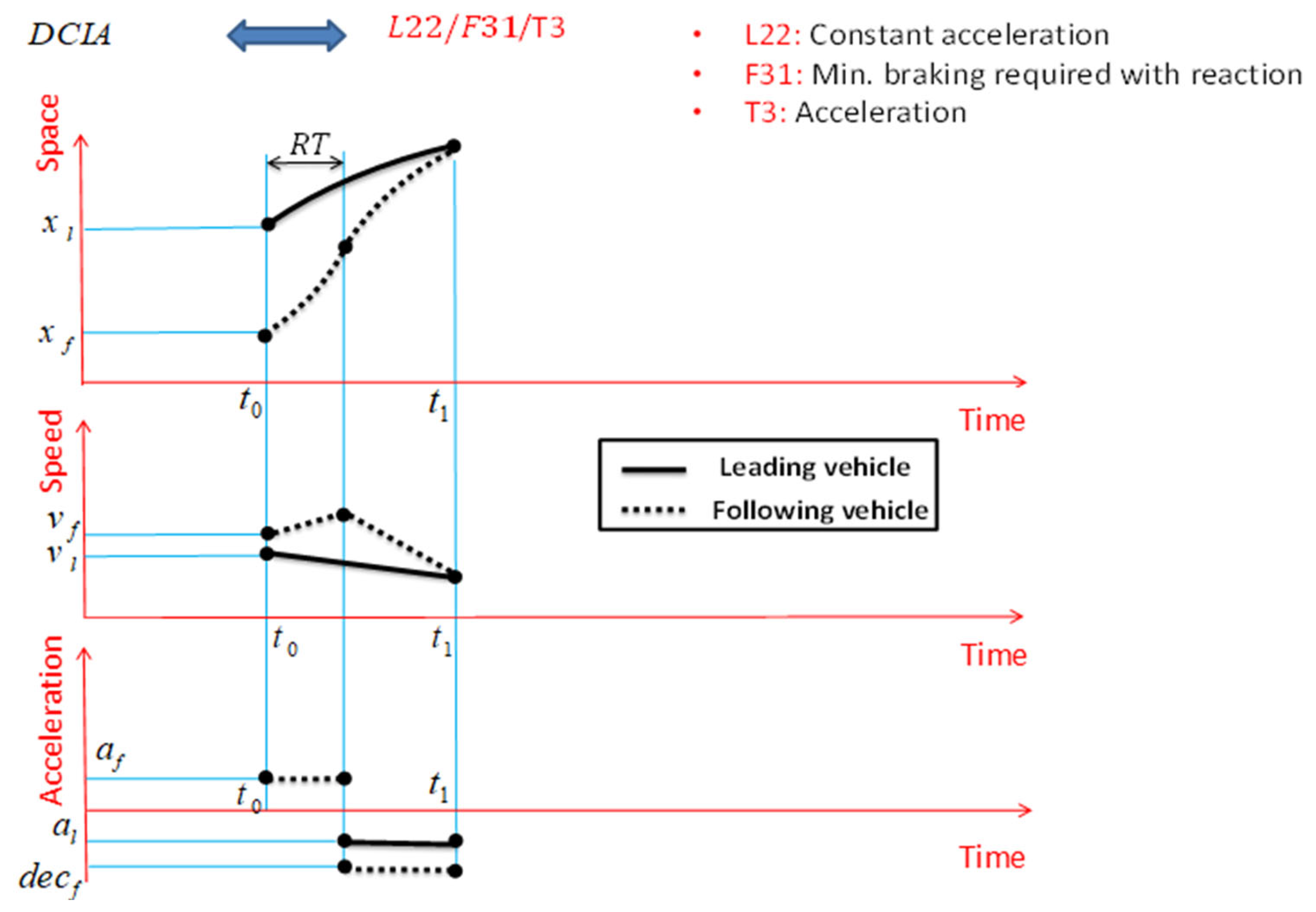
Fazekas et al. (2017) introduced a new SSM to describe risk called Deceleration to Avoid a Crash with Initial Acceleration (DCIA) by combining reaction time with a more realistic assumption about braking and acceleration behavior [24]. Unlike DRAC and MDRAC, DCIA is suitable for scenarios where the speed of the following vehicle is lower than the leading vehicle. Since DCIA does not assume constant speed profiles but has a constant acceleration, it can account for dangerous conditions where the following vehicle may have a lower speed but much higher acceleration than the leading vehicle. DCIA is obtained from Equation (9):

$$DCIA={\displaystyle \frac{a_{l}T+v_l-a_{f}R-v_f}{T-R}}$$

(9)

In this equation, $a_l$ and $v_l$ are the initial acceleration (which is constant) and speed of the leading vehicle, and $a_f$ and $v_f$ are the initial acceleration and initial speed of the following vehicle. Also, R is the reaction time, and T, which is the time when the speeds of the two vehicles reach a similar value, is obtained by the formula $T={\displaystyle \frac{v_{f}R-v_{l}R-2D}{v_l-a_{l}R-v_f+a_{f}R}}$, where D is the initial distance between the two vehicles.

3. Materials and Methods

In most Surrogate Safety Measures (SSMs), information about the instantaneous kinematic state of two consecutive vehicles, such as location, speed, and acceleration, is used to determine the safety status of those vehicles at the current time. For this purpose, the safety status of the following vehicle (i.e., the vehicle of interest) is assessed in a binary fashion: safe vs. unsafe. Also, in this regard, scenarios or storytelling of the near-future kinematic behavior of both the leading and following vehicles are presented. As shown in Figure 1, the storytelling for the vehicles is presented in a way that their kinematic conditions may become critical and ultimately lead to a collision.

Our proposed framework focuses on deconstructing the implicit assumptions within each SSM by mapping them to explicit, short-term motion scenarios. These scenarios or “stories” transparently articulate the foundational assumptions about how vehicles are expected to interact. To represent the relationship between these scenarios and the resulting SSM, we use a coding system inspired by the notational structure of queuing theory. It is important to clarify that this analogy is purely inspirational and notational; it does not import the mathematical or probabilistic dynamics of queuing systems. Its purpose is to provide a standardized, decomposable code for interaction scenarios by separating the story for the leading vehicle (L), the story for the following vehicle (F), and the type of indicator (T) with a “/” sign. Figure 1 represents a comprehensive classification of potential scenarios for the kinematic behavior of both the leading and following vehicles. For clarity and ease of reference, each scenario is identified with a unique code.

This figure illustrates the proposed framework for describing and categorizing the behavioral assumptions of SSMs through the concept of storytelling. Based on this framework, the kinematic behavior of each of the vehicles involved in the interaction (leading and following vehicles) in the short-term future after the current moment is considered as a story. These stories reflect the key assumptions of each SSM indicator about how vehicles interact and how their kinematic state changes on the verge of a hazard. The present figure provides a comprehensive set of possible stories for both vehicles. These stories categorize potential kinematic behaviors into three general levels:

• Leading vehicle (L):
  • L1: Motionless: The leading vehicle remains stationary without changing its speed or position.
  • L2: Continuous motion: The leading vehicle continues to move in one of the following three ways:
    • L21: Constant speed: The speed of the leading vehicle remains constant over time.
    • L22: Constant acceleration: The acceleration of the leading vehicle remains constant over time (maybe positive or negative).
    • L23: Constant jerk: The rate of change of acceleration (jerk) of the leading vehicle remains constant over time.
  • L3: Deceleration with max. braking: The leading vehicle reduces its speed with its maximum braking capacity.
• Following vehicle (F):
  • F1: Continuous motion: The following vehicle continues to move in one of the following three ways:
    • F11: Constant speed: The speed of the following vehicle remains constant over time.
    • F12: Constant acceleration: The acceleration of the following vehicle remains constant over time.
    • F13: Constant jerk: The rate of change of acceleration (jerk) of the following vehicle remains constant over time.
  • F2: Deceleration without reaction: The following vehicle starts to decelerate without considering the behavior of the leading vehicle and without time delay:
    • F21: Min. braking required: The following vehicle reduces its speed with the minimum braking required to avoid collision.
    • F22: Max. braking: The following vehicle reduces its speed with its maximum braking capacity.
  • F3: Deceleration with reaction: The following vehicle, after a time delay (driver reaction time) and in response to the behavior of the leading vehicle, starts to decelerate:
    • F31: Min. braking required: The following vehicle reduces its speed with the minimum braking force required to avoid collision.
    • F32: Max. braking: The following vehicle reduces its speed with its maximum braking capacity.

Each of these stories is identified by a unique code (such as L1, F22), which allows for easier reference and categorization. This figure shows how the behavioral assumptions of a particular SSM can be described precisely and systematically by combining a story for the leading vehicle and a story for the following vehicle. For example, the basic Time-To-Collision indicator (TTC1) is formed based on the story of constant speed movement for both vehicles (L21/F11).

This storytelling framework not only helps to understand the implicit assumptions of existing SSMs more deeply but also provides a platform for developing new SSMs by considering specific behavioral scenarios or aiming to cover the weaknesses of existing SSMs.

After defining the possible stories for the movement of each of the vehicles, the next step is to determine the type of SSM. As shown in Figure 2, SSMs can be divided based on their nature into four general categories:

• T1: Time-based
• T2: Distance-based
• T3: Acceleration-based
• T4: Ratio-based, which includes time ratio (T41), distance ratio (T42), and acceleration ratio (T43).

To represent the interaction and the SSM used, and the way the assumptions are storytelling for the movement of the two leading and following vehicles, we will use symbols similar to the pattern of what is used in queuing theory. In queuing theory, the characteristics of the input distribution and the output distribution, the number of service gates, and the queuing system are often separated by intervals so that a queuing system status can be represented. Here, we separate the storytelling for the movement of the leading vehicle, the storytelling for the movement of the following vehicle, and the type of SSM that can show the interaction of the two leading and following vehicles with intervals from each other. For instance, in the case of TTC1, we can represent it as L21/F11/T1 using a pre-defined coding system. This notation assumes that both the leading and following vehicles maintain a constant speed (kinematic state L21 and F11, respectively) and that TTC₁ is a time-based SSM (SSM, denoted by T1). Figure 3 presents assumptions regarding the motion status of the leading and following vehicles to define the classic Time-To-Collision or TTC1, along with the $x_t$, $v_t$, and graphs of the leading and following vehicles.

This figure presents assumptions about the kinematic state of the leading and following vehicles for defining and calculating the classical Time-to-Collision or TTC1, along with the $X_t$, $V_t$, and graphs of the leading and following vehicles. According to this figure, the goal is to calculate the value of the TTC1 indicator at time t₀, and for this purpose, it is assumed that both the leading and following vehicles are moving at a constant speed, and therefore their acceleration changes with time are equal to zero. The value of TTC1 is equal to the time from now, i.e., the current time t₀, until the two vehicles collide with each other. It should be explained that the reference points for drawing the path of the leading and following vehicles are the rear bumper of the leading vehicle and the front bumper of the following vehicle, respectively.

4. Results

Following the pattern of Figure 3, the motion assumptions of the leading and following vehicles for defining and calculating SSM, along with the x(t), v(t), and diagrams, have been drawn for the other SSMs presented in Table 2. This systematic application demonstrates how the framework not only categorizes existing measures but also reveals the evolutionary and hierarchical relationships between them. For example, the progression from DRAC to MDRAC is clarified as a specific change in the following vehicle’s assumed reaction (F21 to F31), while the core assumption about the lead vehicle (L21) remains constant. This structure provides a clear and addressable system for understanding, comparing, and ultimately selecting the most appropriate SSM for a given analysis context. Based on the concept of TTC2 and considering that the motion status of both the leading and following vehicles is assumed to have constant acceleration in this SSM, and considering that the type of SSM is time-based, TTC2 is represented with the coding defined in the Methodology section (based on the queuing theory structure) as L22/F12/T1. According to Figure 4 and assuming constant acceleration of the two vehicles in the car-following process, the speeds of the leading and following vehicles change at a constant rate over time. The value of TTC2 is equal to the time from now, i.e., the current time t₀, until the two vehicles collide with each other.

Given the assumptions made in defining TTC3, the motion status of both the leading and following vehicles in this SSM is with constant jerk, so considering that the type of SSM is time-based, TTC3 is shown as L23/F13/T1. Also, according to Figure 5 and assuming constant jerk of the two vehicles in the car-following process, the acceleration of the leading and following vehicles changes at a constant rate over time, and their speeds are increasing or decreasing at a variable rate until the moment of collision.

Based on the literature for TTCD and Figure 6, the assumption is that the leading vehicle brakes with the maximum possible rate, and the following vehicle continues to move at a constant speed. Therefore, considering that this SSM is also time-based, TTCD is displayed with the coding L3/F11/T1.

According to Figure 7, the assumption for DRAC is that the leading vehicle moves at a constant speed, and the following vehicle stops without reaction time with the minimum required braking. Therefore, considering that this SSM is acceleration-based, DRAC is displayed with the coding L21/F21/T3.

Regarding MDRAC and Figure 8, the assumptions are movement of the leading vehicle at a constant speed and braking of the following vehicle after reaction time and with the minimum required braking. Therefore, considering that this SSM, like DRAC, is acceleration-based, it will be shown with the coding L21/F31/T3.

In Figure 9 and PSD indicator, the assumption is that the leading vehicle, regardless of its speed and acceleration, is stationary at its position without motion. It is also assumed that the following vehicle stops without reaction time with the maximum required braking. Therefore, considering that this SSM is of the distance ratio type, it is displayed with the coding L1/F22/T42.

According to the concept of MPSD and the explanations in Figure 10, this SSM is of the distance-ratio type, and it is assumed that, like PSD, the leading vehicle, regardless of its speed and acceleration, is stationary at its position without motion, and the following vehicle brakes at the maximum possible rate after reaction time. Therefore, this SSM is shown as L1/F32/T42.

According to the assumptions made in the literature, DCIA is acceleration-based, and the motion status of the leading vehicle is with constant acceleration. Also, the following vehicle performs braking after reaction time and at the minimum required braking. Therefore, DCIA is displayed with the code L22/F31/T3. Also, according to Figure 11 and assuming constant acceleration of the two vehicles in the car-following process, the speeds of the leading and following vehicles change at a constant rate, increasing and decreasing over two time periods.

Finally, the coding method of SDI is as follows. This SSM is distance-based. According to Figure 12, it is assumed that the leading vehicle brakes at the maximum braking rate, and the following vehicle brakes with the maximum possible rate after reaction time. Therefore, the SDI is shown as L3/F32/T2.

At the end of this section, all SSMs studied are summarized in

Table 4. Naming of some SSMs in the presented framework.

		Assumptions for Following Vehicle Motion
		F11	F12	F13	F21	F22	F31	F32
Assumptions for Leading Vehicle motion	L1	THDW				PSD		MPSD
	L21	TTC1			DRAC		MDRAC
	L22		TTC2				DCIA
	L23			TTC3
	L3	TTCD						SDI

according to the defined framework based on the concept of each SSM and queuing theory pattern in a systematic way. In some of the cells of the table that are empty, it will be possible for researchers to develop new SSMs in the future by defining the storytelling of the movement of the leading and following vehicles.

5. Discussion

This research introduces a conceptual framework, termed Motion Scenario Mapping, to systematically categorize and understand Surrogate Safety Measures (SSMs) used in traffic safety analysis. By employing a storytelling approach rooted in queuing theory, the framework elucidates the implicit assumptions underlying each SSM, offering a more nuanced understanding of their applicability and limitations. The analysis of ten widely used SSMs demonstrates the framework’s effectiveness in revealing these hidden assumptions, thereby facilitating more informed selection and application of these measures. The true value of this research lies not merely in cataloging existing measures but in providing a structured foundation for future research, development, and application within an increasingly complex transportation landscape.

A critical direction for future work involves empirical validation of the framework’s utility. Although this paper establishes the conceptual foundation, its practical advantages in improving safety analysis require quantitative demonstration. A clear validation pathway involves utilizing large-scale, high-resolution vehicle trajectory data, such as datasets from NGSIM, highD, or connected vehicle streams. One proposed validation study could involve scenario-based SSM evaluation by identifying specific traffic conflict scenarios, such as hard braking or cut-ins, and selecting candidate SSMs whose “stories” best align with observed dynamics. Performance comparison would correlate the outputs of these SSMs with actual conflict outcomes, hypothesizing that SSMs with stories closely matching real-world kinematics will exhibit stronger risk correlation. Furthermore, this approach can enhance interpretability by clearly explaining why certain SSMs perform better or worse, effectively demonstrating the framework as more than just a classification tool, but rather a diagnostic aid for more accurate and reliable safety assessments.

The rise of intelligent and autonomous vehicles (AVs), particularly in mixed traffic scenarios, underscores the necessity for a granular understanding of interaction dynamics. The storytelling framework provides powerful implications for AV development and safety assurance. For instance, an AV’s control system can employ the framework to classify the real-time behavior of an interacting vehicle—identifying it as L21 (constant speed) or L22 (constant acceleration)—and subsequently select an optimal counter-maneuver from its behavioral library, such as a reactive braking profile (F31). Furthermore, the framework offers a structured methodology for systematic safety validation, enabling developers to generate comprehensive test suites covering all plausible interaction stories, such as verifying an AV’s response to an L3/F11 scenario where a lead vehicle brakes maximally. Moreover, it helps address human–AV interaction challenges, which often arise from mismatched expectations. Engineers can use the framework to explicitly compare an AV’s programmed story, perhaps an efficiency-focused F12, with the reactive F31 story a human driver might anticipate, thereby aiding in the design of AVs perceived as both predictable and trustworthy.

The L/F/T notation is a foundational model designed for scalability. It can be extended to accommodate more complex scenarios, such as multi-vehicle interactions (L/F1/F2/T) or conflicts with vulnerable road users by introducing new actor types (P for pedestrians). Furthermore, the framework’s deterministic assumptions can be extended. To capture the evolution of risk over time, the “story” classifications could be integrated into time-to-event or hazard function models. To account for real-world uncertainty, a probabilistic layer could be added, for instance, by extending the notation (/S for stochastic) or by using the deterministic stories as mean functions within Bayesian models to account for sensor noise and driver variability.

Finally, it is important to position this framework alongside modern AI-based and theory-driven approaches. Recent advances in safety analysis leverage spatio-temporal prediction, traffic flow theory, and deep learning models (e.g., LSTMs) to forecast trajectories and risk. Our framework is not a competitor to these sophisticated models but a complementary, foundational tool. It provides a structured, qualitative understanding of the underlying risk primitives (the “stories”) that can inform feature engineering, scenario generation for training data, and the interpretability of “black-box” AI models, thereby bridging the gap between advanced quantitative methods and intuitive, assumption-aware safety assessment.

6. Conclusions

Selecting an appropriate surrogate safety measure (SSM) has always been a challenge, given the variety and sometimes conflicting viewpoints of researchers. Therefore, this research aimed to create a systematic framework, Motion Scenario Mapping, for examining and analyzing the safety status of vehicles in the car-following process.

To achieve this, we presented a novel framework based on the concept of storytelling the motion assumptions of vehicles in the near future. We reviewed 10 widely used and accepted SSMs from the literature and analyzed their functionality. The framework utilizes innovative coding based on queuing theory and draws diagrams of changes in location, speed, and acceleration over time (x(t), v(t), and a(t)) to provide a comprehensive and systematic view for understanding and categorizing existing SSMs.

The final table resulting from this study provides a practical tool for informed selection of SSMs based on various motion scenarios of leading and following vehicles. Furthermore, the presented structure provides a basis for developing new SSMs by considering diverse combinations of motion behaviors that have received less attention so far. This coding allows for the definition of similar SSMs by new researchers in the future, addressing components of vehicle motion previously overlooked. Gradually filling the empty cells of the table with new SSMs will ensure the dynamism and comprehensiveness of this framework. As a direction for future research, this framework lays out a clear and structured agenda. The most critical next step is the empirical validation of the framework using real-world trajectory data to demonstrate its utility in improving SSM selection and risk assessment. Furthermore, the empty cells in the classification matrix (Table 3) represent clear opportunities for innovation. Researchers are encouraged to develop new SSMs to fill these gaps, such as those modeling constant jerk interactions or new reactive behaviors relevant to autonomous systems. The framework itself can be extended to handle more complex scenarios, including multi-vehicle conflicts, interactions with vulnerable road users, and stochastic driver behaviors. Finally, applying this framework to the design and verification of autonomous vehicle control logic can help ensure that AVs operate safely and predictably in mixed-traffic environments. By providing a common language for interaction stories, this work aims to catalyze more harmonized, targeted, and impactful research in the ongoing quest for safer future transportation.