Visualizing Railway Transfer Penalties and Their Effects on Population Distribution in the Tokyo Metropolitan Area

Abstract

This study investigates the impact of railway transfer penalties on the demographic structure of the Tokyo Metropolitan Area. While previous research has emphasized travel time to the city center as a key determinant of socio-demographic structure, this paper highlights the additional influence of transfer penalties—specifically walking and waiting times—on urban demographic patterns. Using 1 km grids as the unit of analysis, travel time to Tokyo Station is calculated as a measure of accessibility, and the difference in travel time with and without accounting for transfers is defined as the transfer penalty for each grid. The spatial distribution of these penalties is mapped, and their effects on the population are estimated while considering heterogeneity based on distance to the city center. The results indicate that beyond accessibility, higher transfer penalties are associated with lower population densities. Moreover, the negative impact of transfer penalties is observed only in areas located at an intermediate distance from the city center (approximately 26–46 km). Finally, incorporating this spatial heterogeneity, the paper visualizes the projected contribution of transfer penalties to future population distribution.

1. Introduction

The convenience of public transportation in urban areas can significantly influence the socio-demographic structure by shaping patterns of residential and industrial activity. In particular, rail accessibility—commonly assessed through station proximity and travel time to the city center—can enhance a city’s attractiveness and spur development. However, it may also contribute to socio-spatial disparities.

For example, improved accessibility can drive gentrification, whereby the influx of middle- to high-income residents leads to rising housing prices and a decline in affordability for low-income populations, ultimately undermining their residential stability and overall livability [1]. This phenomenon, known as transit-induced gentrification, occurs when new public transportation is introduced in areas where low-income households are concentrated. The resulting increase in convenience and associated redevelopment attracts middle- and high-income residents while displacing lower-income populations due to rising living costs. From this perspective, while transportation development enhances the overall attractiveness of urban areas, it can also exacerbate inequalities in access.

Recent studies have leveraged theoretical advances in spatial economics and the growing availability of geospatial data, such as satellite imagery and GIS tools, to empirically examine the impacts of transport network development on socio-economic situations [2,3]. These studies suggest that although railway development contributes to national economic growth, its benefits are often concentrated in major urban centers [4]. Further research has found that improvements in accessibility—such as reduced distance to stations and the introduction of new railway lines—are associated with increased local income levels and higher rates of college graduation [5,6,7]. Thus, the socio-economic impacts of rail accessibility, especially regarding station proximity and travel time to city centers, have been well documented.

However, accessibility is not the only aspect of transportation development that may influence socio-demographic structures. One underexplored factor is transfer convenience. Transfer-related burdens—including walking time, waiting time, and general inconvenience—are known to create disutility for travelers [8]. In this sense, areas with direct routes to city centers and fewer required transfers may be perceived as more attractive. If transfer convenience increases the residential appeal for middle- and high-income earners, a concentration of population in such areas could contribute to further socio-economic stratification. While the relationship between accessibility and socio-demographic outcomes is well established, the role of transfer convenience remains insufficiently understood.

Furthermore, the inconvenience of transferring may contribute to the widening of additional disparities apart from accessibility. It has been found that transportation disadvantage can lead to social exclusion and segregation, contributing to disparities in access to employment, urban services, education, and healthcare for low-income groups [9,10,11]. In this context, not only overall accessibility but also the inconvenience of transferring between transport routes may further exacerbate spatial inequalities by limiting individuals’ ability to participate fully in various activities.

In transportation research, the concept of the transfer penalty has gained attention as an important complement to traditional measures such as station proximity and travel time. The transfer penalty refers to the perceived disutility associated with transferring trains, including waiting time, walking time, and the inconvenience of making the transfer itself [8]. Previous studies have shown that transfer penalties are perceived by users as a source of inconvenience, unreliability, and wasted time [12]. Based on this understanding, it is plausible that areas with high transfer penalties may experience reduced attractiveness and lower residential demand. Nevertheless, the extent to which transfer penalties influence spatial demographic patterns remains unclear.

This paper examines the effect of train transfer penalties on population distribution in the Tokyo Metropolitan Area as of 2020 while controlling for rail accessibility. The Tokyo region is characterized by an extensive rail network, with approximately 40 operators managing over 100 train lines, making transfers a common part of daily travel. This study calculates transfer penalties—incorporating both walking and waiting times—using 1 km mesh units that cover the entire metropolitan area. Moreover, since transfer penalties may have less impact when total travel time is already short, the analysis includes a subsample approach to explore how these effects vary by distance from the city center.

The main contribution of this paper is to clarify the influence of transfer penalties on population distribution while accounting for spatial heterogeneity based on proximity to the urban core. By analyzing these dynamics, this study provides insight into how transfer-related disutility contributes to the socio-demographic structure of cities and identifies the specific distance range from the city center where such effects are most pronounced.

2. Materials and Methods

2.1. Data

In this study, I used data from the Digital National Land Information (DNLI) provided by the Ministry of Land, Infrastructure, Transport and Tourism of Japan for our analysis (https://nlftp.mlit.go.jp/ksj/, accessed on 14 March 2025). The unit of analysis was a 1 km × 1 km area mesh, which divided the entire land surface of Japan into standardized grid cells, each identified by a unique mesh code. For the purposes of network analysis, I used the geometric center of each mesh as the origin point.

The dependent variable in this study is the population at the mesh level, using both current and projected data. The DNLI provides population figures for the year 2020, as well as future population projections. These projections are available in 10-year increments from 2030 to 2070.

To evaluate rail accessibility and transfer penalties, I used railway line data and station point data obtained from the DNLI. Using ArcGIS Pro, I constructed a network dataset based on the obtained GIS data. I designated Tokyo Station as the destination point, which enables us to calculate travel times and transfer penalties from each mesh to Tokyo Station via rail.

2.2. Study Area

This study focuses on the Tokyo Metropolitan Area in 2020, the largest metropolitan region in Japan and one that is highly dependent on rail transportation. In particular, within the 23 special wards of Tokyo—the city’s central core—railways account for approximately 50% of all trips [13]. Given this high reliance on rail transport, the influence of railway accessibility and transfer penalties on daily mobility is substantial, making the Tokyo Metropolitan Area a suitable case for analysis. In addition, compared to major cities worldwide, Tokyo’s 23 wards have the second-highest station and rail line density after Paris, surpassing cities such as New York, Seoul, London, and Singapore [14]. In cities with such high railway density, rail usage is typically high; however, transfer penalties are likely to have a particularly significant impact on travel behavior.

There are multiple definitions of the Tokyo Metropolitan Area; in this study, I adopted the Urban Employment Area definition proposed by [15]. Unlike administrative boundaries, this definition is based on functional linkages shaped by socio-economic activity. Specifically, it defines a metropolitan area as comprising a central city—identified by densely inhabited districts (DIDs)—and surrounding municipalities with a commuting rate of 10% or higher to the central city.

In this study, I used the Tokyo Metropolitan Employment Area as the spatial scope of analysis. I used the list of cities included in the Tokyo Metropolitan Employment Area as defined by [16] to determine the spatial boundaries of the study area. Figure 1 presents the study area, including railway lines and population distribution at the 1 km grid level. Tokyo Station is designated as the destination point for calculating accessibility and transfer penalties. Located in the Marunouchi district—Tokyo’s business center—Tokyo Station is widely recognized as a major transportation hub in the metropolitan region [17].

To focus the analysis on accessibility from suburban and sub-center areas to the city’s core, I excluded Chiyoda Ward, Minato Ward, and Chuo Ward—three wards located in the city center—from the analysis. The remaining area encompasses approximately 130 railway lines operated by 40 different railway companies.

2.3. Variables and Estimation Model

Mesh-level accessibility and transfer penalties were calculated using a network dataset comprising mesh center points, railway stations, railway lines, and Tokyo Station. The origin of each trip was defined as the center point of each mesh, with Tokyo Station set as the destination. Travel time to Tokyo Station via the railway network was calculated and used as a measure of accessibility for each mesh.

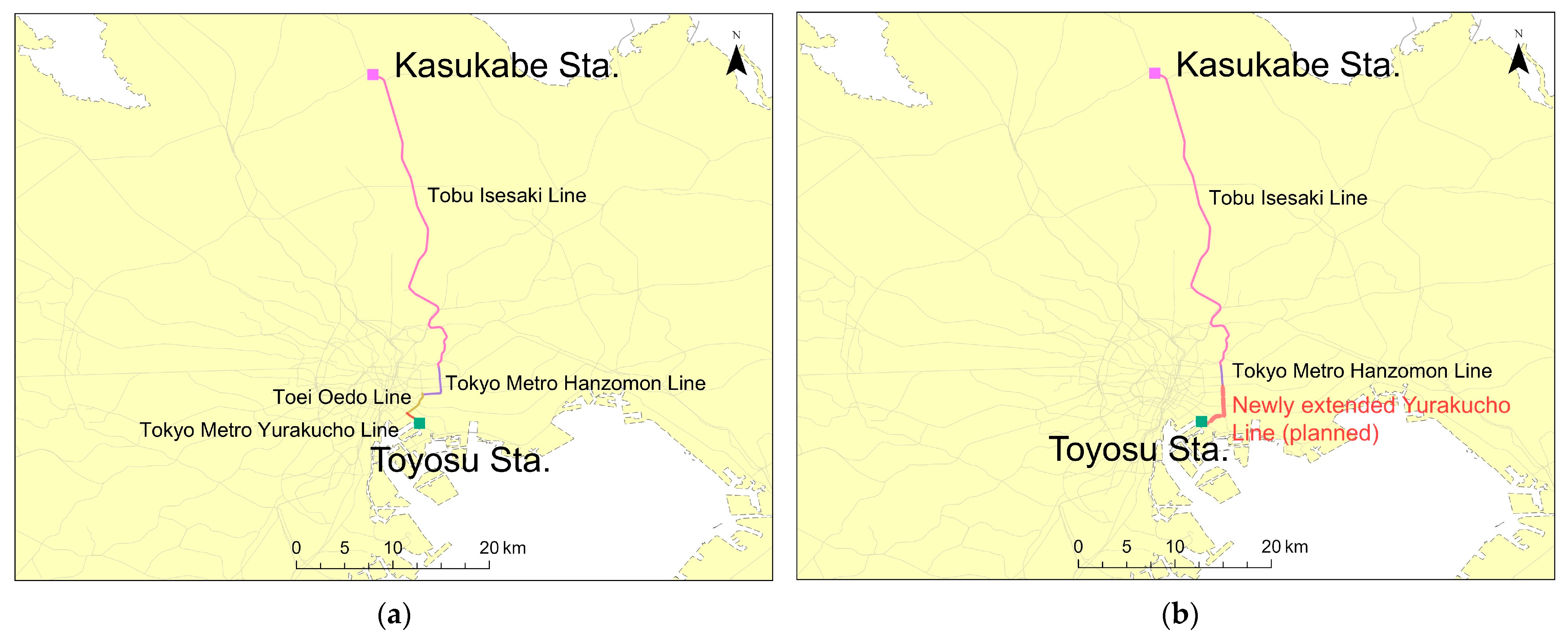
To quantify the transfer penalty, the waiting time corresponding to each railway station was predicted based on the train frequency data. The transfer penalty for a mesh was then defined as the difference in travel time to Tokyo Station with and without this transfer-related waiting time. Figure 2 illustrates the conceptual framework used for calculating travel time and transfer penalties.

The specific method for calculating mesh-level accessibility and transfer penalties was explained using the notation presented in Figure 2. As the index of accessibility, the travel time from grid o to Tokyo Station without transfer penalty was calculated as follows:

$$t_{o, nopen}=t_{wait,s,0}+{\displaystyle \frac{d_o}{v_{walk}}}+\sum _l{\displaystyle \frac{d_{li}}{v_{rail}}}+\sum _k{\displaystyle \frac{d_{trf,k}}{v_{walk}}}+{\displaystyle \frac{d_d}{v_{walk}}},$$

(1)

where $t_{wait, s,0}$ refers to the waiting time for the first train station $s_0$, $d_o$ is the Euclidean distance from the center of grid o to the first railway station on a route, $d_{li}$ is the length of the rail line $l_i$ from the origin station to the destination station, $d_{trf,k}$ is the walking distance for transfers for the transfer ${trf}_k$ (kth transfer), and $d_d$ is the distance from the destination station to Tokyo Station. If transfers are possible at the same station, $d_{trf,k}$ becomes zero. If it is possible to reach Tokyo Station directly by railway, $d_d$ becomes zero. $v_{walk}$ and $v_{rail}$ are the assumed speeds for walking and railway, respectively. In addition, if the travel distance to the first station $d_o$ exceeds 1 km, it is assumed that the distance beyond 1 km will be traveled by other means of transportation (e.g., bus, car, motorcycle, etc.) since it is not realistic to travel such a long distance on foot. In this case, the travel speed for the additional distance is set to 30 km/h.

In addition, the travel time with a transfer penalty was assumed to be as follows:

$$t_{o, pen}=t_{wait, s,0}+{\displaystyle \frac{d_o}{v_{walk}}}+\sum _l{\displaystyle \frac{d_{li}}{v_{rail}}}+\sum _k\left({\displaystyle \frac{d_{trf,k}}{v_{walk}}}+t_{wait, s,k}\right)+{\displaystyle \frac{d_d}{v_{walk}}},$$

(2)

where $t_{wait, s,k}$ is the waiting time for the next train for a transfer ${trf}_k$ at station $s_k$. This means that for the kth transfer at the station $s_k$, it will take $t_{wait,s,k}$ for the next train. In this analysis, I assumed that $v_{walk}$ is 4 km/h and $v_{rail}$ is 80 km/h, respectively, based on previous studies [18]. For this analysis, travel times are calculated in minutes.

In addition, I predicted $t_{wait,s}$ based on the data of the frequency of trains for each railway station obtained from [19]. Train intervals are inversely proportional to train frequency. Assuming that passenger arrivals at stations are random, the average waiting time for a train is half the interval between trains. Consequently, the average waiting time is also inversely proportional to train frequency. Based on this logic, the average waiting time at each station was calculated using the following formula:

$$t_{wait,s}={\displaystyle \frac{a}{{frequency}_s}},$$

(3)

where $t_{wait,s}$ represents the average waiting time at station s, and ${frequency}_s$ denotes the train frequency at station s. The constant a is predicted using observed data from example stations. I selected Sasazuka Station, which has the highest train frequency in the dataset, and Shimo-Itabashi Station, which has the median frequency among stations in the target area. Sasazuka Station operates up to 387 trains per day, corresponding to an average waiting time of approximately 2 min during rush hours. Shimo-Itabashi Station operates up to 157 trains per day, with an average waiting time of about 5 min during rush hours. Based on these values, I set a = 779 for calculating waiting times across all stations. As a result, the median estimated waiting time was 4.96 min, and the minimum was 2.01 min.

To calculate the shortest routes, I used ArcGIS Pro to perform a network analysis. The network was constructed using the centers of each mesh, all railway stations, and Tokyo Station (the final destination) as nodes, with railway lines serving as edges. Additionally, several necessary supplementary edges were added: (1) Mesh-to-station connections—edges were created between the center of each mesh and all railway stations within a 5 km radius, representing access from the mesh to nearby railway stations. (2) Final destination connections—edges were created between all railway stations within 1 km of Tokyo Station, representing the final walking segment from a nearby station to Tokyo Station itself. (3) Transfer connections—edges were created between all railway stations located within 1 km of each other to account for transfers between closely situated stations.

Using this network, I determined the shortest route from each mesh to Tokyo Station. Travel time, as defined in Equations (1) and (2), was used as the cost function for route selection. The shortest travel time computed using Equation (1), which does not account for transfer waiting times, was denoted as ${\tau }_{o, nopen}$. On the other hand, the shortest travel time using Equation (2), which assumes a waiting time for each transfer, was denoted as ${\tau }_{o, pen}$. The transfer penalty was then calculated as follows:

$${penalty}_o={\tau }_{o, pen} - {\tau }_{o, nopen}$$

(4)

It is important to note that the shortest route without transfer waiting time and the shortest route with transfer waiting time are not necessarily the same. Under the assumption of Equation (2), an additional waiting time was added for each transfer compared to Equation (1). For example, consider two routes: Route A requires one transfer and takes 20 min without considering transfer waiting time, and Route B does not require any transfer and takes 25 min. If transfer waiting time is not considered, Route A is the shortest, and ${\tau }_{o, nopen}=20$. However, if each transfer adds a 10 min penalty, the travel time for Route A becomes 30 min, making Route B the shortest, and ${\tau }_{o, pen}=25$. In this case, the transfer penalty is ${\tau }_{o, pen} - {\tau }_{o, nopen}=25 - 20=5 \mathrm{m}\mathrm{i}\mathrm{n}$.

The impact of the absolute value of penalty time depends on the length of the original travel time. Therefore, in addition to the penalty in minutes, I calculated the rate of the increase in travel time due to the transfer as follows:

$${penalty\_ratio}_o={\displaystyle \frac{{\tau }_{o, pen} - {\tau }_{o, nopen}}{{\tau }_{o, nopen}}}.$$

(5)

Using the indices calculated above, I estimated the following OLS model to clarify the impact of accessibility and transfer penalties on current and future population distribution:

$$\ln \left({pop}_o\right)={\beta }_0+{\beta }_1\ln \left({\tau }_{o, nopen}\right)+{\beta }_2\ln \left({penalty}_o\right)+{graduate}_o+{\delta }_r+{\epsilon }_o,$$

(6)

where ${pop}_o$ is the number of populations living in mesh o, and ${\delta }_r$ is a city fixed effect. In Equation (6), ${\beta }_1$ and ${\beta }_2$ represent the effects of a 1% increase in travel time to Tokyo Station and a 1% increase in transfer penalty on the number of passengers, respectively. ${graduate}_o$ represents the university graduation rate for the town in which mesh o is located. This variable is included to control for the socio-demographic characteristics of the area, in place of income level, which is not available at the fine spatial resolution. Data on university graduation rates for the year 2020 were obtained from the Population Census of Japan (https://www.e-stat.go.jp/statistics/00200521, accessed on 14 March 2025).

I also estimated the following model:

$$\ln \left({pop}_o\right)={\beta }_0+{\beta }_1\ln \left({\tau }_{o, nopen}\right)+{\beta }_2{penalty\_ratio}_o+{graduate}_o+{\delta }_r+{\epsilon }_o.$$

(7)

Compared to Equation (6), Equation (7) aims at estimating the effects of the ratio of transfer penalty to travel time on the population distribution. Additionally, to examine the impact on future population distribution, I also estimated a model that uses the projected population for 2030 and 2070 as supplementary dependent variables in addition to the current population (2020). Across all specifications, standard errors were clustered at the city level.

Table 1. Summary statistics (N = 6237).

Variable	Mean	Std. Dev.	Min	Max
${\tau }_{o, nopen}$ (min)	59.109	20.721	11.260	162.161
penalty (min)	6.016	6.408	0	61.458
penalty_ratio	0.101	0.072	0	0.524
university graduate rate	0.195	0.090	0	0.525
population 2020	5537.017	6120.472	81.695	32,601.270
population 2030 (projected)	5548.832	6291.164	29.178	34,481.940
population 2070 (projected)	4850.120	6029.268	0	35,916.250

shows the summary statistics of the variables.

3. Results

This section presents visualizations of accessibility and transfer penalties from each grid point to Tokyo Station, along with estimation results on how these variables affect current and future population distribution.

3.1. Visualizing Transfer Penalty

Figure 3 presents the calculated travel times from each grid to Tokyo Station, excluding transfer penalties. As expected, travel time increases with distance from the city center. However, the areas located along railway lines tend to exhibit relatively shorter travel times compared to the surrounding regions.

Figure 4 shows the calculated transfer penalty for each grid. While overall accessibility to the city center exhibits a roughly circular pattern, the distribution of transfer penalties is more radial, following the railway network. Even in areas located more than 50 km from Tokyo Station, transfer penalties are minimal or nonexistent when travel is possible via a single train line. In contrast, even within 10–20 km of the city center, transfer penalties of approximately up to 8 min begin to emerge. In some areas, penalties reach up to about 60 min, indicating that proximity alone does not guarantee high accessibility when transfers are involved.

3.2. The Impact of Transfer Penalty on Population Distribution

Table 2. Estimation results. Dependent variable: population 2020. Standard errors are reported in parentheses.

	(1)	(2)	(3)
$\ln \left({\tau }_{o, nopen}\right)$	−1.191 ***	−1.212 ***	−1.273 ***
	(0.118)	(0.121)	(0.137)
$\ln \left({penalty}_o\right)$		−0.0719 ***
		(0.026)
${penalty\_ratio}_o$			−0.510 **
			(0.227)
${graduate}_o$	2.095 ***	2.072 ***	2.071 ***
	(0.171)	(0.168)	(0.170)
Constant	13.07 ***	13.26 ***	13.44 ***
	(0.441)	(0.472)	(0.530)
N	6232	6232	6232
R-sq	0.671	0.672	0.672

*** p < 0.01, and ** p < 0.05.

presents the estimation results for the models specified in Equations (6) and (7). Specification (1) includes only travel time as the explanatory variable, serving as the baseline accessibility measure. Specifications (2) and (3) extend the model by including the transfer penalty in minutes and the transfer penalty ratio, respectively. The dependent variable in all cases is the population at the 1 km grid level in 2020.

In specification (1), a 1% increase in travel time is associated with approximately a 1.2% decrease in population. This relationship remains consistent across specifications, with only slight variations in magnitude. Specification (2) indicates that a 1% increase in the transfer penalty (in minutes) corresponds to an approximate 0.07% decrease in population. Specification (3) further reveals that a 1% increase in the ratio of transfer penalty to total travel time is associated with a 0.51% decrease in population.

These results suggest that even when general accessibility is accounted for, transfer penalties exert an additional negative effect on residential population distribution.

To demonstrate the appropriateness of applying logarithmic transformations to the dependent and explanatory variables, I compared the residual plots and AIC and BIC values from specification (2) with those from a model in which neither the dependent variable (2020 population) nor the independent variables (${\tau }_{o, nopen}$, ${penalty}_o$) are log-transformed. Figure 5 presents the residual plots for both models: Figure 5a corresponds to the model with log-transformed variables, while Figure 5b corresponds to the model without log transformations. The residuals in Figure 5b partially show a linear pattern, suggesting model misspecification, whereas the residuals in Figure 5a are more evenly dispersed, indicating a better model fit.

Table 3. Values of AIC and BIC for each specification.

	AIC	BIC
logY-logX	8163.319	8183.531
Y-X	119,288.8	119,309

reports the AIC and BIC values for both models. Both criteria are lower for the log-log model, further supporting its superior fit. These diagnostics suggest that applying logarithmic transformations improves the accuracy and specification of the model.

To explore whether the effect of transfer penalties varies by distance to Tokyo Station, I divided the mesh data into four equal groups based on their distance from Tokyo Station. For each subgroup, I conducted regression analyses similar to those presented in Table 2.

Table 4. Characteristics of subsamples divided by the distance to Tokyo Station.

Graph	Average Distance to Tokyo Station (km)	Range (km)	Average Time to Tokyo Station (min)	Range (min)
1	17.27	2.73–26.16	35.19	11.26–53.56
2	31.85	26.16–36.73	53.42	32.21–97.34
3	41.12	36.73–45.98	66.83	41.60–136.65
4	54.64	45.98–79.93	81.00	51.28–162.16

reports the average and range of both the distance to Tokyo Station and the corresponding travel time (${\tau }_{o, nopen}$).

Table 5. Estimation results for subsamples divided by the distance to Tokyo Station. Standard errors are reported in parentheses.

	Group 1		Group 2		Group 3		Group 4
	(2)	(3)	(2)	(3)	(2)	(3)	(2)	(3)
$\ln \left({\tau }_{o, nopen}\right)$	−0.752 ***	−0.758 ***	−2.061 ***	−2.160 ***	−3.434 ***	−3.488 ***	−3.333 ***	−3.414 ***
	(0.102)	(0.123)	(0.178)	(0.191)	(0.185)	(0.197)	(0.475)	(0.433)
$\ln \left({penalty}_o\right)$	−0.0321		−0.136 ***		−0.109 **		−0.0368
	(0.037)		(0.034)		(0.047)		(0.107)
${penalty\_ratio}_o$		−0.0859		−1.130 **		−1.312 *		0.937
		(0.252)		(0.448)		(0.767)		(1.558)
${graduate}_o$	1.407 ***	1.405 ***	1.966 ***	1.983 ***	2.462 ***	2.483 ***	2.917 ***	2.858 ***
	(0.231)	(0.234)	(0.271)	(0.270)	(0.508)	(0.506)	(0.745)	(0.723)
Constant	11.84 ***	11.83 ***	16.75 ***	17.02 ***	22.28 ***	22.43 ***	21.93 ***	22.20 ***
	(0.397)	(0.461)	(0.709)	(0.768)	(0.821)	(0.877)	(2.071)	(1.909)
N	1557	1557	1556	1556	1555	1555	1556	1556
R-sq	0.552	0.551	0.513	0.511	0.538	0.539	0.586	0.586

*** p < 0.01, ** p < 0.05, and * p < 0.1.

presents the estimation results by subsample. The coefficient for travel time is significantly negative across all the distance groups, indicating that longer travel times are consistently associated with lower population levels. In contrast, the transfer penalty exhibits a significantly negative effect only in Groups 2 and 3—those located at moderate distances from Tokyo Station. No significant effect is observed in Group 1 (closest to Tokyo Station) or Group 4 (farthest). These results suggest that transfer penalties influence population distribution primarily in areas that are neither too close nor too far from the urban core.

3.3. Transfer Penalty and Future Population Distribution

To examine the impact of transfer penalties on future population distribution, I conducted regression analyses using projected population data for 2030 and 2070 as the dependent variables.

Table 6. Estimation results. Dependent variable: future population. Standard errors are reported in parentheses.

	Population 2030	Population 2070
$\ln \left({\tau }_{o, nopen}\right)$	−1.313 ***	−1.355 ***
	(0.143)	(0.162)
${penalty\_ratio}_o$	−0.539 **	−0.597 **
	(0.234)	(0.251)
${graduate}_o$	2.218 ***	2.590 ***
	(0.175)	(0.186)
Constant	13.55 ***	13.47 ***
	(0.554)	(0.623)
N	6232	6232
R-sq	0.681	0.719

*** p < 0.01, and ** p < 0.05.

presents the estimation results using projected population values for 2030 and 2070 as dependent variables. In both cases, travel time to Tokyo Station has a consistently negative effect on the population. Similarly, the transfer penalty ratio also shows a negative association with future population distribution, consistent with the findings for the 2020 population. These results suggest that even when overall accessibility is held constant, the grids with higher transfer penalties are expected to experience lower future population levels. Moreover, the magnitude of the coefficient is larger for 2070 than for 2030, indicating that the negative impact of transfer penalties may become more pronounced over time.

Table 7. Estimation results for subsamples. Dependent variable: future population. Standard errors are reported in parentheses.

	Group 1		Group 2		Group 3		Group 4
Projection Year	2030	2070	2030	2070	2030	2070	2030	2070
$\ln \left({\tau }_{o, nopen}\right)$	−0.768 ***	−0.717 ***	−2.261 ***	−2.439 ***	−3.640 ***	−4.030 ***	−3.497 ***	−3.786 ***
	(0.126)	(0.126)	(0.195)	(0.215)	(0.195)	(0.217)	(0.448)	(0.527)
${penalty\_ratio}_o$	−0.0971	−0.0736	−1.156 **	−1.232 **	−1.464 *	−2.076 **	1.014	1.15
	(0.258)	(0.260)	(0.461)	(0.478)	(0.783)	(0.852)	(1.591)	(1.705)
${graduate}_o$	1.554 ***	1.903 ***	2.108 ***	2.435 ***	2.605 ***	2.912 ***	2.950 ***	3.208 ***
	(0.244)	(0.262)	(0.275)	(0.287)	(0.505)	(0.528)	(0.745)	(0.825)
Constant	11.85 ***	11.51 ***	17.38 ***	17.80 ***	23.01 ***	24.30 ***	22.48 ***	23.24 ***
	(0.470)	(0.473)	(0.784)	(0.858)	(0.867)	(0.947)	(1.976)	(2.325)
N	1557	1557	1556	1556	1555	1555	1556	1556
R-sq	0.557	0.586	0.517	0.539	0.543	0.565	0.59	0.617

*** p < 0.01, ** p < 0.05, and * p < 0.1.

presents the estimation results for subsamples divided by the distance to the Tokyo Station. Consistent with the findings in Table 5, transfer penalties have a significantly negative effect on future population in Groups 2 and 3. Moreover, the absolute value of the coefficient is slightly larger when using the 2070 population as the dependent variable compared to 2030, suggesting that the influence of transfer penalties may intensify over time.

I also visualized the impact of transfer penalties on future population distribution. The contribution of transfer penalties to population change was calculated using the following formula:

$$\%\Delta {pop}_{ot}={\widehat{\beta }}_{2t}{penalty\_ratio}_o\times 100,$$

(8)

where $\%\Delta {pop}_{ot}$ represents the percentage change in population in grid o in year t (2030 or 2070), attributable to transfer penalties compared to a scenario without transfer-related waiting time. The estimated coefficients ${\widehat{\beta }}_{2t}$ are drawn from the regression results in Table 7, and differ by distance-based group, reflecting the heterogeneous effects of transfer penalties depending on proximity to Tokyo Station.

Figure 6 visualizes these results. Darker blue areas indicate a stronger negative impact of transfer penalties on population. The figure shows that in Groups 2 and 3—corresponding to meshes located 26.16 to 45.98 km from Tokyo Station—some areas experience a substantial population decline due to transfer penalties. However, within the same distance range, areas with fewer required transfers show less impact. In contrast, for Group 4 (meshes located more than 45.98 km from Tokyo Station), the effect of transfer penalties on population decline is minimal or negligible.

These results indicate that transfer penalties do not uniformly affect all suburban areas. Instead, their impact is concentrated in intermediate-distance zones, suggesting that addressing transfer inefficiencies in these regions may be more effective than focusing solely on peripheral areas.

3.4. Spatial Autocorrelation

The mesh-level population distribution used as the dependent variable may exhibit similar trends across geographically proximate meshes. In such cases, there is a possibility that the error terms in the main model are spatially correlated. This subsection examines the presence of spatial autocorrelation in the model’s residuals and evaluates the robustness of the estimation results using spatial regression models that account for such correlations.

First, Figure 7 maps the residuals from specifications (2) and (3) in Table 2. The residuals are not randomly distributed but instead display spatial clustering, suggesting that nearby meshes tend to have similar error values. This pattern indicates potential spatial autocorrelation.

To formally test for spatial dependence, I conducted Moran’s I test, with the results shown in

Table 8. Moran’s I test.

Moran’s I test	(2)	(3)
Chi2(1)	442.23	442.93
Prob > Chi2	0.0000	0.0000

. In both specifications (2) and (3), the null hypothesis of no spatial autocorrelation was rejected at a highly significant level (e.g., p < 0.001), providing strong evidence of spatial correlation in the residuals.

To address this, I re-estimated the models using a Spatial Lag Model (SLM) and a Spatial Error Model (SEM), the results of which are presented in

Table 9. Estimation results of spatial models. Dependent variable: population 2020. Standard errors are reported in parentheses.

	(2. SLM)	(3. SLM)	(2. SEM)	(3. SEM)
$\ln \left({\tau }_{o, nopen}\right)$	−2.236 ***	−2.262 ***	−2.747 ***	−2.769 ***
	(0.128)	(0.128)	(0.119)	(0.120)
$\ln \left({penalty}_o\right)$	−0.0441 *		−0.0347
	(0.026)		(0.029)
${penalty\_ratio}_o$		−0.122		−0.217
		(0.235)		(0.263)
${graduate}_o$	5.091 ***	5.098 ***	4.509 ***	4.506 ***
	(0.190)	(0.190)	(0.190)	(0.190)
Constant	12.92 ***	12.95 ***	17.77 ***	17.79 ***
	(0.715)	(0.721)	(0.568)	(0.580)
$\rho$	0.431 ***	0.432 ***
	(0.037)	(0.037)
$\lambda$			7.827 ***	7.959 ***
			(1.933)	(1.967)
N	6232	6232	6232	6232
Pseudo R2	0.674	0.674	0.639	0.639

*** p < 0.01, and * p < 0.1.

. The spatial weight matrix is specified as a spectral-normalized inverse-distance matrix. In the models, ρ represents the coefficient for the spatial lag of the dependent variable, while λ captures the spatial correlation in the error terms. The results show that while the coefficients for the penalty index remain negative across models, statistical significance is lost in all the specifications except (2. SLM). These findings suggest that the effect of the penalty ratio may not be fully robust when spatial dependence is considered; however, penalties measured in travel time increments may still exert a negative influence on population distribution even after accounting for spatial autocorrelation.

3.5. Alternative Specifications

In this subsection, several alternative model specifications were estimated to test the robustness of the main results. Specifically, sensitivity analyses were conducted by incorporating a pure transfer penalty, changing the destination point, and altering assumptions about travel speed.

First, the analysis includes a pure transfer penalty. Beyond the additional travel and waiting time caused by transfers, transfers also impose a psychological burden on passengers. This burden, referred to as the pure transfer penalty, has been estimated in previous research to be equivalent to approximately 17 min of in-vehicle travel time per transfer [20]. Accordingly, the transfer penalty was recalculated based on the methodology described in Section 2.3, with an added 17 min penalty per transfer.

Next, the impact of changing the destination point was examined. As an alternative to Tokyo Station, Shinjuku Station was used, as it is the busiest station in Tokyo in terms of passenger volume. Located in the Shinjuku area, a major sub-center of the city, it hosts a dense concentration of offices and commercial facilities.

Table 10. Estimation results. Dependent variable: population 2020; destination: Tokyo Station (2a, 3a) or Shinjuku Station (2b, 3b). Standard errors are reported in parentheses.

	(2a)	(3a)	(2b)	(3b)
$\ln \left({\tau }_{o, nopen}\right)$	−1.237 ***	−1.319 ***	−0.917 ***	−0.951 ***
	(0.123)	(0.139)	(0.128)	(0.151)
$\ln \left({penalty}_o\right)$	−0.0632 ***		0.0108
	(0.018)		(0.030)
${penalty\_ratio}_o$		−0.279 ***		−0.173
		(0.092)		(0.196)
${graduate}_o$	2.064 ***	2.066 ***	2.284 ***	2.279 ***
	(0.169)	(0.169)	(0.187)	(0.190)
Constant	13.38 ***	13.63 ***	11.94 ***	12.11 ***
	(0.481)	(0.536)	(0.493)	(0.584)
Destination	Tokyo Sta.	Tokyo Sta.	Shinjuku Sta.	Shinjuku Sta.
Pure transfer penalty	Yes	Yes	No	No
N	6232	6232	6232	6232
R-sq	0.673	0.673	0.665	0.665

*** p < 0.01.

presents the results of these alternative specifications. Specifications (2a) and (3a) include the pure transfer penalty based on the original models (2) and (3) in Table 2. In both cases, travel time and the transfer penalty index continued to show a significantly negative relationship with population, consistent with the baseline results. Specifications (2b) and (3b) reflected the change in destination from Tokyo Station to Shinjuku Station, again based on models (2) and (3). Here, while travel time remained significantly negatively associated with population, the transfer penalty index did not show a statistically significant effect. This suggests that the influence of transfer penalties on suburban population distribution may depend on the specific destination under consideration. The calculated transfer penalty for each specification is shown in Figure 8.

Additionally, I assessed the sensitivity of the results to variations in train and walking speed assumptions, in comparison with the baseline settings described in Section 2.3. For train speed, I tested two alternatives: a faster speed of 90 km/h and a slower speed of 50 km/h, compared to the baseline of 80 km/h. Similarly, I varied walking speed to 5 km/h and 3 km/h, relative to the baseline of 4 km/h.

Table 11. Estimation results for sensitivity analysis. Standard errors are reported in parentheses.

	${\mathit{v}}_{\mathit{r}\mathit{a}\mathit{i}\mathit{l}}=90 \mathbf{k}\mathbf{m}/\mathbf{h}$		${\mathit{v}}_{\mathit{r}\mathit{a}\mathit{i}\mathit{l}}=50 \mathbf{k}\mathbf{m}/\mathbf{h}$		${\mathit{v}}_{\mathit{w}\mathit{a}\mathit{l}\mathit{k}}=5 \mathbf{k}\mathbf{m}/\mathbf{h}$		${\mathit{v}}_{\mathit{w}\mathit{a}\mathit{l}\mathit{k}}=3 \mathbf{k}\mathbf{m}/\mathbf{h}$
	(2)	(3)	(2)	(3)	(2)	(3)	(2)	(3)
$\ln \left({\tau }_{o, nopen}\right)$	−1.207 ***	−1.265 ***	−1.240 ***	−1.310 ***	−1.234 ***	−1.302 ***	−1.195 ***	−1.235 ***
	(0.121)	(0.137)	(0.122)	(0.138)	(0.122)	(0.139)	(0.119)	(0.134)
$\ln \left({penalty}_o\right)$	−0.0676 **		−0.0938 ***		−0.0918 ***		−0.0520 **
	(0.026)		(0.024)		(0.025)		(0.026)
${penalty\_ratio}_o$		−0.441 **		−0.910 ***		−0.656 ***		−0.307
		(0.216)		(0.290)		(0.229)		(0.226)
${graduate}_o$	2.076 ***	2.075 ***	2.048 ***	2.046 ***	2.055 ***	2.056 ***	2.083 ***	2.085 ***
	(0.168)	(0.170)	(0.168)	(0.169)	(0.168)	(0.169)	(0.169)	(0.171)
Constant	13.24 ***	13.40 ***	13.40 ***	13.60 ***	13.37 ***	13.56 ***	13.17 ***	13.28 ***
	(0.470)	(0.529)	(0.477)	(0.533)	(0.477)	(0.537)	(0.463)	(0.518)
N	6232	6232	6232	6232	6232	6232	6232	6232
R-sq	0.672	0.672	0.673	0.673	0.673	0.672	0.672	0.671

*** p < 0.01, and ** p < 0.05.

presents the estimation results. The coefficient for the penalty ratio became statistically insignificant only when the walking speed was set to 3 km/h. In all the other specifications, the signs and significance levels of the coefficients remained consistent with those in the main model, thereby confirming the robustness of the results reported in Table 2.

4. Discussion

4.1. Results Interpretation

The results of this study reveal that when using all 1 km grids within the Tokyo Metropolitan Employment Area as origins and Tokyo Station as the destination, railway transfer penalties exert a negative influence on population levels—even after controlling for railway accessibility. This might indicate that population distribution is influenced not only by proximity to railway stations and overall travel time, but also by the convenience of direct access to the city center without requiring transfers.

A key contribution of this study is the identification of spatial heterogeneity in the effects of transfer penalties. Specifically, grids located approximately 26 to 46 km from Tokyo Station—corresponding to travel times between 34 and 96 min—exhibit a significantly negative relationship between transfer penalties and population. This finding indicates that the effect of transfer penalties is not simply a linear function of distance from the urban core. Rather, their impact is most pronounced in areas at an intermediate distance—roughly the 25th to 75th percentile of all the meshes analyzed in terms of distance to Tokyo Station.

One possible explanation is that in areas closer to the city center, overall travel times are already short, so the additional burden of transferring is less salient. In contrast, for areas farther away, the marginal inconvenience of an additional transfer may be relatively less important given the already long travel durations. Notably, in recent decades, the expansion of direct railway lines in the metropolitan area has helped reduce the need for transfers, thereby mitigating transfer penalties. This trend likely enhances the residential appeal of areas with improved direct access to the city center.

4.2. Implications for Planned Railway Extensions

The analysis so far has shown that reducing transfer penalties has a positive effect on local population levels, particularly within the mid-distance range of approximately 26–46 km from the city center. In recent years, railway extension projects targeting these distance bands have been planned. For example, an extension of the Tokyo Metro Yurakucho Line is scheduled for completion in the Tokyo 23 Wards in the mid-2030s [21]. This plan aims to improve access by connecting Toyosu Station with nearby subway stations, enabling more direct travel from suburban areas. Toyosu, a redeveloped bayfront area, is home to the relocated central market (since 2018), high-rise apartment buildings, and commercial facilities.

As an illustrative case, the section between Kasukabe Station and Toyosu Station—shown in Figure 9—is expected to see a reduction in travel time of approximately 8 min once the extension is completed [22]. Figure 9a displays one of the shortest routes between the two stations as of 2020, which requires two transfers. In contrast, Figure 9b shows the planned direct route after the extension, eliminating the need to transfer. The straight-line distance between Toyosu and Kasukabe is 36.27 km, placing it within the mid-distance range identified in this study as having a significant population impact. As such, reducing transfer penalties in this corridor could enhance the attractiveness of suburban nodes like Kasukabe Station and potentially influence land values and housing prices in the surrounding areas. However, it should be noted that since Toyosu is not located within the central business district (CBD), the scale and nature of the impact may differ. Future research should explore the actual impacts of such infrastructure changes where transfer penalties have been reduced to better understand their implications on urban form and housing markets.

An important conclusion from this series of analyses is that future changes in the rail network may influence spatial disparities within urban areas not only by altering accessibility but also by modifying transfer penalties. As illustrated in the examples in this subsection, improvements in accessibility resulting from rail system enhancements are often concentrated in intermediate-distance zones (e.g., approximately 30 km from the city center), which fall within a typical commuting range. Reducing transfer penalties in these areas can enhance travel convenience, but may also lead to higher land and housing prices due to increased desirability. In such cases, it becomes crucial to consider the trade-off between welfare gains from reduced transfer burdens and welfare losses from a rising cost of living. Since rail network changes almost inevitably affect transfer penalties, future transportation planning must account for their potential impact on spatial disparities—not only through improved accessibility, but also through the distributional effects of altered transfer convenience.

4.3. Limitations

This study has several limitations. First, the analysis relies on cross-sectional data. While the findings suggest that areas with higher transfer penalties tend to have smaller populations, the study does not capture causal changes over time. Second, the analysis does not explicitly account for transportation modes beyond walking and rail. Although the focus on the Tokyo area—where rail usage is high—makes this approach appropriate for many travelers, it may not adequately reflect travel by bus or car, especially in suburban areas. Third, the unit of analysis is a 1 km grid mesh, which may mask differences in walking accessibility within each mesh. Due to limitations in available population data, this level of resolution was used; however, future studies using more detailed spatial units could better capture localized disparities in accessibility. Future research should also examine longitudinal effects, such as changes in population distribution following the introduction of direct train services that reduce transfer requirements, while incorporating multimodal travel behavior.