Article

Automated Vehicle Classification and Counting in Toll Plazas Using LiDAR-Based Point Cloud Processing and Machine Learning Techniques

by
Alexander Campo-Ramírez
*,
Eduardo F. Caicedo-Bravo
and
Bladimir Bacca-Cortes
School of Electrical and Electronic Engineering, Faculty of Engineering, Universidad del Valle, Cali 760032, Colombia
*
Author to whom correspondence should be addressed.
Future Transp. 2025, 5(3), 105; https://doi.org/10.3390/futuretransp5030105
Submission received: 24 May 2025 / Revised: 21 July 2025 / Accepted: 24 July 2025 / Published: 5 August 2025

Abstract

This paper presents the design and implementation of a high-precision vehicle detection and classification system for toll stations on national highways in Colombia, leveraging LiDAR-based 3D point cloud processing and supervised machine learning. The system integrates a multi-sensor architecture, including a LiDAR scanner, high-resolution cameras, and Doppler radars, with an embedded computing platform for real-time processing and on-site inference. The methodology covers data preprocessing, feature extraction, descriptor encoding, and classification using Support Vector Machines. The system supports eight vehicular categories established by national regulations, which present significant challenges due to the need to differentiate categories by axle count, the presence of lifted axles, and vehicle usage. These distinctions affect toll fees and require a classification strategy beyond geometric profiling. The system achieves 89.9 % overall classification accuracy, including 96.2 % for light vehicles and 99.0 % for vehicles with three or more axles. It also incorporates license plate recognition for complete vehicle traceability. The system was deployed at an operational toll station and has run continuously under real traffic and environmental conditions for over eighteen months. This framework represents a robust, scalable, and strategic technological component within Intelligent Transportation Systems and contributes to data-driven decision-making for road management and toll operations.

1. Introduction

The increasing complexity of modern transportation networks has driven the development of Intelligent Transportation Systems (ITS), technological ecosystems that integrate sensing devices, data processing algorithms, and real-time communication to enhance the efficiency, safety, and sustainability of mobility [1,2]. ITS have proven to be key instruments for optimizing the operation of main infrastructure such as toll stations, where continuous and accurate monitoring of vehicle flow is essential for tariff management, road planning, and strategic decision-making [3]. The ability to automatically classify and count vehicles, without human intervention, reduces waiting times, minimizes operational errors, and enables differentiated pricing schemes and the collection of structured data for traffic analysis [4,5,6,7]. Such digital solutions are especially relevant where mobility demands are growing faster than the capacity to expand physical infrastructure, and a progressive transition toward more innovative, interoperable, and sustainable solutions is needed.
Traditionally, toll stations have used intrusive technologies for vehicle classification, including inductive loops, piezoelectric sensors, and axle-counting systems, using physical barriers or pressure plates embedded in the road [8,9]. Intrusive sensors refer to technologies that require installation directly into the road infrastructure, typically involving saw-cut grooves, drilled holes, or subsurface channels in the pavement [10]. These methods offer a certain degree of accuracy but present several operational limitations. Their installation requires structural interventions on the road surface, often involving lane closures, and is subject to physical wear over time due to repeated traffic loads and adverse weather conditions. Although generally less sensitive to environmental visibility, their performance degrades as components deteriorate, leading to reduced reliability and increased maintenance demands. In response to these constraints, non-intrusive solutions based on computer vision have been explored, employing video cameras combined with pattern recognition algorithms and computational intelligence to infer the type of vehicles in motion [11,12,13]. However, this approach also has vulnerabilities, such as being affected by variations in natural lighting, partial occlusions, and weather conditions such as rain or fog [14,15]. As a result, there is a growing interest in the use of active sensors such as Light Detection and Ranging (LiDAR), which employ laser scanning to generate three-dimensional point clouds of the environment, and are independent of lighting conditions and more robust to partial occlusions [16,17,18,19]. This technology, widely used in perception systems for autonomous vehicles and 3D mapping [20,21,22,23], offers a promising technical framework for vehicle classification applications in tolling environments. However, its adoption in real-world operational contexts still faces challenges in terms of cost, real-time processing, and compatibility with vehicle categorization schemes regulated by national standards.
The processing of point clouds from LiDAR sensors requires efficient computational architectures capable of extracting meaningful features from high-dimensional unstructured data. Unlike images with a regular matrix structure, 3D point clouds are irregular and pose unique challenges in representation, segmentation, and classification [24,25,26]. In this context, various approaches combine filtering, normalization, and ground plane removal techniques with the extraction of descriptors such as Fast Point Feature Histograms (FPFH), which capture local information about surface curvature and orientation [26,27], and which can be encoded using Bag-of-Words (BoW) models to facilitate their use in statistical classifiers [28,29,30]. These feature vectors have been successfully integrated with supervised learning algorithms such as Support Vector Machines (SVM) [31,32], neural networks [25,33,34], and Bayesian networks [35], among others. The combination of these methods has proven effective for 3D object classification, including vehicle recognition, in controlled or simulated environments; however, their implementation in dynamic settings such as real-world toll plazas requires additional adaptations to account for variations in vehicle geometry, movement, multiple lanes, and real-time inference requirements. These limitations underscore the need to design processing pipelines capable of operating autonomously in complex operational environments while complying with each jurisdiction’s regulatory and technical standards.
Despite the growing global interest in LiDAR technologies applied to vehicle monitoring, their adoption in developing countries remains limited due to budget constraints, deficiencies in technological infrastructure, and the absence of public policies promoting road system digital modernization. In the case of Colombia, the national highway network includes more than 140 toll stations operated by public agencies and private concessions, which apply tariff schemes defined by regulations issued by the Instituto Nacional de Vías (INVIAS) and the Agencia Nacional de Infraestructura (ANI) [36,37]. These regulations classify vehicles by vehicle type, axle count, gross vehicle weight, and specific usage, such as distinguishing between buses and trucks with identical axle configurations. This multifactor classification criterion adds notable complexity to the automation process, as it requires detection of lifted axles, evaluation of physical dimensions, and contextual interpretation of vehicle type.
Most Colombian tolls still rely on mechanical counting mechanisms or manual supervision, limiting scalability, traceability, and integration with modern traffic management systems. This situation highlights a persistent gap between technological advances and their implementation in real-world infrastructure, underscoring the need for systems that respond to local technical, regulatory, and operational conditions. This article contributes a replicable and field-tested architecture for automated vehicle counting and classification in toll plazas, tailored to the axle-based tolling model used in Colombia. The proposed system integrates 2D LiDAR sensors, video cameras, and Doppler radar with point cloud processing and supervised learning algorithms.
Unlike most academic proposals, the system was deployed and validated under long-term operational conditions, demonstrating its practical feasibility. It complies with current Colombian toll classification regulations and supports the development of robust, scalable, and non-intrusive ITS technologies capable of real-time operation. Moreover, the system produces structured mobility data that can inform oversight processes and serve as input to transport system models, laying the groundwork for data-driven digital transformation in toll collection and infrastructure planning.
The following sections present the remainder of this paper: Section 2 provides a review of the state of the art in vehicle classification and LiDAR technologies; Section 3 describes the system architecture and the data processing methodology; Section 4 presents the experimental results obtained in real-world tests; and finally, Section 5 outlines the conclusions and future lines of work.

2. Related Work

Automatic vehicle classification is essential in ITS, supporting toll collection, infrastructure management, and logistics planning. In recent years, LiDAR has emerged as a reliable and non-intrusive alternative to traditional sensors such as inductive loops, piezoelectric strips, and vision systems affected by lighting. Its ability to generate detailed 3D point clouds enables precise geometric profiling of moving vehicles, paving the way for advanced classification systems that combine 3D data processing with machine learning to perform robustly under real traffic conditions.
Several technologies have been developed for automated vehicle detection and classification, each with distinct strengths, limitations, and deployment requirements. Table 1 presents a comparative analysis of the most relevant approaches currently used in toll monitoring and ITS, including inductive loops, piezoelectric sensors, video-based methods, and LiDAR-based solutions. These technologies vary in terms of intrusiveness, resilience to environmental conditions, suitability for axle-based classification, and real-time performance.
Intrusive systems such as inductive loops and piezoelectric sensors are widely used in permanent installations due to their robustness and accuracy in detecting axle counts. However, they require interventions on the road surface, which leads to higher installation and maintenance costs, as well as limited scalability [10]. In contrast, camera-based systems combined with deep learning architectures like YOLO offer non-intrusive installation and good classification by vehicle type, but they suffer from reduced performance in low-light or adverse weather conditions and are not designed for axle-based classification [42].
LiDAR-based approaches strike a balance between non-intrusiveness and structural accuracy. The geometry-based method proposed in this work enables axle-level classification using LiDAR hardware and lightweight algorithms such as FPFH feature extraction and BoW-SVM classification. While deep learning architectures like PointNet or VoxelNet may achieve higher classification power in complex 3D data, they require large training datasets and substantial computational resources [44]. Our system offers a practical, real-time solution tested in operational toll environments, with modularity and scalability as key benefits. This comparison reinforces the suitability of LiDAR-based solutions for toll supervision scenarios, particularly in countries with axle-based tolling policies, including Colombia.
Furthermore, Table 2 summarizes the main methodological and operational characteristics of some studies on vehicle classification using LiDAR sensors and complementary technologies. It reveals an evolution from geometric descriptors to machine learning, alongside increasing LiDAR adoption. However, it also highlights ongoing challenges, including limited validation under real-world conditions, low class diversity, the absence of essential functionalities, such as axle counting or license plate recognition, and weak alignment with regulatory standards. The heterogeneity in sensor configurations further underscores the need for robust and modular solutions tailored to complex environments such as toll stations.
The “Sensors/Data source” and “Sensor position” columns reflect the diversity of data acquisition technologies and sensor configurations across the reviewed studies. While all approaches employ LiDAR sensors as the primary data source, their deployment varies widely, from single-channel overhead scanning setups (e.g., [16,17,32,46]) to lateral configurations (e.g., [47,48]), as well as hybrid architectures incorporating multiple viewpoints (e.g., [49,50]). Some studies, such as [47], also integrate camera-based visual data, leveraging sensor fusion techniques to enhance the feature space and compensate for modality-specific limitations. This variation in sensor configuration highlights the crucial role of geometric system design in vehicle classification. The performance of key operations, such as contour extraction, axle counting, and structural profiling, depends on factors such as sensor placement, scan angle, and field of view. Lateral setups often yield richer detail for axle detection, while overhead configurations support lane-based segmentation but may suffer from occlusions. These architectural choices directly affect data quality, algorithm accuracy, and system scalability in real-world deployments like toll stations.
Axle counting is another critical functionality, particularly in regulatory contexts where toll categories depend on the number of axles rather than just size or gross weight. Despite its importance, the “Axle counting” column shows that only a minority of studies explicitly implement this feature, notably [48,49]. These works deploy targeted geometric strategies and assignment algorithms to detect wheel positions and infer axle configurations. However, most studies focus solely on general vehicle classification, omitting axle-related attributes. This omission significantly reduces their applicability in operational tolling systems, especially in countries like Colombia, where axle count determines tariff class. Liftable or non-standard axle arrangements, for instance, require detailed structural analysis that basic morphological classification methods cannot resolve. These limitations highlight the need for classification architectures incorporating flexible, high-precision axle-counting modules.
The “Vehicle image/Plate detection” column reveals that only three studies, including the system proposed in this paper, report using vehicle images. However, only the present work integrates license plate detection as a system feature. For example, ref. [32] captures broad road segments for point cloud generation, and ref. [47] uses video for speed estimation, but neither employs image data for vehicle identification. Including license plate detection is a significant advantage, enabling hybrid validation mechanisms that enhance system traceability and regulatory compliance. Additionally, by linking classification results to license plates, the system supports user segmentation and enables differentiated commercial campaigns, such as targeted discounts and loyalty programs.
The “Classification” and “Categories” columns reveal substantial heterogeneity in the taxonomic schemes across the reviewed studies. While some works rely on simplified class structures with just 2 to 6 categories (e.g., [16,32,46,50]), others, such as [17,47], and the present study, implement more granular taxonomies with up to eight or nine classes. However, only the proposed system adheres explicitly to national regulatory standards. This alignment enables direct integration into toll enforcement frameworks, where tariff assignment depends on detailed vehicle categorization. The lack of standardization in many prior studies is a limitation, especially for deployment in regulatory environments. Generic taxonomies such as “car” or “truck” may be adequate in experimental contexts but are insufficient where vehicle type directly influences pricing, enforcement, or compliance. Using an eight-class model aligned with Colombian regulations in the current study ensures legal compatibility, supports traceability, and enables interoperability with national ITS infrastructure.
The “Classification accuracy” and “Classification algorithms” columns show that reported accuracy levels in the literature range from 84 % to 99.2 % . Studies using more advanced methods, such as deep neural networks or SVMs, generally achieve higher performance (e.g., [23,32,50]). The system proposed in this article reaches an overall classification accuracy of 89.9 % , with powerful results in the classification of heavy vehicles, achieving 99 % accuracy in categories involving vehicles with three or more axles. However, differences in classification schemes and dataset sizes across studies limit the possibility of direct comparisons.
The classification algorithms employed also reflect a methodological evolution. Early works relied on heuristic rules or basic linear classifiers, whereas recent studies incorporate statistical and machine learning techniques. This study’s use of SVM reflects this shift, effectively balancing classification accuracy, generalization capacity, and computational efficiency.
The “Feature extraction” column shows a similar transition. Early works relied on global geometric descriptors, such as length, height, or width [46,50]. In contrast, recent contributions incorporate more expressive 3D descriptors like VFH (Viewpoint Feature Histogram), SHOT (Signature of Histograms of Orientations), and FPFH [16,32,47]. These local descriptors capture fine-grained surface information and are more robust to occlusions and noise. The present study distinguishes itself by combining global geometric features (e.g., vehicle length, height) and local shape descriptors, enhancing the system’s ability to differentiate between visually similar classes.
The “Samples” column reveals significant variation in dataset sizes, ranging from as few as 65 labeled samples in [49] to over 44,000 objects in the present work. This disparity has profound implications for model training, especially regarding class imbalance and generalization capacity. Smaller datasets often fail to capture the diversity needed to train robust classifiers. In contrast, the large, empirically curated dataset used in the current study supports both statistical validity and operational reliability, making the resulting model more transferable to complex deployment environments such as toll plazas.
Despite notable advances, the state of the art in LiDAR-based vehicle classification still faces critical limitations that hinder its direct application in real-world operational settings. Many systems are validated under controlled conditions, limiting their reliability in high-demand environments like toll plazas, where real-time accuracy under variable conditions is essential. Widely used datasets, such as KITTI [51], nuScenes [20], and ZPVehicles [19], are not tailored to classification schemes based on axle count, usage, or gross weight, requirements standard in countries like Colombia, forcing reliance on narrow proprietary datasets. Deep learning models, though accurate, demand high computational resources, posing challenges for edge deployment in regions with limited infrastructure. Additionally, most systems rely on generic labels like “light” or “heavy” vehicles, which are insufficient for automated tolling or tariff enforcement tasks that require alignment with local classification standards.
In the Latin American context, the development of the SSICAV system in Colombia, documented in the thesis underlying this article, offers a comprehensive and robust solution tailored to the operational realities of the country’s road infrastructure. The multisensor architecture integrates 2D LiDAR, Doppler radars, and video cameras in a processing pipeline that includes distance and statistical filtering, RANSAC-based segmentation, angular correction, and extracting geometric attributes and FPFH. The resulting feature vectors feed into an SVM trained on real-world field data. The system enables automatic classification into eight vehicle categories aligned with official standards from Colombia’s INVIAS and ANI, and it is establishing itself as a pioneering model in the region and a potential reference for large-scale national deployment.
In summary, the academic literature shows steady progress in using LiDAR sensors for vehicle classification, with a clear shift from rule-based models and geometric descriptors toward 3D neural architectures. However, researchers have yet to bridge the gap between experimental developments and practical deployment in real-world tolling environments. This review underscores the need for systems such as the one proposed in this study: solutions that combine geometric precision, computational efficiency, compliance with national standards, and empirical validation under real operational conditions.

3. Materials and Methods

This section presents a real-time non-intrusive system for vehicle counting and classification at toll stations on national highways. The solution integrates LiDAR-based 3D sensing, machine learning, and computer vision to classify vehicles into eight predefined categories (see Table 3), while performing license plate recognition, axle counting, lifted axle detection, and image recording. Designed for continuous 24/7 operation, the system enables flexible deployment and supports periodic retraining with newly labeled data to improve classification performance as more information becomes available.

3.1. Hardware Description

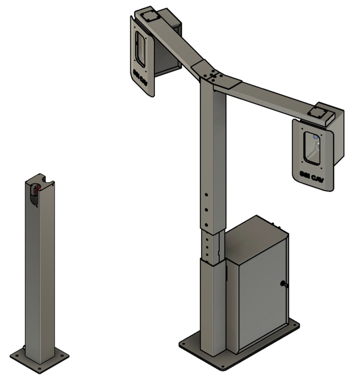
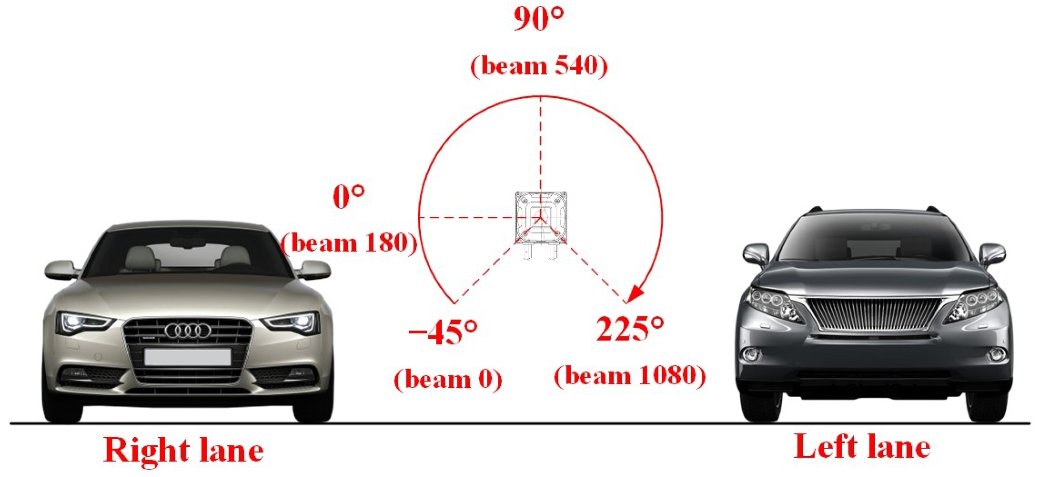
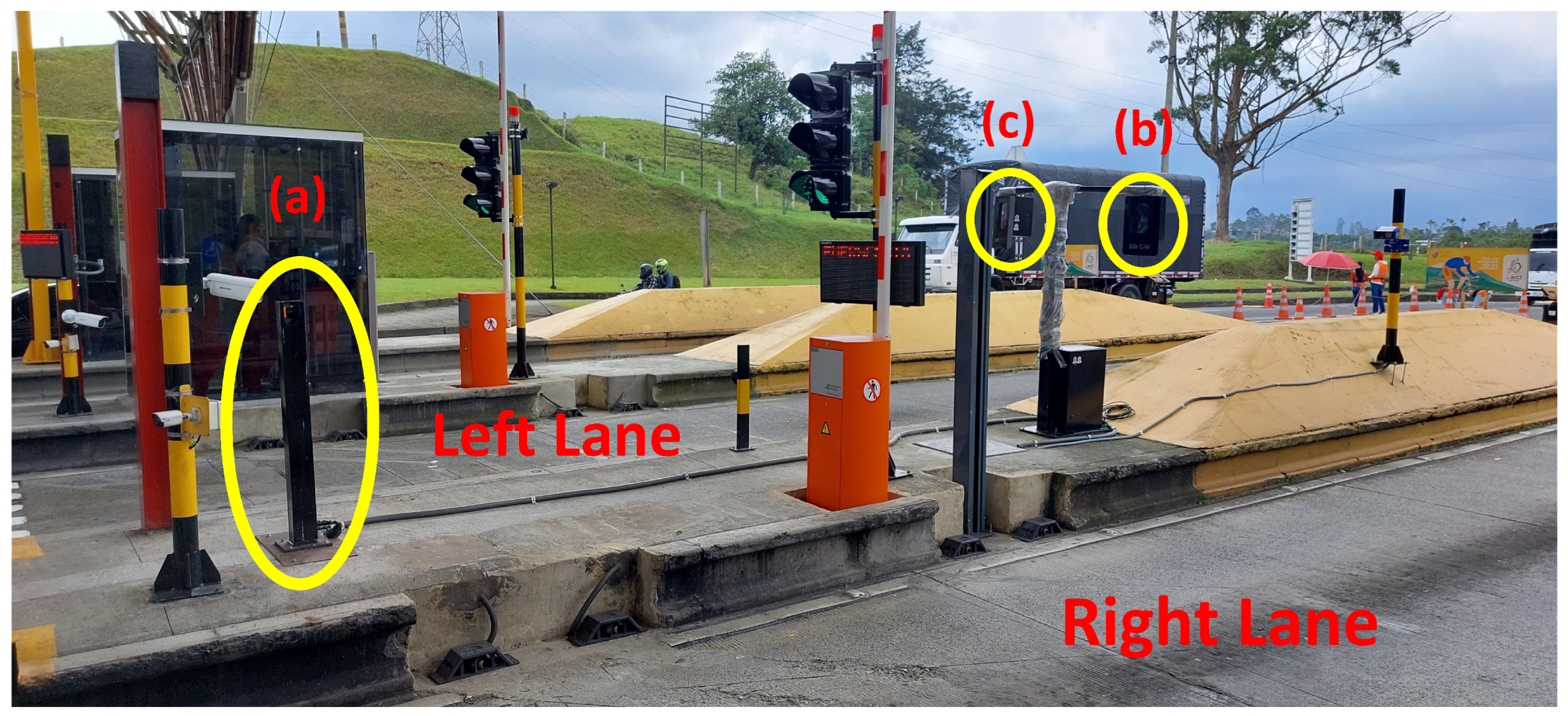
The system uses a robust physical platform composed of a Hokuyo UTM-30LX 2D LiDAR [52], two Stalker stationary speed radars [53], and two Prosilica GT1290C video cameras [54], all connected to a fanless industrial mini-PC housed in an aluminum case, as shown in Figure 1a. This setup enables simultaneous monitoring of two adjacent toll lanes. As illustrated in Figure 1b, each lane is equipped with a dedicated camera and speed radar, while a single LiDAR unit covers both lanes with its wide 270 ° scanning angle.
The laser sensor is positioned between two adjacent lanes, directing its beams toward the sides of passing vehicles to generate detailed 3D models of their lateral surfaces (see Figure 2). To ensure accurate data acquisition, the operator must keep distances B and C between 0.5 m and 2.5 m, ensuring that no objects obstruct the laser’s line of sight to either the vehicle or the ground. The installation height A should allow full coverage of the wheels. To maintain point cloud density, the system requires vehicle speeds to remain below 40 km/h; handling faster traffic conditions would require higher sampling-rate sensors. Continuous vehicle motion through the scanning zone is also essential to prevent data distortion from unexpected stops.
Speed radars should be installed 5 to 10 m from the laser sensor and aligned toward the lane center, ensuring their beams intersect the laser’s field of view in the center of the lane (see Figure 1b). Visible-spectrum cameras capture images as vehicles cross the laser beam, and operators must ensure proper focus to enable reliable license plate recognition. They should be positioned as perpendicular as possible to the plate surface. All components must be housed in weather-protected enclosures to ensure long-term durability, consistent performance, and interference-free data acquisition.

Design and Construction of the Physical Structure

The system’s physical structure ensures reliable performance under high-demand tolling conditions. Made from high-strength, corrosion-resistant steel, its modular design enables easy transport, installation, and reconfiguration. It includes a 1-meter galvanized pole for mounting the laser sensor, an IP65-rated industrial computer and electronics enclosure, and two upper arms with weatherproof housings for cameras and radars. Internal conduits and military-grade connectors protect wiring and ensure electrical stability. With ± 30 cm adjustable height and angular alignment mechanisms, the CAD-modeled structure (prototyped in Figure 3) offers a durable and flexible platform for advanced vehicle detection and classification.

3.2. Software Description

The system comprises interconnected software modules that process data from integrated sensors to generate 3D point clouds of passing vehicles. These are then analyzed and classified into predefined categories using advanced computer vision and pattern recognition techniques. It also includes a module for automatic license plate recognition to manage key vehicle information. Classification results and plate images are stored in structured formats and transmitted to the management system for efficient analysis and use. Figure 4 illustrates the system architecture, and Table 4 details the functional requirements. The software was developed in Python 3.6.9, using the Point Cloud Library (PCL) [56] v1.10.1 for point cloud processing. The following sections present the technical details of each module.
This section describes the architecture and functional modules of the proposed system, based on the structure presented in Figure 4. Each subsection from Section 3.2.1 to Section 3.2.7 corresponds to a specific component in the system’s workflow, including the graphical interface, data acquisition, preprocessing, vehicle segmentation, feature extraction, classification, and plate recognition.
It is worth noting that the Automatic License Plate Recognition (ALPR) module, described in Section 3.2.7, is part of the overall system but is operationally decoupled from the point cloud processing and classification pipeline. While the classification of vehicles is based on LiDAR data and trained with a dedicated dataset (detailed in Section 3.2.6), the ALPR module uses video imagery and a separate dataset, and its outputs are used primarily for record-keeping and traceability rather than influencing classification outcomes.
The organization of the subsections reflects both the logical flow of the system architecture and the functional independence between modules, facilitating clarity in presentation and alignment with the system’s real-world implementation.

3.2.1. Configuration and Processing Graphical Interface

The designed and implemented graphical user interface (GUI) facilitates intuitive and efficient interaction with the proposed system’s data acquisition and processing components. The GUI functions as an integrated control panel for configuration and operational monitoring, allowing real-time management of system parameters according to the specific characteristics of each deployment scenario.
The GUI architecture consists of three main modules: “hardware configuration”, “software configuration”, and “operational control”. Configuration modules must be completed before system activation to ensure synchronized sensors and initialization of parallel processing threads.
The “hardware configuration” module provides interfaces for assigning and validating serial communication ports for the LiDAR scanner, Doppler speed radars, and video cameras. It also allows users to associate sensors with specific toll lanes and define their operational ranges. Additional functionalities include real-time device status indicators, automatic hardware detection routines, and persistent error logging mechanisms.
The “software configuration” module allows fine-grained customization of algorithmic parameters. Key settings include the following: definition of the region of interest (ROI) through angular and distance thresholds for each lane (to enable valid sample selection and distance-based filtering); thresholds for statistical outlier removal; selection of radius parameters for surface normal estimation, keypoint detection, and FPFH computation; configuration of the clustering algorithm for BoW encoding; kernel selection for the support vector machine classifier; and activation of the automatic license plate recognition module. Furthermore, the user can specify storage paths for structured data logging and define host parameters for encrypted data transmission.
All GUI modules operate under a multithreaded execution model, in which each component runs as an independent subprocess. This design ensures non-blocking user interactions and parallel data processing, optimizing computational performance and ensuring real-time system responsiveness, even under conditions of high traffic density.
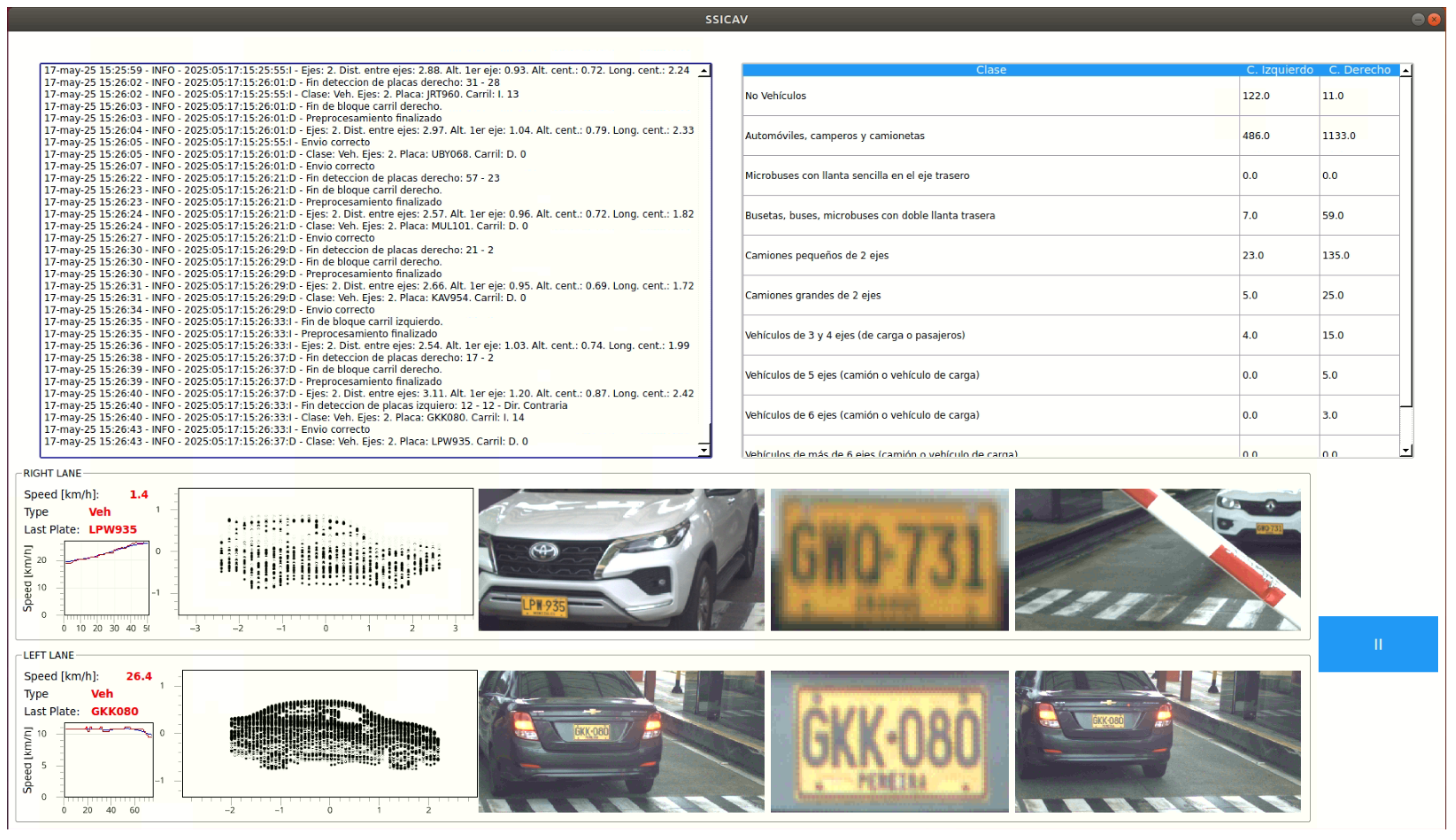
Figure 5 illustrates the GUI operational screen, enabling real-time system performance supervision. Key metrics, such as the number of vehicles processed, classification results, estimated vehicle speed, detected license plate, and the point cloud and photographic record of the latest vehicle for each lane, are updated dynamically. This comprehensive display provides high situational awareness and supports rapid decision-making in the field.
The GUI fully complies with the functional requirements outlined in Table 4. It enables in situ system customization and robust interaction with all sensing and processing modules, contributing to its overall usability, adaptability, and scalability across heterogeneous operational environments.

3.2.2. Data Acquisition

In the data acquisition stage, the system performs sensor configuration and data capture and determines whether the acquired data contains valid information corresponding to a vehicle object. Figure 6 shows the block diagram of the data acquisition module. The laser rangefinder interface uses the HokuyoAIST library [57,58], while communication with the speed sensors relies on the pySerial module, version 3.4 [59]. Similarly, the system establishes communication with the cameras through the Vimba API provided by the manufacturer, Prosilica [60].

Valid Sample Selection

This process detects when a vehicle enters the laser sensor’s field of view and initiates a new laser data block that captures all beam measurements during the vehicle’s passage, excluding those associated with zero velocity. For each lane, the system defines a ROI as a conical area in polar coordinates, bounded by specific radial and angular limits (see Figure 7). The ROI excludes irrelevant surfaces such as the ground and nearby obstacles. Once defined, the system continuously monitors objects within the ROI and validates their movement using speed data. It initiates a new data block upon detecting motion and triggers image capture for license plate recognition. The point cloud generation begins once the object exits the ROI and the system has accumulated sufficient valid laser measurements.

3.2.3. Creation of the Point Cloud

This stage processes the laser data block acquired in the previous step to generate a point cloud representation of the vehicle. The laser scanner operates on a polar coordinate plane in which 0 ° is oriented horizontally toward the right lane (see Figure 8). It captures measurements across an angular range from 45 ° to 225 ° , covering both lanes. The scanner operates at 40 samples per second (SPS), completing a full rotation every 25 milliseconds. With an angular resolution of 0 . 25 ° , each scan yields 1081 data points: 541 corresponding to the right lane and 540 to the left.
After receiving the laser data and the corresponding velocity vector, the system generates a 3D scene representation using a Cartesian coordinate system: Z represents height, X represents length, and Y represents width. Scan data in polar coordinates r , θ are converted to Cartesian coordinates Y , Z using the Equation (1). Angular values for the right lane range from 45 ° to 90 ° , and for the left lane, from 90 . 25 ° to 225 ° .
Y = r c o s π 180 θ , Z = r s i n π 180 θ
To compute the X coordinate of each point in the cloud, the system uses the vehicle’s speed vector and processes it to reduce abrupt variations caused by real-time measurement noise. This preprocessing applies a first-order Kalman filter and smoother [61,62,63,64], assuming constant velocity in a linear motion model.
Equation (2) defines the model’s state transition equation for both the Kalman filter and the smoother, and describes the state observation equation, where x k is the state vector at time k, composed of the vehicle’s position p and velocity v; F is the state transition matrix; w k is the process noise vector; δ t is the laser sampling interval, z k is the observation vector at time k, represented by the measured vehicle velocity; H is the observation or output transition matrix; and v k is the measurement noise vector.
x k + 1 = F x k + w k , p k + 1 v k + 1 = 1 δ t 0 1 p k v k + w k z k = H x k + v k , v k = 0 1 p k v k + v k
The covariance matrices are defined according to the methodology described in [64], as shown in Equation (3), where Q is the process noise covariance matrix, R is the measurement noise covariance matrix, P 0 is the initial state covariance matrix, x 0 is the model’s initial state vector, and v 0 is the vehicle’s velocity at the first sample.
Q = δ t 3 3 δ t 2 2 δ t 2 2 δ t , R = 1 , P 0 = 1 0 0 1 , x 0 = 0 v 0
Kalman filtering is a forward iterative prediction process that begins with the first sample of the speed vector. Equation (4) describes the filter, where x ^ k is the predicted state vector at time k, P ^ k is the predicted state covariance matrix, P k is the estimated state covariance matrix, and K k is the Kalman gain matrix. The state vector x k includes the filtered or estimated vehicle speed.
x ^ k = F · x k 1 P ^ k = F · P k 1 · F T + Q K k = P ^ k · H T · H · P ^ k · H T + R 1 x k = x ^ k + K k · z k H · x ^ k P k = P ^ k K k · H · P ^ k · H T + R · K k T
The Kalman smoother processes filtered velocity by a backward iterative update process that starts from the last estimated state vector and the last state covariance matrix computed by the Kalman filter. Equation (5) describes the smoother, where K ˜ k is the Kalman gain of the smoother, x ˜ k is the smoothed state vector, and P ˜ k is the smoothed state covariance matrix. The smoothed state vector x ˜ k includes the smoothed speed value.
K ˜ k = P k · F T · P ^ k + 1 1 x ˜ k = x k + K ˜ k · x ˜ k + 1 x ^ k + 1 P ˜ k = P k + K ˜ k · P ˜ k + 1 P ^ k + 1 · K ˜ k T
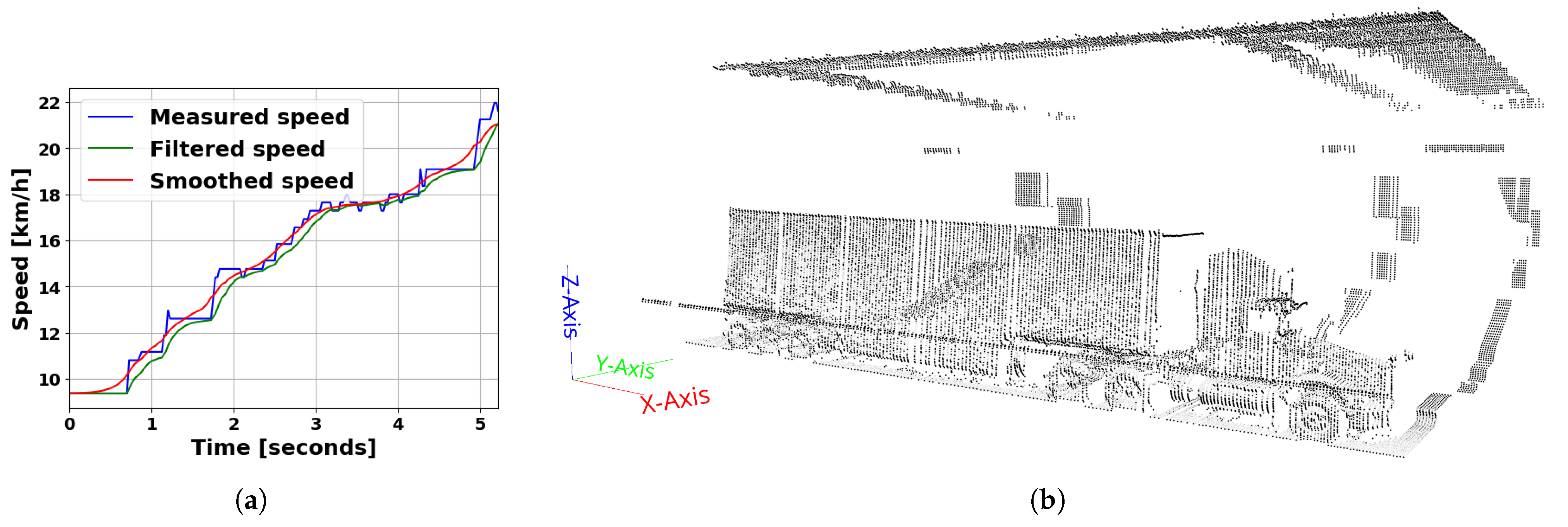
Figure 9a shows an example of the obtained smoothed speed profile. Equation (6) computes the longitudinal X coordinate, where X p r e v is the previous coordinate (initialized to 0) and f i l t e r e d _ v e l o c i t y is the current smoothed speed.
X = X p r e v + f i l t e r e d _ v e l o c i t y · δ t
These transformations generate a 3D matrix that defines the vehicle’s point cloud. Figure 9b illustrates an example of a 3D point cloud. However, for vehicles exceeding 25 km/h, the fixed sampling rate of the LiDAR can generate low-resolution point clouds, with intervals between scans greater than 18 cm. To address this, linear interpolation is applied between successive scans when the average speed exceeds 25 km/h, which improves the point density for speeds up to 40 km/h. The following processing stages receive the generated point clouds.

3.2.4. Point Cloud Preprocessing

The point cloud preprocessing stage aims to generate a refined vehicle representation by removing background elements, ground surface data, and noise, and correcting tilt distortions. Figure 10 shows the general block diagram of this process. The following subsections describe in detail the four stages illustrated in the figure.

Distance Filtering

Distance-based filtering removes irrelevant data, such as pedestrians, background structures, other roadside equipment, or vehicles in adjacent lanes. The filter applies thresholds along height (Z-axis) and depth (Y-axis). As shown in Figure 11a, the red area represents the region of interest defined by user-configurable Z and Y boundaries.
The user adjusts the threshold values according to the specific installation parameters of the laser sensor, using lane width and maximum vehicle height as the main criteria. Figure 11b shows the point cloud from Figure 9b after applying distance filtering. The resulting data isolates the target vehicle and the road surface within the corresponding lane, effectively removing background elements.

Ground Surface Extraction

A standard method for segmenting point clouds involves estimating parametric models, such as planes, to isolate structural elements. This stage applies a plane extraction algorithm based on RANSAC to identify and remove the road surface, following the implementation described in [26,27]. The ground is assumed to be the dominant plane, perpendicular to the Z axis and defined by Equation (7). The algorithm selects the plane with the highest number of inlier points within a predefined distance threshold (5 cm) and angular deviation ( 10 ° ) from the model, then removes those points from the point cloud. With a maximum of 5000 iterations, the method proved effective, as illustrated in Figure 12, where the extracted ground (in red) is separated from the vehicle (in black). Reference [55] describes the details of the implemented algorithm.
a x + b y + c z + d = 0

Tilt Angle Correction

The next step involves estimating the tilt angles between the ground plane and the XY plane, which result from any inclination of the laser sensor during installation. These angles are computed using Equation (8), based on the coefficients (a, b, and c) of the ground plane model from Equation (7), since these coefficients represent the plane’s normal vector. In this context, θ x denotes the inclination around the X-axis, and θ y around the Y-axis.
θ x = arctan b c , θ y = arctan a c
This stage rotates each point x , y , z in the point cloud using the Euclidean rotation matrices R x θ x and R y θ y , as defined in Equation (9).
R x θ x = 1 0 0 0 cos θ x sin θ x 0 sin θ x cos θ x , R y θ y = cos θ y 0 sin θ y 0 1 0 sin θ y 0 cos θ y

Statistical Filtering

Statistical filtering removes noise from the point cloud, such as isolated points caused by ambient dust or measurement uncertainty. The filter implementation uses the algorithms described in [26,65]. The method calculates the average distance d ¯ from each point to its k nearest neighbors. It retains only those within a range of μ ± α σ , where μ and σ are the global mean and standard deviation of all average distances. Reference [55] describes the details of the filtering algorithm implemented in this work. Equation (10) defines the resulting filtered cloud 𝒫 * .
𝒫 * { p i * 𝒫   | ( μ α · σ ) d ¯ i * ( μ + α · σ ) }
After several experiments with different point clouds, the nearest neighbor value k = 50 and a filtering factor α = 2.5 produced satisfactory results, effectively removing numerous outlier points in each cloud tested. Figure 13 shows the results with the filtered cloud in black and the removed points in red, highlighting the improvement in surface homogeneity and the removal of scattered noise.

3.2.5. Feature Extraction

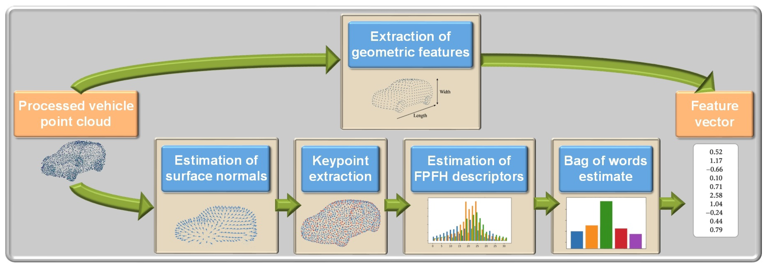
The next step involves extracting relevant features from the point cloud, which serve as input to the classifier described in Section 3.2.6, whose objective is to determine the vehicle type automatically. Figure 14 shows a general diagram of the feature extraction process. This stage has two main goals: to reduce the volume of data processed in subsequent stages and to enhance classification efficiency. The Cartesian coordinates x , y , z of thousands of points offer limited discriminative power and are computationally expensive to process. The feature types extracted to address this are as follows: (1) global geometric properties of the vehicle (e.g., height, length); (2) a BoW representation derived from FPFH, a local 3D descriptor computed using surface normals and keypoints from the point cloud. The following subsections describe the extraction process for each feature type in detail.

Estimation of Surface Normals

Three-dimensional point clouds from range sensors capture sampled surfaces of real-world objects but lack information about surface orientation and curvature. To recover this geometric context for subsequent analysis, surface normal estimation is required. Extracting surface normals is a computationally efficient and robust technique, particularly effective against discontinuities in raw range data [66,67,68].
Implementing the surface normal extraction method uses the algorithms described in [26], which employ Principal Component Analysis (PCA) to estimate surface normals by fitting a tangent plane to the local surface around each point of interest. This results in a least-squares approximation of a plane in the neighborhood of a point p i . This approach reduces the normal estimation problem to the eigenvalue and eigenvector analysis of the covariance matrix computed from the point’s local neighborhood.
Equation (11) shows the covariance matrix C i R 3 x 3 computation for a point p i , where k is the number of neighboring points considered within a defined radius r, and p ¯ i denotes the 3D centroid of this neighborhood. The covariance matrix’s eigenvalues λ j and eigenvectors v j represent the local geometric structure. If the eigenvalues satisfy 0 λ 0 λ 1 λ 2 , then the surface normal n i is defined as the eigenvector v 0 associated with the smallest eigenvalue λ 0 .
C i = 1 k n = 1 k p n p ¯ i · p n p ¯ i T , p ¯ i = 1 k n = 1 k p n , C i · v j = λ j · v j , j 0 , 1 , 2
However, the previous method does not determine the sign of n i , meaning the orientation of the normal vector remains undefined. The normals must comply with Equation (12) to ensure their orientation is consistently toward the viewpoint, i.e., the laser position. In this expression, v p represents the viewpoint, defined as a central point on the XZ plane of the vehicle’s point cloud, located at a distance equal to or greater than that of the LiDAR sensor.
n i · v p p i > 0
As noted in [26,69], choosing an appropriate scale factor for r or k value is essential for accurate surface normal estimation and feature extraction in 3D point clouds. The optimal choice depends on task requirements and data characteristics, and may involve techniques such as automatic selection, sensitivity analysis, or empirical testing [24,70,71].
The neighborhood scale factor depends on the required level of geometric detail. Smaller values are needed to capture fine features like edge curvature, while larger values are suitable for less detailed applications. However, small scales must align with the point cloud resolution. For instance, in vehicle point clouds captured at 25 km/h, where point spacing along the X-axis averages 18 cm, the radius r should be greater than that spacing.
Based on this, the neighborhood estimation used a radius of 36 cm, and the viewpoint was placed 5 meters away from the point cloud, perpendicular to the XZ plane and centered with respect to the scene.

Keypoint Extraction

The next step is to identify keypoints: stable, distinctive, and well-defined points within the point cloud. Selecting these reduces the data volume for classification and, when combined with local 3D descriptors, enables a compact and informative representation of the original point cloud [72].
Standard keypoint detectors include voxel sampling, uniform sampling [73], Harris3D [74], SURF 3D [75], NARF [76], and ISS [77]. This work adopts the uniform sampling method, known for its efficiency, repeatability, and low computational cost [73]. The approach subdivides the point cloud into 3D voxels of a predefined radius and selects the point closest to each voxel’s center as a keypoint.
Since wheels are key features for vehicle classification and typically exceed 60 cm in diameter, a voxel radius of 10 cm was chosen for keypoint extraction. This value preserves essential structural details while reducing the number of points by over 80 % .

Estimation of FPFH Descriptors

The original format of a point cloud provides Cartesian coordinates x , y , z relative to the sensor’s origin. However, this raw representation can lead to high ambiguity in applications such as automatic vehicle counting and classification, where a system must compare multiple point sets. To address this, the system uses local descriptors to capture the geometric structure around keypoints, enabling more reliable feature comparison. These descriptors must provide a compact, robust, and invariant representation, resilient to noise and occlusions [78].
Based on the previous definition of local descriptors, the surface normals estimated in Section 3.2.5 for the keypoints extracted in Section 3.2.5 are local descriptors, as they capture geometric information from the neighborhood of each point of interest. However, the geometric detail they provide is relatively limited in terms of the level of classification required. To address this, a more advanced local descriptor called FPFH [78] was selected, which builds upon the information provided by surface normals.
The feature extraction method used for the FPFH descriptor, presented in [78], is based on a simplified version of the original Point Feature Histogram (PFH) algorithm [79,80]. This approach significantly reduces the original method’s computational complexity, making it suitable for real-time applications while preserving most of PFH’s descriptive power. The method calculates the FPFH descriptor by analyzing the angular relationships between surface normals at a set of keypoints and their neighbors [26].
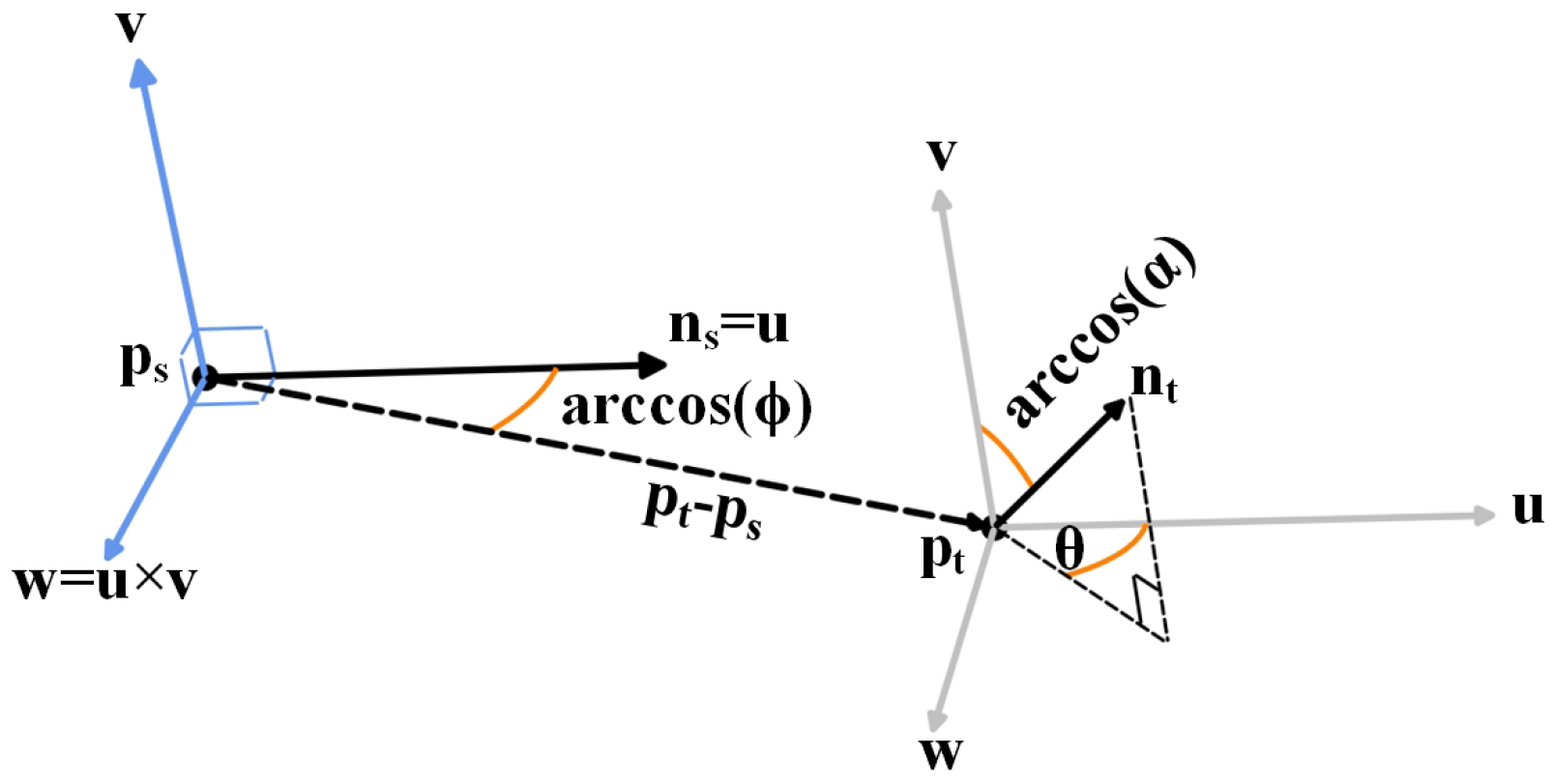
The process begins by estimating angular features α , ϕ , θ between a keypoint p i and its k nearest neighbors within a specified radius r. For each pair of points p i and p j , the method defines a Darboux reference frame at one of the two points, where p j is the j-th neighbor of p i , as shown in Figure 15. These angular tuples represent the relative geometry between pairs of surface points and reduce the feature space from 12 (i.e., the x, y, and z coordinates, and normals of the keypoint and its j-th neighbor) to 3 dimensions.
Unlike PFH, which calculates all possible point-pair interactions in the neighborhood, FPFH limits computations to keypoint-neighbor pairs, offering a substantial speedup. These angular values are then grouped into histograms with 11 bins per dimension, producing a Simplified PFH (SPFH) for each keypoint. In a final step, the method weights the SPFH values of the neighboring points and aggregates them to form the complete FPFH descriptor, as expressed in Equation (13), where ω j denotes the distance between the query point p i and a neighboring point p j .
F P F H p i = S P F H p i + 1 k j = 1 k 1 ω j · S P F H p j
The final output of this stage is a set of 33 normalized values (ranging from 0 to 1, or 0 % to 100 % ) for each keypoint in the point cloud. Figure 16 displays the histograms of five randomly selected keypoints from a six-axle truck point cloud. The figure shows an apparent similarity between points 2 (green), 3 (yellow), and 5 (magenta), all located on the flat cargo surface parallel to the XZ plane. In contrast, points 1 (blue) and 4 (cyan), located respectively on the fender and a tire, exhibit distinct histogram shapes.
To determine the radius r used in the computation of the FPFH descriptor, the system adopts the hierarchical neighborhood strategy proposed by Rusu [26], which relies on a dual-ring approach. This method defines two distinct radii, r 1 < r 2 , to compute two separate layers of feature representations for each keypoint p i . The first layer captures surface normals using radius r 1 , as described in Section 3.2.5, while the second computes the FPFH features using radius r 2 . In this implementation, the system sets the surface normal radius to 36 cm, and it defines the FPFH radius as 1.2 times r 1 , i.e., 43 cm, to ensure that feature extraction remains within the scale of relevant vehicle structures such as wheels.

Bag-of-Words Estimate

Three-dimensional local descriptors capture distinctive geometric features within point clouds, offering robustness and adaptability for object analysis and recognition tasks [28]. However, their quantity varies with point cloud size, often ranging from hundreds to thousands, introducing inconsistency across different vehicles and complicating direct comparison and classification [81]. Consequently, a BoW model standardizes representation [28,29,30]. This approach clusters similar local descriptors into “visual words” or “bags,” yielding a compact, fixed-length vector suitable for classification. The following outlines the method proposed [82,83,84,85,86,87]:
  • A visual dictionary is first constructed by clustering FPFH descriptors extracted from a training dataset using methods like k-means.
  • Each descriptor is assigned to its nearest visual word based on similarity to cluster centroids.
  • Finally, for each point cloud, the frequency of occurrence of each visual word is counted, producing a BoW histogram that summarizes the distribution of local geometric features.
The number of visual words (or clusters) depends on the application and the dataset’s characteristics [81]. This value is fixed and must be large enough to capture meaningful variations while avoiding overfitting to noise [88]. The optimal number is selected experimentally to balance the representation’s discriminative power and generalization capacity [84]. Section 4 of Results evaluates different visual dictionary sizes to analyze their impact on classification performance.
The final output of this stage is a set of N values ranging from 0 to 1 ( 0 % to 100 % ) for each point cloud, where N represents the number of visual words. Figure 17 shows a histogram (right) generated using five visual words for a single point cloud, and a visualization (left) of the spatial distribution of keypoints assigned to each word across the entire vehicle point cloud.
The system constructs the visual vocabulary using the Mini-Batch K-means algorithm, which improves computational efficiency by processing small random subsets in each iteration [89,90]. Although this method may slightly reduce clustering accuracy, it performs reliably in large-scale settings. Two initialization strategies were tested: K-means++, which improves convergence via probabilistic seeding, and random selection of initial centroids.

Extraction of Geometric Features

The system classifies vehicles into eight distinct categories, as shown in Table 3, based primarily on the number of wheels in contact with the ground and overall vehicle dimensions. The system uses a geometric feature extraction method to improve classification efficiency, following approaches similar to those in [46,91]. The geometric features extracted from the point cloud are illustrated in Figure 18 and include the following:
  • Number of keypoints: The total number of extracted keypoints indicates the size of the point cloud.
  • Vehicle length: Measured as the distance between the farthest points along the X-axis.
  • Vehicle height: Defined as the vertical span of the point cloud along the Z-axis.
  • Number of axles with tires on the ground: The method excludes lifted axles of freight vehicles with three or more axles.
  • Distance between front and rear axles: Calculated as the distance along the X-axis between the centers of the front and rear wheels.
  • Vehicle height at the front axle: The vertical distance along the Z-axis at the front axle’s location.
  • Front tire diameter: Considering that most vehicles have tires of uniform size.
The output of this stage is a set of seven values that describe the geometric properties of each point cloud. Combined with the N visual words obtained in the previous section, they form the complete feature set used in the following classification stage.
However, due to the significant variance in the magnitudes of geometric features, feature scaling is necessary to ensure equal contribution to the classification model and improve performance [92]. Scaling enhances the convergence of optimization algorithms, reduces classification errors in scale-sensitive models like SVM and KNN, and improves consistency and interpretability, especially when dealing with heterogeneous real-world data.
Section 4 of the Results evaluates four scaling techniques using the Scikit-learn library [90] to assess their impact on classification performance. The Standard scaler removes the mean and scales the data to unit variance by dividing by the standard deviation. The MaxAbs scaler divides each value by its maximum absolute value, preserving sparsity. The MinMax scaler normalizes features to a fixed range (e.g., 0 ,   1 ). The Robust scaler subtracts the median and scales by the interquartile range (IQR), making it resilient to outliers.

Axle Detection and Counting

As shown in Figure 18, the system can directly calculate the vehicle’s length and height as the difference between the minimum and maximum coordinates along the X and Z axes, respectively. Estimating the remaining geometric features requires identifying the positions of the axles.
To achieve this, a horizontal slice of the point cloud is extracted at a height D above the ground, capturing only the lower section of the wheels while excluding the vehicle body (see Figure 19). Euclidean clustering is then applied to segment candidate axle regions, using parameters such as the minimum and maximum number of points per cluster ( m i n c s , m a x c s ) and a search radius d t h .
The method increases D when it detects three or more axles or when the vehicle height exceeds the threshold h t h ; conversely, it reduces D if it detects fewer than two axles, repeating the process accordingly. The method validates clusters as axles only if they meet the following conditions:
  • The height of the cluster must be at least 50 % of D; otherwise, the cluster may represent noise or another part of the vehicle.
  • The cluster length (interpreted as wheel diameter) must exceed the threshold w m i n to exclude small or fragmented clusters.
  • The cluster’s minimum Z coordinate must lie within a tolerance t t h from the ground level (i.e., the minimum Z of the entire cloud), ensuring that the axle is in contact with the road and not lifted.
Once the algorithm identifies valid axles, it determines how many are in contact with the ground, locates the positions of the first and last axles, and calculates derived characteristics such as vehicle height at the front axle, inter-axle distance, and wheel diameter.
Extensive testing led to selecting the following parameters: D = 12 cm, m i n c s = 20 points, m a x c s = 5000 points, d t h = 25 cm, h t h = 1.8 m, w m i n = 30 cm, and t t h = 5 cm. Figure 20 shows an example of identified axle clusters.

3.2.6. Automatic Classifier

The automatic classification stage uses the histogram of the N visual words and the extracted geometric descriptors as input. Based on this information, the classifier determines the corresponding vehicle category. Researchers have applied various methods in point cloud classification, including neural networks [25,33,34], Bayesian networks [35], k-nearest neighbors (KNN) [93], and SVM [31,32]. This work adopts and trains an SVM classifier because it effectively handles high-dimensional and complex data from point clouds. SVMs are well-suited for classification tasks even when the data is not linearly separable, offering robust performance under data variability [31,32].
While SVMs are inherently binary classifiers that determine the optimal hyperplane separating two classes, this implementation extends their functionality to multiclass problems using the One-Versus-Rest (OVR) strategy [94,95,96]. This approach decomposes a multiclass problem with K classes into K binary classification tasks, each distinguishing one class from all others.
For each class C k , a binary SVM model is trained to separate the samples of class C k (labeled as + 1 ) from the rest (labeled as 1 ), solving an individual optimization problem under the maximum margin principle. The predicted class for each sample corresponds to the classifier with the highest decision function value.
A key strength of SVM classifiers lies in kernel functions, which allow nonlinear relationships to be modeled by implicitly mapping the input data to higher-dimensional spaces without explicitly computing the transformation. Section 4 of the Results evaluates three commonly used kernel functions described below: (i) the linear kernel, suitable for linearly separable data; (ii) the polynomial kernel, which captures nonlinearities through adjustable degree and bias terms; (iii) the Radial Gaussian Basis Function (RBF) kernel, which maps the data to an infinite-dimensional space to capture complex nonlinearly separable patterns.
Finally, the classification model follows a structured pipeline composed of the following stages:
  • Dataset construction: This process begins by selecting a representative subset of point clouds from a larger dataset as the basis for model development.
  • Class labeling: The annotation process assigns each point cloud a class label corresponding to its vehicle category. A Label Encoding scheme then converted these categorical labels into unique integer identifiers to enable compatibility with the classification algorithms used in subsequent stages.
  • Data partitioning and class balancing: The labeled subset is partitioned into training and validation sets using a stratified approach to preserve class distribution. Additionally, class balancing techniques are applied when necessary to mitigate the effects of class imbalance and ensure fair model training.
  • Visual vocabulary generation: The process constructs a visual dictionary using the Mini-Batch K-means algorithm for FPFH descriptors extracted from the training samples. Each point cloud is then represented as a histogram of visual word occurrences, capturing local geometric patterns in a compact, fixed-length format.
  • Geometric feature extraction and normalization: The system extracts seven global geometric descriptors from each point cloud and normalizes them using different scaling strategies to reduce the effects of scale variability and ensure balanced feature influence.
  • Feature vector construction: The normalized geometric features are concatenated with the corresponding BoW histogram to form a unified high-dimensional feature vector. This representation integrates global structure and local surface descriptors, enriching the input space for classification.
  • Model training and evaluation: The training phase applies SVMs with linear, polynomial, and Gaussian RBF kernels, allowing the model to capture linear and nonlinear class boundaries.
The classifier initially groups vehicles into the first four classes in Table 3, plus a fifth class corresponding to vehicles with three or more axles. Vehicles assigned to Class 5 are subsequently reclassified according to the number of axles, resulting in the eight vehicle categories.

Dataset Construction

The dataset creation process ensures data quality and representativeness by collecting range data, images, and speed records during a pilot deployment at a toll station. LiDAR and speed sensors generate the range data for constructing 3D point clouds, while high-resolution cameras capture synchronized images of each vehicle to support classification and manual verification.
The final dataset comprises over 360,000 vehicle samples, hierarchically organized by date and time to streamline access during processing. Each record included a text file containing range data (with a .out extension) and a synchronized PNG image captured during vehicle passage. Reference [55] provides more details about the dataset construction.

Class Labeling

The dataset’s labeling process is key to ensuring accurate vehicle classification. It involves assigning class labels to each object in the point clouds using automated and manual tools developed specifically for this task.
Labeling begins by reviewing point clouds to discard samples with excessive noise, incomplete captures, or distortions, and labeling them as “unidentified” or “distorted.” Camera images are inspected for clarity and used to verify key vehicle features, while speed data are compared to expected values to detect anomalies.
The labeling process assigns initial classes to point clouds based on geometric features and axle configuration, with visual confirmation provided by corresponding camera images. The final labeled dataset comprises 44 , 498 objects, most of which are light vehicles 73.63 % . Table 5 reports the sample distribution across classes, including auxiliary categories such as “non-vehicles” (Pedestrians, bicycles, motorcycles, or objects not subject to tolls under Colombian regulations; they are labeled as Class 0 to help the classifier ignore non-chargeable detections), “unidentified” (Point clouds with ambiguous features—e.g., unclear if a minibus has single or dual rear tires (Class 1 vs. 2), or if a two-axle truck fits Class 1, 3, or 4—making it impossible to assign a reliable label. These cases are excluded from training and evaluation), and “distorted” (Abnormally long point clouds caused when a vehicle stops in the laser beam of the reversible lane, and the radar falsely detects movement. We are evaluating sensor upgrades and algorithmic improvements to address this issue).
Unidentified samples included vehicles with unclear axle configurations, while distorted data resulted from laser beam obstructions, often due to congestion in a central reversible lane. The manual labeling process, being highly time-consuming and labor-intensive, limited the annotated portion of the dataset to 12.36 % ; nevertheless, the resulting subset proved reliable and representative.

Data Partitioning and Class Balancing

Due to the dataset’s significant class imbalance, particularly the predominance of Class 1 vehicles, a balanced subset was created to avoid bias and ensure reliable classification across all vehicle categories. The procedure excluded unidentified and distorted samples. Table 6 presents this balanced dataset, including the numeric codes assigned to each class. The process split the subset into 80 % for training and 20 % for validation.

3.2.7. Automatic License Plate Recognition

The Automatic License Plate Recognition (ALPR) module has three main stages. The first stage is plate detection, in which the system analyzes the input image to locate candidate regions likely to contain a license plate. The second stage is character recognition, where the characters within the detected regions are extracted and classified. The final stage is plate identification, consolidating the recognized characters into a validated license plate string.

License Plate Detection

The implementation adopts the method proposed in [97,98] for license plate detection. It combines Local Binary Pattern (LBP) descriptors with a cascade classifier trained using Adaptive Boosting (AdaBoost). The algorithm applies a multi-scale sliding window strategy to grayscale images and sequentially evaluates the candidate regions using weak classifiers.
LBP descriptors encode local texture by comparing each pixel to its eight neighbors, producing binary patterns converted into decimal values [99]. This process results in a compact and discriminative texture representation, facilitating further image analysis tasks. Figure 21 shows an example of the final LBP output.
To ensure robustness against plate size and position variations, the detection process is performed at multiple image scales using sliding windows. The method evaluates each candidate region through a 12-stage cascade of weak classifiers. Figure 22a shows the overall structure of the cascade classifier. This design enables early rejection of false positives, significantly reducing computational cost [100,101]. The process forwards the candidate regions that pass all stages to the character recognition module. Figure 22b shows some classifier stages, where four candidate regions, including the correct license plate, are ultimately observed.

Character Recognition

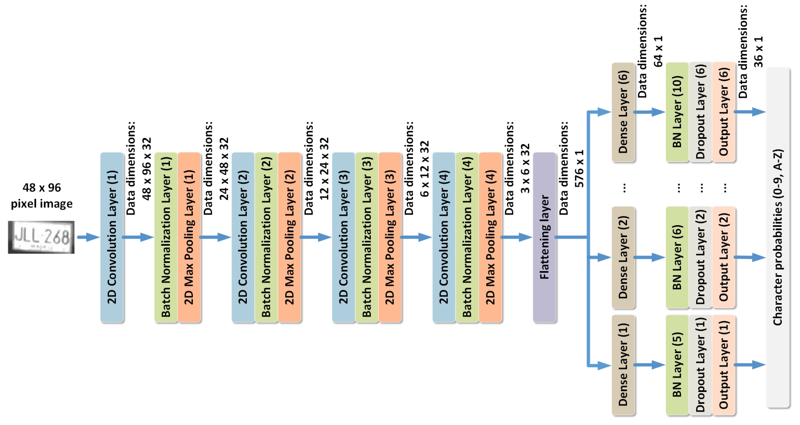
The character recognition module employs a deep learning architecture based on convolutional neural networks (CNN), following recent approaches reported in the literature [102,103,104,105,106,107]. The architecture illustrated in Figure 23 processes 48 × 96 -pixel grayscale images and extracts hierarchical features through multiple convolutional, pooling, and normalization layers. It includes six dense layers, one for each character, followed by SoftMax outputs over 36 classes (0 to 9, A to Z). Dropout regularization and batch normalization are applied throughout to prevent overfitting and stabilize training.
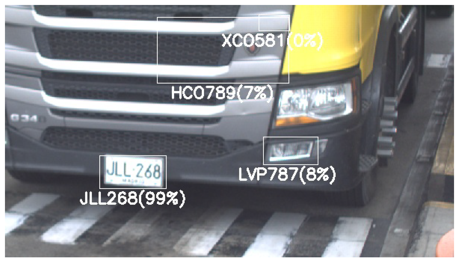
The classifier generates a probability distribution of the 36 possible classes for each of the six characters. The method constructs the final license plate by selecting the most probable class at each position. It calculates an overall confidence index by multiplying the individual probabilities. If this index exceeds a threshold of 0.3, the process accepts the image as a valid license plate. This value is determined experimentally, considering that a high value can discard valid plates and a lower value can generate false positives [108]. Figure 24 illustrates four initial candidates, of which only one is correct due to its high confidence index.

License Plate Identification

A single image captured per vehicle often results in high recognition error rates, mainly due to occlusions, poor lighting conditions, and imperfect synchronization between image acquisition and the vehicle crossing the laser beam. To address this, the system implements a multi-frame processing strategy to reduce recognition errors (see Figure 25).
Each video frame is processed independently for license plate detection and character recognition. Once a vehicle enters the scene, the system accumulates detected plate candidates across all subsequent frames until the vehicle crosses the laser beam. Due to noise and variability, some of these detections may contain incorrect characters.
A majority voting scheme is applied to assign a reliable license plate to each vehicle. The method selects the most frequently detected character across all valid frames for the six character positions. This voting mechanism increases robustness by compensating for isolated misclassifications, enabling the system to reconstruct a more accurate license plate even with partial occlusions or recognition noise.

Training the ALPR Classifiers

The evaluation used over 5000 high-resolution visible-spectrum vehicle images to assess the license plate recognition system. The annotation process manually labeled the license plate regions and their corresponding characters. The 12-stage cascade classifier was trained for plate detection using 2500 plate images and 4750 non-plate samples. The process reserved the remaining 2500 plate images for validation.
Detection performance was measured using the Jaccard coefficient, which compares predicted and ground-truth bounding boxes. The system considers a correct detection when J 0.5 . The model achieved 99 % accuracy in plate detection, with 200 false positives.
The character recognition process used 10,000 labeled character samples (A to Z, 0 to 9) and 4750 non-character images. The validation process evaluated 155 plates and accepted a result only when the system identified all the characters correctly. The system reached a 95.3 % accuracy, with 13 false positives. The training process used high-quality images captured under favorable conditions.

4. Results

This work’s main contribution is the development of the Vehicle Counting and Classification System, SSICAV. Designed as a comprehensive technological solution, SSICAV aims to optimize vehicle management at toll stations by integrating advanced sensing technologies and data processing capabilities.

4.1. Axle Detection and Counting Results

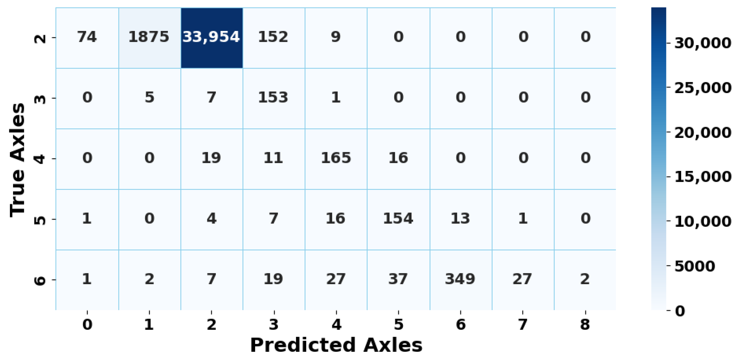
The evaluation treated the axle detection and counting module as a multiclass classification task, where each class corresponds to a vehicle with a specific number of axles, ranging from 2 to 6. Although the classifier could predict classes from 0 to 8, labels outside the valid range (i.e., 0, 1, 7, and 8) represent misclassifications. The analysis excluded vehicles with more than six axles due to their low representativeness in the dataset.
The system evaluation used a test set comprising 37,108 vehicle samples collected under real operating conditions. The overall accuracy reached 93.71 % , suggesting the system reliably estimates axle counts in most cases. However, performance varied across classes, partly due to the inherent class imbalance, as shown in Table 7. Two-axle vehicles accounted for more than 97 % of the dataset.
The confusion matrix in Figure 26 highlights the classifier’s ability to detect 2-axle vehicles correctly and reliably. However, the results reveal a systematic tendency to underestimate axle counts, particularly in higher axle configurations (e.g., 3 to 6 axles), which the model frequently misclassified.
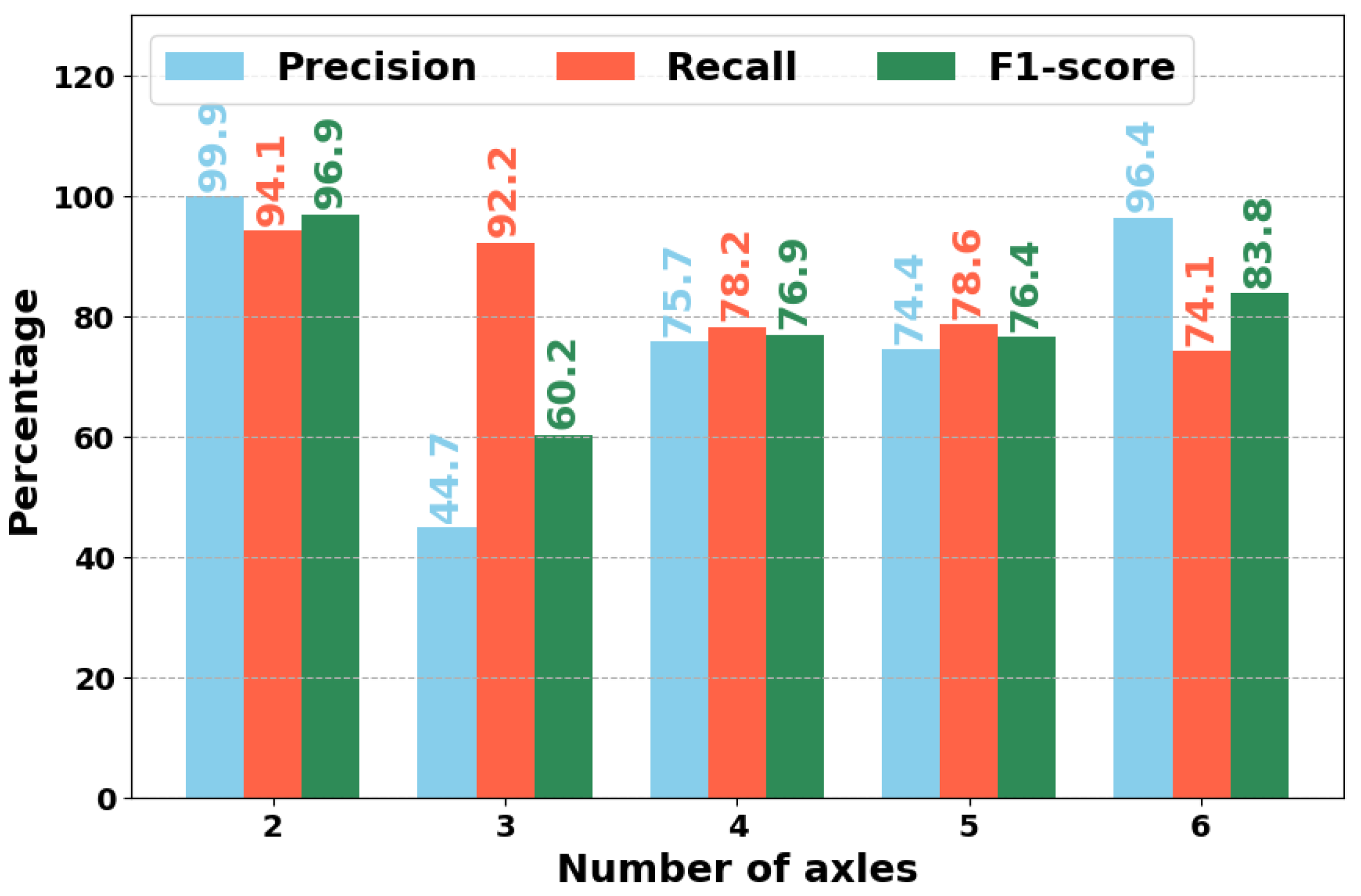
The metrics demonstrate that the axle classification model performs highly accurately under operational conditions. A global accuracy of 93.71 % and a weighted F1-score of 96.38 % reflect strong performance, especially for dominant classes like 2-axle vehicles. However, macro-averaged metrics (precision 43.46 % , recall 46.35 % , F1-score 43.81 % ) reveal significant class variability. This result is mainly due to reduced precision in underrepresented categories; for example, the 3-axle class achieved high recall ( 92.2 % ) but low precision ( 44.7 % ), indicating a substantial number of false positives.
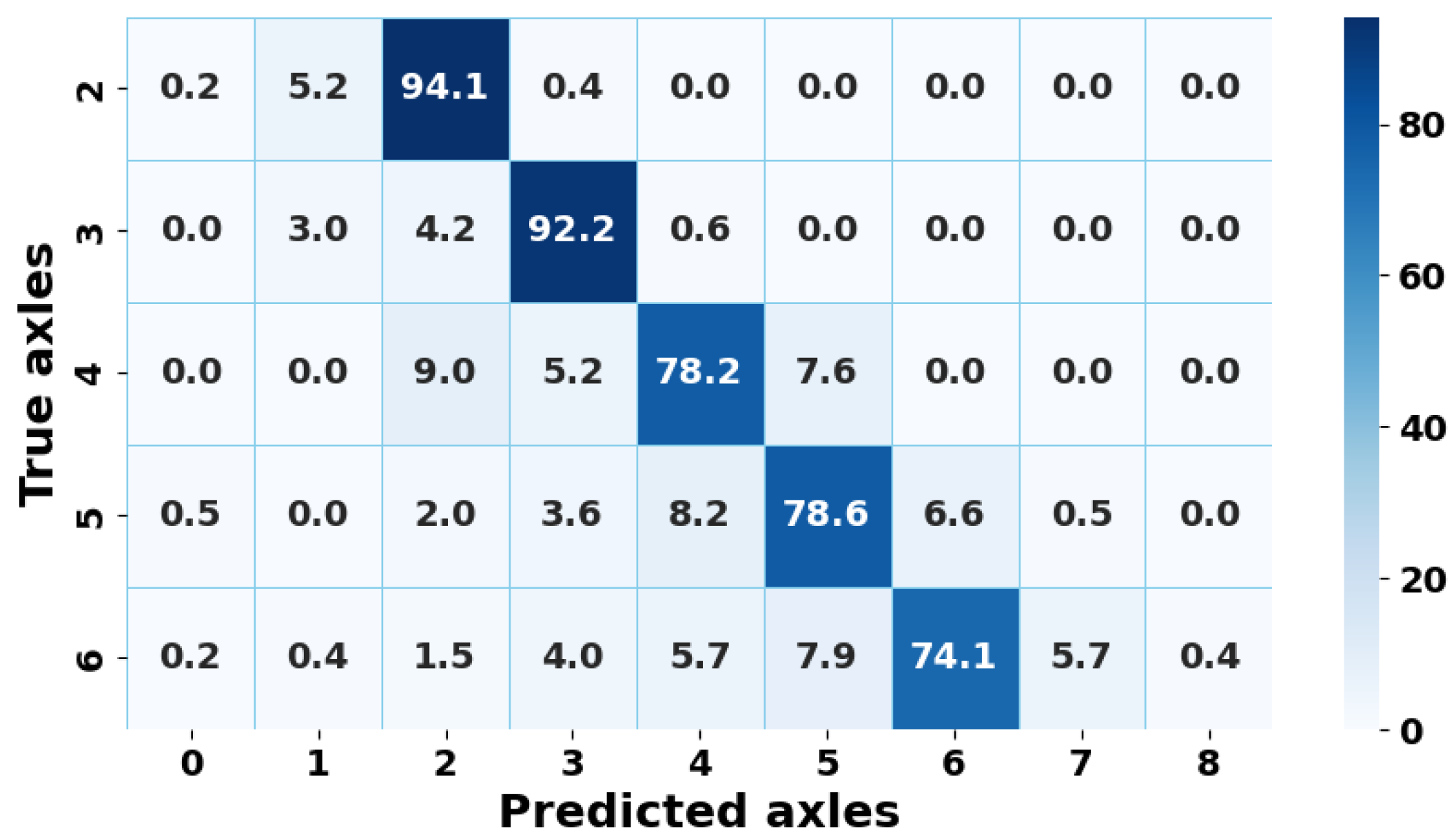
The row-normalized confusion matrix is shown in Figure 27 to facilitate class-wise performance analysis. The model achieved the highest recall for 2-axle vehicles ( 94.1 % ), which dominate the dataset. Interestingly, despite being a minority class, 3-axle vehicles exhibited a recall of 92.2 % , indicating that the model correctly recognized most true instances of this class. However, their precision was substantially lower ( 44.7 % ), revealing frequent false positives, primarily due to confusion with 2-axle vehicles. This imbalance suggests that while the model is sensitive to identifying 3-axle configurations, it struggles to discriminate them clearly from more common classes.
Figure 28 presents the complete set of per-class metrics. The 2-axle category achieved an F1-score of 96.9 % , reflecting consistently high precision and recall. In contrast, the 3-axle class obtained an F1-score of only 60.2 % , reflecting its low precision. The model exhibited more balanced behavior for classes with 4 to 6 axles, achieving F1-scores between 76.4 % and 83.8 % , although recall progressively declined as axle count increased. These patterns highlight the increased classification complexity in higher axle configurations, often compounded by partial occlusions and low data representativeness.
The analysis identified the sensor’s inability to fully capture some vehicles’ wheels, primarily due to traffic traveling close to the platform where the laser scanner was installed, as one of the main limitations in axle counting. This issue was more evident in long or multi-axle vehicles, and it worsened in reversible lanes due to irregular alignment and frequent stops near the sensor. These conditions led to systematic underestimation in complex axle configurations.
In summary, despite sensor visibility and class imbalance limitations, the model demonstrated high accuracy in detecting 2-axle vehicles and acceptable performance for configurations involving 3 to 6 axles. These results confirm the system’s applicability in toll plaza environments and point to potential improvements. The proposed approach addresses current limitations by combining infrastructure adjustments and sensing enhancements. It includes modifying the toll plaza divider to enable unobstructed laser beam passage and integrating complementary sensors, such as infrared or optical devices, to improve detection under low visibility and complex vehicle configurations.

4.2. License Plate Recognition Results

The annotation process excluded 10,938 images from the evaluation because insufficient resolution prevented visual identification of license plates in those cases. These images came from a dataset of 37,108 labeled samples corresponding to Class 1 through Class 5 vehicles. In the remaining 26,170 images, where the license plate region was sufficiently clear for manual labeling, the recognition performance was assessed based on the number of correctly identified characters per plate. This metric reflects the system’s effectiveness in accurately extracting alphanumeric sequences under real-world operating conditions.
On this subset, the system achieved a character-level accuracy of 95.25 % , measured as the proportion of individual characters correctly recognized across all plate positions. Full-plate recognition, defined as correctly identifying all six alphanumeric characters, was achieved in 79.94 % of the cases. The average normalized Levenshtein distance between the predicted and ground-truth strings was 0.28 , indicating that fewer than two character-level edits were required to correct a prediction.
Table 8 presents the distribution of prediction accuracy by the number of correct characters. In total, 94.78 % of all correctly segmented plates contained at least five valid characters. Conversely, complete failures occurred in only 0.36 % of the evaluated cases, suggesting a low probability of total misrecognition when the plate is successfully detected.
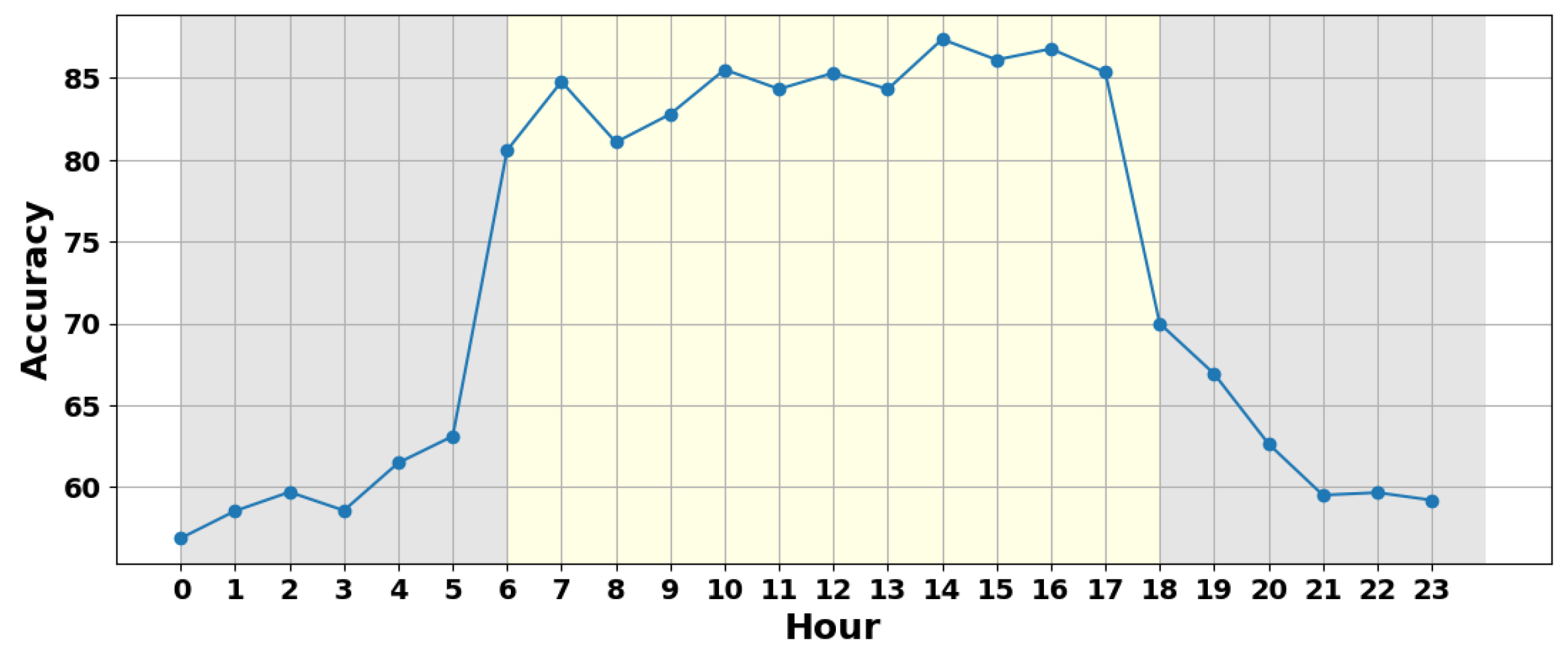
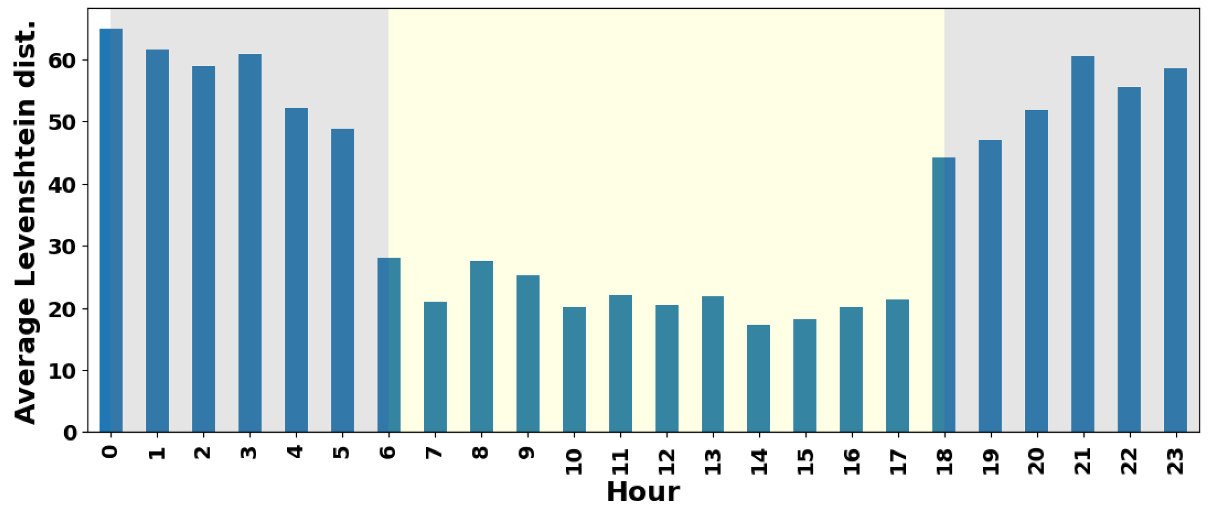
The analysis used the hour of image recording to evaluate the impact of operating conditions on system performance. As illustrated in Figure 29, recognition accuracy exhibits a marked dependence on time of day. Between 07:00 and 18:00, full-plate accuracy consistently exceeds 80 % , peaking at 87.4 % at 14:00. Outside these hours, accuracy drops significantly, reaching values below 60 % during late-night hours.
Figure 30 presents a complementary analysis based on Levenshtein distance. This figure shows that the average distance remains below 0.28 during daylight hours while increasing sharply during nighttime periods. The highest average distance occurs between 18:00 and 05:00, when ambient lighting is lowest, indicating a strong correlation between visibility and recognition fidelity.
The license plate recognition module demonstrated robust performance under favorable imaging conditions. Recognition quality was notably affected by environmental factors such as lighting and vehicle distance, particularly during low-light periods. These findings suggest that performance could be improved through sensor-level enhancements (e.g., infrared or auxiliary lighting) and adaptive preprocessing techniques to mitigate nighttime degradation.

4.3. Classifier Results

The training process used SVM with three kernel types: linear, RBF, and polynomial. These kernels were selected for their capacity to manage high-dimensional and nonlinear data, as typically found in processed point clouds. Also, the process scaled the geometric features using normalization techniques to maximize model performance, including minmax, maxabs, robust, and standard scaling. This preprocessing for standardizing variable ranges reduced the model’s sensitivity to outliers, improving training stability.
The evaluation tested the model using different BoW configurations by varying the number of generated visual words (5, 25, and 125) and the centroid initialization methods, which included random selection and K-means++. The implementation relied on the Mini-Batch K-means clustering algorithm. The evaluation uses multiple configurations to assess their impact on the classifier’s generalization ability.
Standard metrics such as macro F1-score and confusion matrices allow for the evaluation of the classifier’s performance. Table 9 shows that the configuration with the best results uses the RBF kernel in combination with the standard scaler. This configuration yielded overall macro F1-score rates exceeding 89 % .
Despite variations in the number of visual words and the centroid initialization methods, these parameters did not significantly impact the classifier’s overall performance. Moreover, comparative analysis revealed a substantial improvement in accuracy when geometric features and BoW representations were combined. As shown in the GFO (Geometric Features Only) and BWO (BoW Only) columns, the integration of both feature types enhanced the classifier’s precision and robustness, reinforcing its effectiveness for real-world deployment.
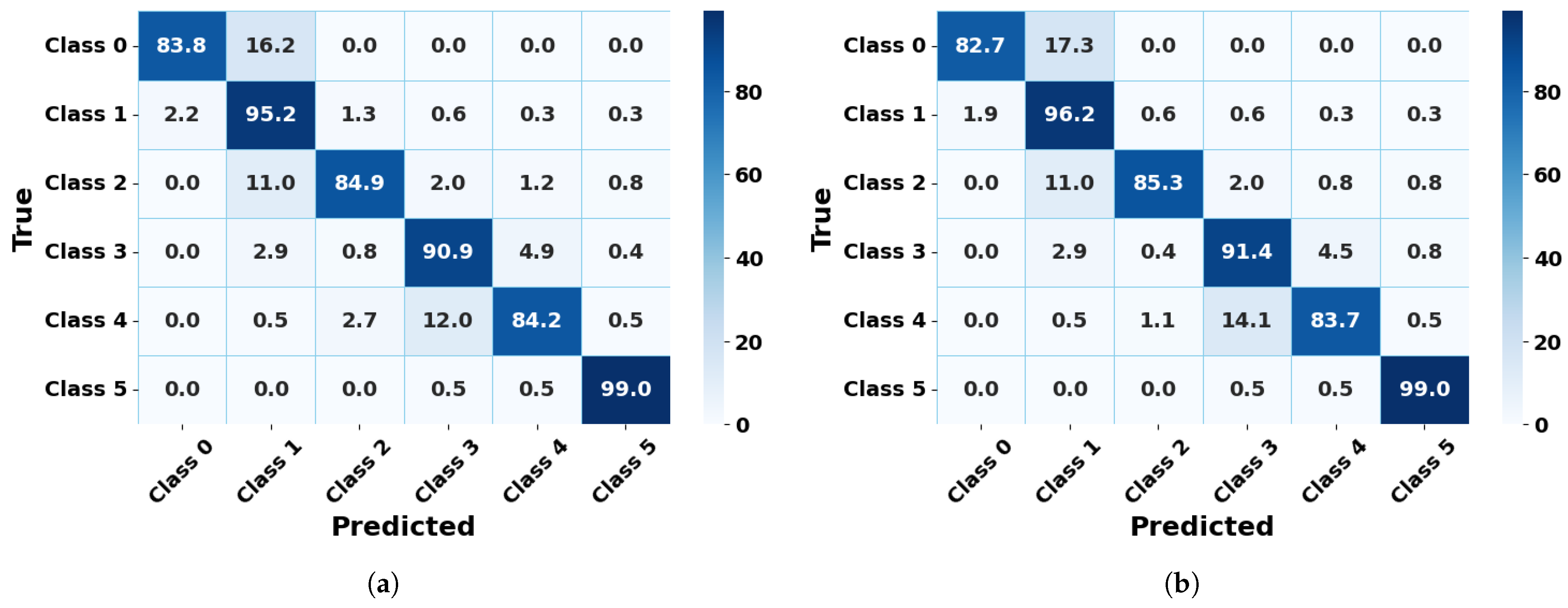
Figure 31 displays the confusion matrices generated during the validation phase of the highest-performing trained classifiers. These matrices provide a detailed overview of the system’s performance, highlighting the configurations that achieved the best results. Classifiers using the RBF kernel in combination with standard scaler demonstrated outstanding performance, with consistently high performance across all major vehicle classes. Among them, the classifier configured with an RBF kernel, standard scaler, random centroid initialization, and 25 visual words achieved the highest overall accuracy.
The classifier configuration with the best overall and per-class performance reached an overall accuracy of 89.9 % , a macro F1-score of 90.2 % , and a Matthews Correlation Coefficient (MCC) of 0.8795 , indicating strong class discrimination capability. Figure 32 shows the breakdown of precision, recall, and F1-score by class. Class 5 achieved the highest performance with an F1-score of 98.1 % , followed by classes 2 and 3, with F1-scores of 91.1 % and 89.0 % , respectively. Classes 0 and 1 exhibited greater variability between precision and recall: class 0 reached high precision ( 97.4 % ) but lower recall ( 82.7 % ), while class 1 showed the opposite pattern (precision of 78.4 % and recall of 96.2 % ), suggesting a tendency of the model to confuse these categories with adjacent ones. Overall, the graph highlights the classifier’s balanced behavior, validating its robustness and applicability in real-world vehicle classification scenarios.
Class-wise accuracy results were as follows: class 0— 82.7 % , class 1— 96.2 % , class 2— 85.3 % , class 3— 91.4 % , class 4— 83.7 % , and class 5— 99.0 % . The high performance of class 5, which includes vehicles with three or more axles, stands out, demonstrating the model’s ability to correctly identify complex vehicle configurations.
However, the confusion matrices revealed misclassification patterns, particularly between classes 3 and 4, and among categories 0, 1, and 2. These errors mainly stem from two factors. First, the visual similarity between certain vehicle types poses a considerable challenge. For example, minibuses with single rear wheels share geometric features with those with dual rear wheels, making them difficult to distinguish based solely on data captured by the laser sensor. Second, limitations in the laser sensor’s coverage also contributed to reduced accuracy in some categories. When vehicles travel too close to the lane divider, laser beams fail to fully capture the structure of the inner wheels, resulting in incomplete or distorted point clouds. This issue particularly affected classes where correct classification relies on the accurate detection of all vehicle axles.
The results confirm that using the RBF kernel in combination with the standard scaler optimizes classifier performance, even under challenging operational conditions. However, the confusion matrices reveal persistent misclassifications that highlight the need for further enhancements. These include integrating additional sensors to improve data capture in critical areas, such as rear dual-wheel detection, and refining the algorithms to better handle geometric similarities across classes. Implementing these improvements can mitigate the identified limitations and enhance the classifier’s ability to maintain high accuracy across a broader range of real-world operating scenarios.

4.4. Pilot Installation at a Toll Station

The SSICAV pilot installation was deployed at the Circasia toll station, operated by the Autopistas del Café concession, located in Filandia, Quindío. This toll plaza comprises five lanes with a standard width of 3.5 meters, separated by 2-meter-wide barriers. The site permitted the evaluation of the system’s performance under real operational conditions, with a high volume of vehicular flow and infrastructure representative of typical toll stations. The installation placed the system components on the central divider between lanes 2 and 3, counting from the left in the direction toward Pereira.
The system configuration included calibrating the ROI and filtering distance. Lane 2 was designated as the right lane, and Lane 3 as the left lane. For the right lane, it set the angular range between 30 ° and 30 ° , and for the left lane, between 150 ° and 210 ° , both with distance ranges of 1 to 3 meters from the LiDAR sensor. It sets the valid range for lateral filtering (Y-axis) in 1 to 3.5 meters, while the height (Z-axis) is from 1.5 to 3 meters. Figure 33 shows the final positioning of SSICAV’s sensors and devices.

5. Conclusions and Future Work

This work presented the design and implementation of an automatic vehicle counting and classification system (SSICAV) built on a multisensor architecture that integrates LiDAR technology, visible-spectrum cameras, and Doppler speed radars. The system was conceived with a modular and parameterizable design, enabling its adaptation to diverse operational contexts and facilitating scalability to more complex traffic scenarios.
Point cloud preprocessing represented a critical stage in the system pipeline. It involved distance-based filtering, RANSAC-based ground plane segmentation, angular correction, and statistical noise reduction. These procedures ensured a clean and accurate representation of the vehicle structure, enhancing the performance of downstream processing stages.
Vehicle characterization extracted geometric and structural descriptors, including surface normals and FPFH coded with a BoW model. A uniform sampling algorithm was applied to keypoint selection to reduce computational overhead while maintaining descriptive power. Additional geometric features such as vehicle length, height, and axle count were extracted and combined with visual words to train SVM classifiers. The resulting model achieved an overall accuracy of 89.9 % , with up to 99 % precision in complex vehicle classes (e.g., those with three or more axles), demonstrating its robustness under real-world conditions.
The axle-counting module achieved a 94.1 % accuracy for two-axle vehicles. However, performance declined in configurations that involve more axles due to occlusion caused by vehicles passing close to the median barrier. To expand the laser’s effective field of view, structural modifications, such as creating recessed channels or incorporating complementary sensors, are recommended to address this limitation.
The license plate recognition system achieved 79.94 % accuracy under optimal conditions but exhibited performance degradation during nighttime due to insufficient lighting and limited camera resolution. Enhancements, including infrared illumination, high-sensitivity cameras, and advanced character recognition algorithms, are proposed to ensure consistent performance across varying lighting conditions.
The proposed system is conceived as a modular architecture, designed to operate continuously in real traffic environments while meeting the functional requirements established by national road authorities. Its validation was carried out through field testing in an operational toll plaza, evaluating its classification accuracy, robustness under changing environmental conditions, and ability to integrate with existing traffic management systems. These results demonstrate the technical feasibility of implementing LiDAR and machine learning-based solutions for critical road infrastructure tasks in resource-constrained countries. They also lay the groundwork for future applications such as demand forecasting, maintenance planning, and the interoperability of ITS systems at the national level.
In future developments, we plan to explore the integration of our LiDAR-based system with heterogeneous data sources to enhance the analysis and understanding of traffic and mobility phenomena. The structured data produced by our system, including timestamps, vehicle categories, axle counts, and license plate information, could be combined with complementary data such as Floating Car Data (FCD), ALPR-based tracking, GPS probe data, or even Bluetooth/Wi-Fi sensor data. Such integration would support advanced applications such as traffic modeling, demand estimation, and mobility monitoring in real time.
This direction aligns with recent trends in transportation research that emphasize the fusion of heterogeneous data sources and the application of emerging ICTs to support intelligent transport system models. In particular, the integration of infrastructure-based observations with vehicle-generated data, such as Floating Car Data (FCD), has proven effective in improving traffic modeling and demand estimation, especially in situations with limited data availability. For instance, Ref. [109] explores the use of FCD and fixed sensors to estimate fundamental diagrams in the city of Santander, Spain, while Ref. [110] demonstrates how FCD alone can be used to estimate travel demand models despite the absence of traditional data sources. In this context, our LiDAR-based system could provide a reliable stream of structured vehicle-level data that complements these approaches, contributing to the calibration, validation, and enrichment of data-driven models in real-world applications.
In conclusion, the SSICAV has proven to be a robust, reliable, and high-performance system designed to transform vehicle management at toll plazas through advanced technologies. The identified challenges represent opportunities to optimize the system further and expand its applicability to more diverse operating scenarios. This work lays a solid foundation for the evolution of ITS, promoting their large-scale adoption in the future.
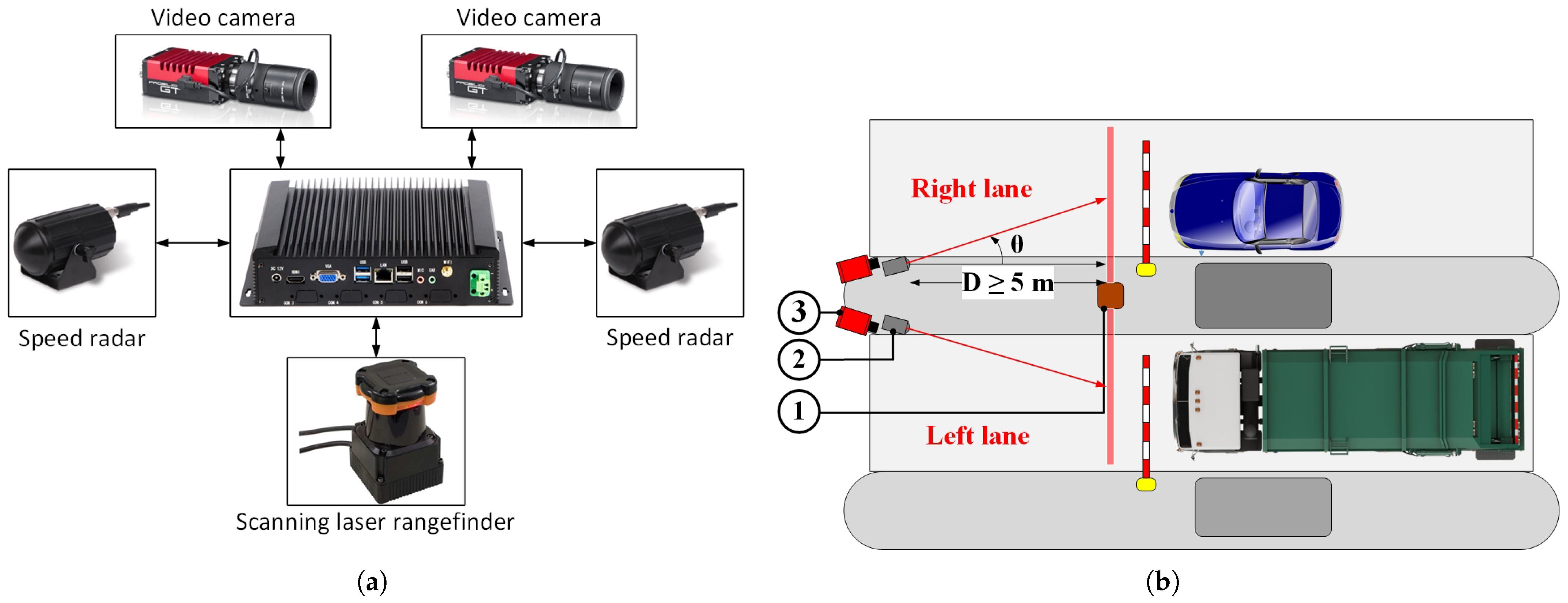
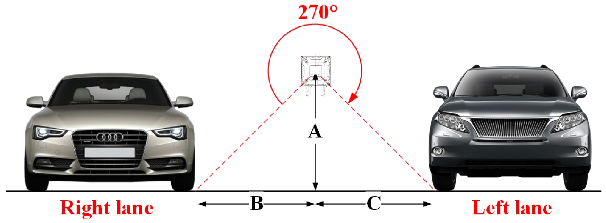
Author Contributions

Conceptualization, A.C.-R., E.F.C.-B. and B.B.-C.; methodology, A.C.-R., E.F.C.-B. and B.B.-C.; software, A.C.-R.; validation, A.C.-R.; formal analysis, A.C.-R.; investigation, A.C.-R., E.F.C.-B. and B.B.-C.; resources, A.C.-R.; data curation, A.C.-R.; writing—original draft preparation, A.C.-R.; writing—review and editing, A.C.-R., E.F.C.-B. and B.B.-C.; visualization, A.C.-R.; supervision, E.F.C.-B. and B.B.-C.; project administration, A.C.-R.; funding acquisition, A.C.-R. All authors have read and agreed to the published version of the manuscript.

Funding

This work is part of a beneficiary project from the National Doctorate in Business call number 758-2016, funded by the Ministry of Science, Technology and Innovation of Colombia, the Universidad del Valle, and the company SSI Soluciones y Suministros para Ingenierías SAS.

Institutional Review Board Statement

Not applicable.

Informed Consent Statement

Not applicable.

Data Availability Statement

The original data presented in the study are openly available in Zenodo at https://doi.org/10.5281/zenodo.10974361 (accessed on 22 May 2025).

Acknowledgments

We thank the Autopistas del Café concession for allowing us access to one of their toll stations to acquire the data presented in this work.

Conflicts of Interest

The authors declare no conflicts of interest.

Abbreviations

The following abbreviations are used in this manuscript:
ITSIntelligent transportation systems
LiDARLight detection and ranging
PCLPoint Cloud Library
RANSACRANdomized SAmple Consensus
SVMSupport vector machine
ROIRegion of interest
GUIGraphical User Interface
FPFHFast Point Feature Histograms
PFHPoint Feature Histogram
SPFHSimplified PFH
BoWBag-of-Words
INVIASInstituto Nacional de Vías
ANIAgencia Nacional de Infraestructura
CNNConvolutional Neural Networks
ALPRAutomatic License Plate Recognition
LBPLocal Binary Pattern

References

  1. Qi, L. Research on intelligent transportation system technologies and applications. In Proceedings of the 2008 Workshop on Power Electronics and Intelligent Transportation System, PEITS, Guangzhou, China, 2–3 August 2008; pp. 529–531. [Google Scholar] [CrossRef]
  2. Newman-Askins, R.; Ferreira, L.; Bunker, J. Intelligent transport systems evaluation: From theory to practice. In Proceedings of the 21st ARRB and 11th REAAA Conference, Cairns, VIC, Australia, 18–23 May 2003. [Google Scholar]
  3. Keerthi Kiran, V.; Parida, P.; Dash, S. Vehicle detection and classification: A review. In Proceedings of the 2019 Innovations in Bio-Inspired Computing and Applications, IBICA, Gunupur, Odisha, India, 16–18 December 2019; pp. 45–56. [Google Scholar] [CrossRef]
  4. Sundaravalli, G.; Krishnaveni, K. A survey on vehicle classification techniques. Int. J. Eng. Res. Comput. Sci. Eng. IJERCSE 2018, 5, 268–273. [Google Scholar]
  5. Celso, R.N.; Ting, Z.B.; Del Carmen, D.J.R.; Cajote, R.D. Two-Step Vehicle Classification System for Traffic Monitoring in the Philippines. In Proceedings of the 2018 IEEE Region 10 Annual International Conference, TENCON, Jeju, Republic of Korea, 28–31 October 2018; pp. 2028–2033. [Google Scholar] [CrossRef]
  6. Hussain, K.F.; Moussa, G.S. Automatic Vehicle Classification System using range sensor. In Proceedings of the 2005 International Conference on Information Technology: Coding and Computing, ITCC, Las Vegas, NV, USA, 4–6 April 2005; Volume 2, pp. 107–112. [Google Scholar] [CrossRef]
  7. Singh, V.; Srivastava, A.; Kumar, S.; Ghosh, R. A Structural Feature Based Automatic Vehicle Classification System at Toll Plaza. In Proceedings of the 2019 4th International Conference on Internet of Things and Connected Technologies (ICIoTCT), Jaipur, India, 9–10 May 2019; Volume 1122, pp. 1–10. [Google Scholar] [CrossRef]
  8. Lopes, J.; Bento, J.; Huang, E.; Antoniou, C.; Ben-Akiva, M. Traffic and mobility data collection for real-time applications. In Proceedings of the 13th International IEEE Conference on Intelligent Transportation Systems, Funchal, Portugal, 19–22 September 2010; pp. 216–223. [Google Scholar] [CrossRef]
  9. Gordon, R.L.; Tighe, W. Traffic Control Systems Handbook; Technical Report FHWA-HOP-06-006; Office of Transportation Management, Federal Highway Administration: Washington, DC, USA, 2005.
  10. Cheung, S.Y.; Varaiya, P. Traffic Surveillance by Wireless Sensor Networks: Final Report; Technical Report UCB-ITS-PRR-2007-4; California Path Program, Institute of Transportation Studies, University of California: Berkeley, CA, USA, 2007. [Google Scholar]
  11. Nkaro, A. Traffic Data Collection and Analysis; Technical Report; Roads Department, Ministry of Works and Transport: Gaborone, Botsuana, 2004.
  12. Shekade, A.; Mahale, R.; Shetage, R.; Singh, A.; Gadakh, P. Vehicle Classification in Traffic Surveillance System using YOLOv3 Model. In Proceedings of the 2020 International Conference on Electronics and Sustainable Communication Systems (ICESC), Coimbatore, India, 2–4 July 2020; pp. 1015–1019. [Google Scholar] [CrossRef]
  13. Shin, J.; Koo, B.; Kim, Y.; Paik, J. Deep binary classification via multi-resolution network and stochastic orthogonality for subcompact vehicle recognition. Sensors 2020, 20, 2715. [Google Scholar] [CrossRef]
  14. Wang, K.; Liu, Y. Vehicle Classification System Based on Dynamic Bayesian Network. In Proceedings of the 2014 IEEE International Conference on Service Operations and Logistics, and Informatics, Qingdao, China, 8–10 October 2014; pp. 22–26. [Google Scholar] [CrossRef]
  15. Hasnat, A.; Shvai, N.; Meicler, A.; Maarek, P.; Nakib, A. New vehicle classification method based on hybrid classifiers. In Proceedings of the 2018 25th IEEE International Conference on Image Processing (ICIP), Athens, Greece, 7–10 October 2018; pp. 3084–3088. [Google Scholar] [CrossRef]
  16. Sandhawalia, H.; Rodriguez-Serrano, J.A.; Poirier, H.; Csurka, G. Vehicle type classification from laser scanner profiles: A benchmark of feature descriptors. In Proceedings of the 2013 IEEE Conference on Intelligent Transportation Systems, ITSC, The Hague, The Netherlands, 6–9 October 2013; pp. 517–522. [Google Scholar] [CrossRef]
  17. Ripoll, N.G.; Aguilera, L.E.G.; Belenguer, F.M.; Salcedo, A.M.; Merelo, F.J.B. Design, implementation, and configuration of laser systems for vehicle detection and classification in real time. Sensors 2021, 21, 2082. [Google Scholar] [CrossRef]
  18. Zheng, J.; Yang, S.; Wang, X.; Xia, X.; Xiao, Y.; Li, T. A Decision Tree Based Road Recognition Approach Using Roadside Fixed 3D LiDAR Sensors. IEEE Access 2019, 7, 53878–53890. [Google Scholar] [CrossRef]
  19. Ye, Z.; Wang, Z.; Chen, X.; Zhou, T.; Yu, C.; Guo, J.; Li, J. ZPVehicles: A dataset of large vehicle 3D point cloud data. In Proceedings of the 2023 IEEE International Workshop on Metrology for Automotive, MetroAutomotive, Modena, Italy, 28–30 June 2023; pp. 234–239. [Google Scholar] [CrossRef]
  20. Caesar, H.; Bankiti, V.; Lang, A.H.; Vora, S.; Liong, V.E.; Xu, Q.; Krishnan, A.; Pan, Y.; Baldan, G.; Beijbom, O. Nuscenes: A multimodal dataset for autonomous driving. In Proceedings of the 2020 IEEE Computer Society Conference on Computer Vision and Pattern Recognition, Seattle, WA, USA, 13–19 June 2020; pp. 11618–11628. [Google Scholar] [CrossRef]
  21. Xiao, P.; Shao, Z.; Hao, S.; Zhang, Z.; Chai, X.; Jiao, J.; Li, Z.; Wu, J.; Sun, K.; Jiang, K.; et al. PandaSet: Advanced Sensor Suite Dataset for Autonomous Driving. In Proceedings of the 2021 IEEE Conference on Intelligent Transportation Systems, ITSC, Indianapolis, IN, USA, 19–22 September 2021; pp. 3095–3101. [Google Scholar] [CrossRef]
  22. Schumann, O.; Hahn, M.; Scheiner, N.; Weishaupt, F.; Tilly, J.F.; Dickmann, J.; Wohler, C. RadarScenes: A Real-World Radar Point Cloud Data Set for Automotive Applications. In Proceedings of the 2021 IEEE 24th International Conference on Information Fusion, FUSION, Sun City, South Africa, 1–4 November 2021. [Google Scholar] [CrossRef]
  23. Kim, K.; Kim, C.; Jang, C.; Sunwoo, M.; Jo, K. Deep learning-based dynamic object classification using LiDAR point cloud augmented by layer-based accumulation for intelligent vehicles. Expert Syst. Appl. 2021, 2021, 113861. [Google Scholar] [CrossRef]
  24. Unnikrishnan, R. Statistical Approaches to Multi-scale Point Cloud Processing. Ph.D. Thesis, The Robotics Institute, Carnegie Mellon University, Pittsburgh, PA, USA, 2008. [Google Scholar]
  25. Yu, S.; Wang, M.; Zhang, C.; Li, J.; Yan, K.; Liang, Z.; Wei, R. A Dynamic Multi-Branch Neural Network Module for 3D Point Cloud Classification and Segmentation Using Structural Re-parametertization. In Proceedings of the 2023 11th International Conference on Agro-Geoinformatics, Agro-Geoinformatics, Wuhan, China, 25–28 July 2023; pp. 1–6. [Google Scholar] [CrossRef]
  26. Rusu, R.B. Semantic 3D Object Maps for Everyday Manipulation in Human Living Environments. Ph.D. Thesis, Institute of Computer Science, Technical University of Munich, Munich, Germany, 2009. [Google Scholar] [CrossRef]
  27. Fischler, M.A.; Bolles, R.C. Random sample consensus: A Paradigm for Model Fitting with Applications to Image Analysis and Automated Cartography. Commun. ACM 1981, 24, 381–395. [Google Scholar] [CrossRef]
  28. Csurka, G.; Dance, C.R.; Fan, L.; Willamowski, J.; Bray, C. Visual Categorization with Bags of Keypoints. In Proceedings of the ECCV European Conference on Computer Vision, Workshop on Statistical Learning in Computer Vision, Prague, Czech Republic, 15 May 2004. [Google Scholar]
  29. Sivic, J.; Russell, B.; Efros, A.; Zisserman, A.; Freeman, B. Discovering objects and their location. In Proceedings of the Tenth IEEE International Conference on Computer Vision (ICCV’05) Volume 1, Beijing, China, 17–21 October 2005; pp. 370–377. [Google Scholar]
  30. Li, X.; Godil, A.; Wagan, A. Spatially enhanced bags of words for 3D shape retrieval. In Advances in Visual Computing; Lecture Notes in Computer Science; Lecture Notes in Artificial Intelligence and Lecture Notes in Bioinformatics; Springer: Berlin/Heidelberg, Germany, 2008; Volume 5358 LNCS, pp. 349–358. [Google Scholar] [CrossRef]
  31. Zhan, Q.; Yu, L. Objects classification from laser scanning data based on multi-class support vector machine. In Proceedings of the 2011 International Conference on Remote Sensing, Environment and Transportation Engineering, RSETE, Nanjing, China, 24–26 June 2011; pp. 520–523. [Google Scholar] [CrossRef]
  32. Raktrakulthum, P.A.; Netramai, C. Vehicle classification in congested traffic based on 3D point cloud using SVM and KNN. In Proceedings of the 2017 9th International Conference on Information Technology and Electrical Engineering, ICITEE, Phuket, Thailand, 12–13 October 2017; pp. 1–6. [Google Scholar] [CrossRef]
  33. Wei, S. Three-dimensional point cloud classification based on multi-scale dynamic graph convolutional network. In Proceedings of the 2021 3rd International Academic Exchange Conference on Science and Technology Innovation, IAECST, Guangzhou, China, 10–12 December 2021; pp. 603–606. [Google Scholar] [CrossRef]
  34. Zhang, Z.; Wang, Q.; Wang, M.; Shen, T. Graph Neural Network with Multi-Kernel Learning for Multispectral Point Cloud Classification. In Proceedings of the 2023 International Geoscience and Remote Sensing Symposium (IGARSS), Pasadena, CA, USA, 16–21 July 2023; pp. 970–973. [Google Scholar] [CrossRef]
  35. Kang, Z.; Yang, J.; Zhong, R. A Bayesian-Network-Based Classification Method Integrating Airborne LiDAR Data with Optical Images. IEEE J. Sel. Top. Appl. Earth Obs. Remote Sens. 2017, 10, 1651–1661. [Google Scholar] [CrossRef]
  36. Colombia. Ministry of Transportation. Instituto Nacional de Vías INVIAS. Available online: https://www.invias.gov.co (accessed on 22 May 2025).
  37. Colombia. Ministry of Transportation. Agencia Nacional de Infraestructura, ANI. Available online: https://www.ani.gov.co (accessed on 22 May 2025).
  38. Jeng, S.T.; Ritchie, S.G. Real-time vehicle classification using inductive loop signature data. Transp. Res. Rec. 2008, 2086, 8–22. [Google Scholar] [CrossRef]
  39. Coifman, B.; Kim, S.B. Speed estimation and length based vehicle classification from freeway single-loop detectors. Transp. Res. Part C Emerg. Technol. 2009, 17, 349–364. [Google Scholar] [CrossRef]
  40. Wu, L.; Coifman, B. Improved vehicle classification from dual-loop detectors in congested traffic. Transp. Res. Part C Emerg. Technol. 2014, 46, 222–234. [Google Scholar] [CrossRef]
  41. Rajab, S.A.; Mayeli, A.; Refai, H.H. Vehicle classification and accurate speed calculation using multi-element piezoelectric sensor. In Proceedings of the 2014 IEEE Intelligent Vehicles Symposium Proceedings, Dearborn, MI, USA, 8–11 June 2014; pp. 894–899. [Google Scholar] [CrossRef]
  42. Premaratne, P.; Jawad Kadhim, I.; Blacklidge, R.; Lee, M. Comprehensive review on vehicle Detection, classification and counting on highways. Neurocomputing 2023, 556, 126627. [Google Scholar] [CrossRef]
  43. Lin, C.J.; Jeng, S.Y.; Lioa, H.W. A Real-Time Vehicle Counting, Speed Estimation, and Classification System Based on Virtual Detection Zone and YOLO. Math. Probl. Eng. 2021, 2021, 1577614. [Google Scholar] [CrossRef]
  44. Patanè, M.; Fusiello, A. Vehicle classification from profile measures. In Proceedings of the 2020 25th International Conference on Pattern Recognition (ICPR), Milan, Italy, 10–15 January 2020; pp. 6656–6663. [Google Scholar] [CrossRef]
  45. Ruan, G.; Hu, T.; Ding, C.; Yang, K.; Kong, F.; Cheng, J.; Yan, R. Fine-grained vehicle recognition under low light conditions using EfficientNet and image enhancement on LiDAR point cloud data. Sci. Rep. 2025, 15, 1–13. [Google Scholar] [CrossRef] [PubMed]
  46. Abdelbaki, H.M.; Hussain, K.; Gelenbe, E. A laser intensity image based automatic vehicle classification system. In Proceedings of the 2001 IEEE Intelligent Transportation Systems, ITSC, Oakland, CA, USA, 25–29 August 2001; pp. 460–465. [Google Scholar] [CrossRef]
  47. Gomez, A.; Hernandez, P.; Bladimir, B.C. Vehicle Classification Based on a Bag of Visual Words and Range Images Usage. Ing. Compet. 2015, 17, 49–61. [Google Scholar]
  48. Sato, T.; Aoki, Y.; Takebayashi, Y. Vehicle axle counting using two LIDARs for toll collection systems. In Proceedings of the 2014 21st World Congress on Intelligent Transport Systems, ITSWC: Reinventing Transportation in Our Connected World, Detroit, MI, USA, 7–11 September 2014. [Google Scholar]
  49. Mogelmose, A.; Moeslund, T.B. Analyzing Wheels of Vehicles in Motion Using Laser Scanning. In Proceedings of the IEEE Computer Society Conference on Computer Vision and Pattern Recognition Workshops, Las Vegas, NV, USA, 26 June–1 July 2016; pp. 1601–1608. [Google Scholar] [CrossRef]
  50. Xu, Z.; Wei, J.; Chen, X. Vehicle recognition and classification method based on laser scanning point cloud data. In Proceedings of the 2015 3rd International Conference on Transportation Information and Safety, ICTIS, Wuhan, China, 25–28 June 2015; pp. 44–49. [Google Scholar] [CrossRef]
  51. Geiger, A.; Lenz, P.; Stiller, C.; Urtasun, R. Vision meets robotics: The KITTI dataset. Int. J. Robot. Res. 2013, 32, 1231–1237. [Google Scholar] [CrossRef]
  52. Hokuyo. Scanning Rangefinder UTM-30LX. Hokuyo Automatic Co. Ltd. Available online: https://www.hokuyo-aut.jp/search/single.php?serial=169 (accessed on 22 May 2025).
  53. Stalker. Stalker Stationary Speed Sensor. Applied Concepts Inc. Available online: https://stalkersensors.com/speed-sensors/stationary-speed-sensor (accessed on 22 May 2025).
  54. Allied Vision. Prosilica GT 1290. Available online: https://www.alliedvision.com/en/camera-selector/detail/prosilica-gt/1290 (accessed on 22 May 2025).
  55. Campo-Ramírez, A.; Caicedo-Bravo, E.F.; Bacca-Cortes, E.B. A Point Cloud Dataset of Vehicles Passing through a Toll Station for Use in Training Classification Algorithms. Data 2024, 9, 87. [Google Scholar] [CrossRef]
  56. Rusu, R.B.; Cousins, S. 3D is here: Point Cloud Library (PCL). In Proceedings of the 2011 IEEE International Conference on Robotics and Automation, Shanghai, China, 9–13 May 2011; pp. 1–4. [Google Scholar] [CrossRef]
  57. Biggs, G. Hokuyoaist: Hokuyo Range Sensor Driver. Available online: https://github.com/gbiggs/hokuyoaist (accessed on 22 May 2025).
  58. Biggs, G. HokuyoAIST Range Sensor Driver — HokuyoAIST 3.0.0 Documentation. Available online: https://gbiggs.github.io/hokuyoaist (accessed on 22 May 2025).
  59. Liechti, C. pySerial. Available online: https://pypi.org/project/pyserial (accessed on 22 May 2025).
  60. Allied Vision. Vimba. Available online: https://www.alliedvision.com/en/products/vimba-sdk (accessed on 22 May 2025).
  61. Duckworth, D. Pykalman. Available online: https://pypi.org/project/pykalman (accessed on 22 May 2025).
  62. Movellan, J.R. Discrete Time Kalman Filters and Smoothers. Available online: https://mplab.ucsd.edu/tutorials/Kalman.pdf (accessed on 22 May 2025).
  63. Miller, J.W. Kalman Filter and Smoother. Available online: https://jwmi.github.io/ASM/6-KalmanFilter.pdf (accessed on 22 May 2025).
  64. Reid, I.; Term, H. Estimation II. Available online: https://www.robots.ox.ac.uk/~ian/Teaching/Estimation/LectureNotes2.pdf (accessed on 22 May 2025).
  65. Rusu, R.B.; Blodow, N.; Marton, Z.; Soos, A.; Beetz, M. Towards 3D object maps for autonomous household robots. In Proceedings of the 2007 IEEE International Conference on Intelligent Robots and Systems, San Diego, CA, USA, 29 October–2 November 2007; pp. 3191–3198. [Google Scholar] [CrossRef]
  66. Hinterstoisser, S.; Cagniart, C.; Ilic, S.; Sturm, P.; Navab, N.; Fua, P.; Lepetit, V. Gradient response maps for real-time detection of textureless objects. IEEE Trans. Pattern Anal. Mach. Intell. 2012, 34, 876–888. [Google Scholar] [CrossRef]
  67. Hoppe, H.; DeRose, T.; Duchamp, T.; McDonald, J.; Stuetzle, W. Surface reconstruction from unorganized points. Comput. Graph. ACM 1992, 26, 71–78. [Google Scholar] [CrossRef]
  68. Zheng, D.H.; Xu, J.; Chen, R.X. Generation method of normal vector from disordered point cloud. In Proceedings of the 2009 Joint Urban Remote Sensing Event, Shanghai, China, 20–22 May 2009; pp. 17–21. [Google Scholar] [CrossRef]
  69. Rusu, R.B.; Blodow, N.; Marton, Z.C.; Beetz, M. Aligning point cloud views using persistent feature histograms. In Proceedings of the 2008 IEEE/RSJ International Conference on Intelligent Robots and Systems, IROS, Nice, France, 22–26 September 2008; pp. 3384–3391. [Google Scholar] [CrossRef]
  70. Lalonde, J.F.; Unnikrishnan, R.; Vandapel, N.; Hebert, M. Scale selection for classification of point-sampled 3D surfaces. In Proceedings of the Fifth International Conference on 3-D Digital Imaging and Modeling (3DIM’05), Ottawa, ON, Canada, 13–16 June 2005; pp. 285–292. [Google Scholar] [CrossRef]
  71. Mitra, N.J.; Nguyen, A. Estimating Surface Normals in Noisy Point Cloud Data. In Proceedings of the Proceedings of the Nineteenth Annual Symposium on Computational Geometry, San Diego, CA, USA, 8–10 June 2003; pp. 322–328. [Google Scholar] [CrossRef]
  72. García García, A. Towards a real-time 3D object recognition pipeline on mobile GPGPU computing platforms using low-cost RGB-D sensors. Ph.D. Thesis, Department of Computer Technology (DTIC), University of Alicante, Alicante, España, 2015. [Google Scholar]
  73. Zhou, R.; Li, X.; Jiang, W. 3D Surface Matching by a Voxel-Based Buffer-Weighted Binary Descriptor. IEEE Access 2019, 7, 86635–86650. [Google Scholar] [CrossRef]
  74. Sipiran, I.; Bustos, B. Harris 3D: A robust extension of the Harris operator for interest point detection on 3D meshes. Vis. Comput. 2011, 27, 963–976. [Google Scholar] [CrossRef]
  75. Flint, A.; Dick, A.; Van Den Hengel, A. Thrift: Local 3D structure recognition. In Proceedings of the Digital Image Computing Techniques and Applications: 9th Biennial Conference of the Australian Pattern Recognition Society, DICTA 2007, Glenelg, SA, Australia, 3–5 December 2007; pp. 182–188. [Google Scholar] [CrossRef]
  76. Steder, B.; Rusu, R.B.; Konolige, K.; Burgard, W. Point feature extraction on 3D range scans taking into account object boundaries. In Proceedings of the 2011 IEEE International Conference on Robotics and Automation, Shanghai, China, 9–13 May 2011; pp. 2601–2608. [Google Scholar] [CrossRef]
  77. Yu, Z. Intrinsic shape signatures: A shape descriptor for 3D object recognition. In Proceedings of the 2009 IEEE 12th International Conference on Computer Vision Workshops, ICCV Workshops, Kyoto, Japan, 27 September–4 October 2009; pp. 689–696. [Google Scholar] [CrossRef]
  78. Rusu, R.B.; Blodow, N.; Beetz, M. Fast Point Feature Histograms (FPFH) for 3D Registration. In Proceedings of the IEEE International Conference on Robotics and Automation, Kobe, Japan, 12–17 May 2009; pp. 3212–3217. [Google Scholar] [CrossRef]
  79. Rusu, R.B.; Marton, Z.C.; Blodow, N.; Beetz, M. Learning informative point classes for the acquisition of object model maps. In Proceedings of the 2008 10th International Conference on Control, Automation, Robotics and Vision, ICARCV 2008, Hanoi, Vietnam, 17–20 December 2008; pp. 643–650. [Google Scholar] [CrossRef]
  80. Wahl, E.; Hillenbrand, U.; Hirzinger, G. Surflet-pair-relation histograms: A statistical 3D-shape representation for rapid classification. In Proceedings of the Fourth International Conference on 3-D Digital Imaging and Modeling, 2003. 3DIM, Banff, AB, Canada, 6–10 October 2003; pp. 474–481. [Google Scholar] [CrossRef]
  81. Garstka, J.; Peters, G. Evaluation of local 3-D point cloud descriptors in terms of suitability for object classification. In Proceedings of the 13th International Conference on Informatics in Control, Automation and Robotics—Volume 2: ICINCO, Lisbon, Portugal, 29–31 July 2016; Volume 2, pp. 540–547. [Google Scholar] [CrossRef]
  82. Sudderth, E.B.; Torralba, A.; Freeman, W.T.; Willsky, A.S. Learning hierarchical models of scenes, objects, and parts. In Proceedings of the Tenth IEEE International Conference on Computer Vision (ICCV’05) Volume 1, Beijing, China, 17–21 October 2005; pp. 1331–1338. [Google Scholar] [CrossRef]
  83. Martínez-Gómez, J.; Morell, V.; Cazorla, M.; García-Varea, I. Semantic localization in the PCL library. Robot. Auton. Syst. 2016, 75, 641–648. [Google Scholar] [CrossRef]
  84. Madry, M.; Ek, C.H.; Detry, R.; Hang, K.; Kragic, D. Improving generalization for 3D object categorization with Global Structure Histograms. In Proceedings of the IEEE International Conference on Intelligent Robots and Systems, Vilamoura-Algarve, Portugal, 7–12 October 2012; pp. 1379–1386. [Google Scholar] [CrossRef]
  85. Garstka, J.; Peters, G. Self-learning 3D object classification. In Proceedings of the 7th International Conference on Pattern Recognition Applications and Methods ICPRAM, Funchal, Madeira, Portugal, 16–18 January 2018; pp. 511–519. [Google Scholar] [CrossRef]
  86. Toldo, R.; Castellani, U.; Fusiello, A. The Bag of Words approach for retrieval and categorization of 3D objects. Vis. Comput. 2010, 26, 1257–1269. [Google Scholar] [CrossRef]
  87. Liu, M.; Li, X.; Dezert, J.; Luo, C. Generic object recognition based on the fusion of 2D and 3D SIFT descriptors. In Proceedings of the 2015 18th International Conference on Information Fusion, Fusion 2015, Washington, DC, USA, 6–9 July 2015; pp. 1085–1092. [Google Scholar]
  88. Toldo, R.; Castellani, U.; Fusiello, A. A Bag of Words Approach for 3d Object Categorization; Lecture Notes in Computer Science; Lecture Notes in Artificial Intelligence and Lecture Notes in Bioinformatics; Springer: Berlin/Heidelberg, Germany, 2009; Volume 5496 LNCS, pp. 116–127. [Google Scholar] [CrossRef]
  89. Béjar Alonso, J. K-means vs Mini Batch K-Means: A Comparison; Technical Report; Departament de Llenguatges i Sistemes Informàtics, Universitat Politècnica de Catalunya: Barcelona, Spain, 2013. [Google Scholar]
  90. Pedregosa, F.; Varoquaux, G.; Gramfort, A.; Michel, V.; Thirion, B.; Grisel, O.; Blondel, M.; Prettenhofer, P.; Weiss, R.; Dubourg, V.; et al. Scikit-learn: Machine Learning in Python. J. Mach. Learn. Res. 2011, 12, 2825–2830. [Google Scholar]
  91. Gallego Ripoll, N. Requisitos técnicos para la aplicación de sensores de tecnología láser en sistemas inteligentes de transporte (ITS). Ph.D. Thesis, Departamento de Ingeniería Electrónica, Universidad Politécnica de Valencia, Valencia, España, 2010. [Google Scholar]
  92. Alshaher, H. Studying the Effects of Feature Scaling in Machine Learning. Ph.D. Thesis, Computer Science, North Carolina Agricultural and Technical State University, Greensboro, NC, Australia, 2021. [Google Scholar]
  93. Wang, L.; Kou, Q.; Wei, R.; Zhou, L.; Fang, T.; Zhang, J. An Improved Substation Equipment Recognition Algorithm by KNN Classification of Subspace Feature Vector. In Proceedings of the 2021 China Automation Congress, CAC, Beijing, China, 22–24 October 2021; pp. 7541–7546. [Google Scholar] [CrossRef]
  94. Chang, C.C.; Lin, C.J. LIBSVM: A Library for support vector machines. ACM Trans. Intell. Syst. Technol. 2011, 2, 1–40. [Google Scholar] [CrossRef]
  95. Platt, J.C. Probabilistic Outputs for Support Vector Machines and Comparisons to Regularized Likelihood Methods. Adv. Large Margin Classif. 1999, 10, 61–74. [Google Scholar]
  96. Xu, J. An extended one-versus-rest support vector machine for multi-label classification. Neurocomputing 2011, 74, 3114–3124. [Google Scholar] [CrossRef]
  97. Nguyen, T.T.; Nguyen, T.T. A real time license plate detection system based on boosting learning algorithm. In Proceedings of the 2012 5th International Congress on Image and Signal Processing (CISP 2012), Chongqing, China, 16–18 October 2012; pp. 819–823. [Google Scholar] [CrossRef]
  98. Dlagnekov, L. License Plate Detection Using Adaboost; Technical Report; Computer Science and Engineering Department, University of California San Diego: San Diego, CA, USA, 2004. [Google Scholar]
  99. Ojala, T.; Pietikhenl, M.; Harwood, D. Performance evaluation of texture measures with classification based on Kullback discrimination of distributions. In Proceedings of the 12th International Conference on Pattern Recognition, Jerusalem, Israel, 9–13 October 1994; pp. 582–585. [Google Scholar]
  100. Freund, Y.; Schapire, R. A decision theoretic generalisation of online learning. Comput. Syst. Sci. 1997, 55, 119–139. [Google Scholar] [CrossRef]
  101. Viola, P.; Jones, M. Rapid object detection using a boosted cascade of simple features. In Proceedings of the IEEE Computer Society Conference on Computer Vision and Pattern Recognition, Kauai, HI, USA, 8–14 December 2001; Volume 1. [Google Scholar] [CrossRef]
  102. Jain, P.H.; Kumar, V.; Samuel, J.; Singh, S.; Mannepalli, A.; Anderson, R. Artificially Intelligent Readers: An Adaptive Framework for Original Handwritten Numerical Digits Recognition with OCR Methods. Information 2023, 14, 305. [Google Scholar] [CrossRef]
  103. Rai, R.; Shitole, S.; Sutar, P.; Kaldhone, S.; Jadhav, P.J.D. Automatic License Plate Recognition Using Yolov4 and Tesseract Ocr. Int. J. Innov. Res. Comput. Commun. Eng. 2022, 10, 58–67. [Google Scholar] [CrossRef]
  104. Ayvacı, A.; Tümer, A.E. Deep Learning Method for Handwriting Recognition. MANAS J. Eng. 2021, 9, 85–92. [Google Scholar] [CrossRef]
  105. Shambharkar, Y.; Salagrama, S.; Sharma, K.; Mishra, O.; Parashar, D. An Automatic Framework for Number Plate Detection using OCR and Deep Learning Approach. Int. J. Adv. Comput. Sci. Appl. 2023, 14, 8–14. [Google Scholar] [CrossRef]
  106. Agrawal, A.K.; Shrivas, A.K.; Awasthi, V.K. A robust model for handwritten digit recognition using machine and deep learning technique. In Proceedings of the 2021 2nd International Conference for Emerging Technology, INCET 2021, Belgaum, India, 21–23 May 2021; pp. 1–4. [Google Scholar] [CrossRef]
  107. Raquib, M.; Hossain, M.A.; Islam, M.K.; Miah, M.S. VashaNet: An automated system for recognizing handwritten Bangla basic characters using deep convolutional neural network. Mach. Learn. Appl. 2024, 17, 100568. [Google Scholar] [CrossRef]
  108. Soghadi, Z.T. License Plate Detection and Recognition by Convolutional Neural Networks. Master’s Thesis, Concordia University, Montreal, QC, Canada, 2020. [Google Scholar] [CrossRef]
  109. Alonso, B.; Musolino, G.; Rindone, C.; Vitetta, A. Estimation of a Fundamental Diagram with Heterogeneous Data Sources: Experimentation in the City of Santander. ISPRS Int. J. Geo-Inf. 2023, 12, 418. [Google Scholar] [CrossRef]
  110. Croce, A.I.; Musolino, G.; Rindone, C.; Vitetta, A. Estimation of travel demand models with limited information: Floating car data for parameters’ calibration. Sustainability 2021, 13, 8838. [Google Scholar] [CrossRef]
Figure 1. (a) Connection diagram of the vehicle counting and classification system. (b) Spatial arrangement of sensors at a toll station for two adjacent lanes. (1) Scanning laser rangefinder. (2) Speed radars. (3) Video cameras [55].
Futuretransp 05 00105 g001
Figure 2. Spatial arrangement of the scanning laser rangefinder [55].
Futuretransp 05 00105 g002
Figure 3. Physical structure of the vehicle counting and classification system.
Futuretransp 05 00105 g003
Figure 4. General block diagram of the vehicle counting and classification system software.
Futuretransp 05 00105 g004
Figure 5. Configuration and processing interface: operation screen.
Futuretransp 05 00105 g005
Figure 6. Block diagram of the data acquisition module.
Futuretransp 05 00105 g006
Figure 7. Region of interest (ROI) of valid sample selection [55].
Futuretransp 05 00105 g007
Figure 8. Angular range of the laser rangefinder [55].
Futuretransp 05 00105 g008
Figure 9. (a) Speed smoothing using Kalman filtering and smoothing. (b) Three-dimensional image of a raw point cloud [55].
Futuretransp 05 00105 g009
Figure 10. Block diagram of the point cloud preprocessing module.
Futuretransp 05 00105 g010
Figure 11. (a) Distance filtering region [55]. (b) Point cloud with distance filtering [55].
Futuretransp 05 00105 g011
Figure 12. Point cloud with ground surface extraction [55].
Futuretransp 05 00105 g012
Figure 13. Point cloud with statistical filtering [55].
Futuretransp 05 00105 g013
Figure 14. Block diagram of the feature extraction module.
Futuretransp 05 00105 g014
Figure 15. Graphical representation of the Darboux reference frame.
Futuretransp 05 00105 g015
Figure 16. (a) Point cloud with five random points highlighted to illustrate the FPFH. (b) FPFH for the five random points in the point cloud.
Futuretransp 05 00105 g016
Figure 17. (a) Point cloud with the keypoints assigned to each visual word differentiated with colors. (b) BoW for the point cloud.
Futuretransp 05 00105 g017
Figure 18. Geometric features of the vehicle in the point cloud [55].
Futuretransp 05 00105 g018
Figure 19. Region of the tires in contact with the ground.
Futuretransp 05 00105 g019
Figure 20. Clusters identified as vehicle axles.
Futuretransp 05 00105 g020
Figure 21. Example of visualization of the LBP matrix.
Futuretransp 05 00105 g021
Figure 22. (a) Cascade classifier structure. (b) Results of some stages of the cascade classifier.
Futuretransp 05 00105 g022
Figure 23. CNN model architecture for license plate character recognition.
Futuretransp 05 00105 g023
Figure 24. Character recognition results.
Futuretransp 05 00105 g024
Figure 25. Block diagram of the multi-frame license plate recognition process.
Futuretransp 05 00105 g025
Figure 26. Confusion matrix for axle classification (absolute values).
Futuretransp 05 00105 g026
Figure 27. Normalized confusion matrix for axle classification (percentage).
Futuretransp 05 00105 g027
Figure 28. Precision, recall, and F1-score by axle class.
Futuretransp 05 00105 g028
Figure 29. Full-plate recognition accuracy per hour.
Futuretransp 05 00105 g029
Figure 30. Average normalized Levenshtein distance by hour.
Futuretransp 05 00105 g030
Figure 31. Validation result of the classifier configured with standard scaler, RBF kernel, and random centroid initialization: (a) 5 visual words. (b) 25 visual words.
Futuretransp 05 00105 g031
Figure 32. Per-Class precision, recall, and F1-score for the best classifier configuration.
Futuretransp 05 00105 g032
Figure 33. Installed sensors at the toll station: (a) Laser. (b,c) Speed radars and cameras for the right and left lanes, respectively [55].
Futuretransp 05 00105 g033
Table 1. Comparative analysis of vehicle detection and classification technologies.
Key ReferencesTechnologyInstallation TypeClassification by AxlesResistance to Environmental ConditionsReal-Time CapacityCost and Maintenance
Cheung et al. [10], Gordon et al. [9], Jeng et al. [38], Coifman et al. [39], Wu et al. [40]Inductive loopsIntrusiveYesHigh (except physical deterioration)YesMedium-High (invasive maintenance)
Cheung et al. [10], Rajab et al. [41]Piezoelectric sensors (except physical deterioration)IntrusiveYesHighYesMedium-High (requires calibration)
Premaratne et al. [42], Lin et al. [43], Cheung et al. [10]Cameras and Deep Learning (YOLO)Non-intrusiveNo (but good by class)Low in rain/nightYes (with GPU)Low-Medium
Patane et al. [44], Ruan et al. [45]LiDAR and Deep Learning (PointNet, VoxelNet)Non-intrusiveYesMediumYes (but high computation)High (training and GPU)
This workLiDAR (geometry-based and SVM)Non-intrusiveYesMediumYesMedium
Table 2. Summary of related works using LiDAR for vehicle classification or axle counting.
AuthorsSens. or Data Src.Sens. Pos.Axle Cnt.Veh. Img./
Plt. Det.
Classif.CategoriesClassif. Acc.Classif. Alg.Feat. Extr.Sampl.
Abdelbaki et al. [46]2D laserOverheadNoNo / NoYes5 classes: motorcycle, passenger car, pick-up/van/sport utility, misc. truck/bus/RV, and tractor trailer 89 % Heuristic rulesGeometric features809
Sandhawalia et al. [16]2D laserOverheadNoNo / NoYes6 classes: passenger veh., passenger veh. with one trailer, truck, truck with one trailer, truck with two trailers, and motorcycle 84.21 % Linear classifiersATT, RAW, FIS, MSFP, and FLS features30,000
Gómez et al. [47]2D laser and cameraSideNoYes / NoYes9 classes: motorbikes or bicycles, buses, trucks, jeeps, vans, hatchback or station wagons, pickups, sedan, and SUVs 84.5 % Bag of visual words classifierVFH, ESF, FPFH, SHOT, and NARF descriptorsNot found
Sato et al. [48]Two 2D laserSideYesNo / NoNoN/A 100 % (axle detection)Depth histogramsN/A206
Møgelmose et al. [49]Two 2D laserOverhead and sideYesNo / NoNoN/A 84.21 % (axle detection)Clustering and Kuhn-Munkres algorithmN/A65
Raktrakulthum et al. [32]Two camerasOverheadNoYes / NoYes2 classes: car and motorcycle 95.8 % SVM and KNNVPH descriptors2264
Xu et al. [50]Three 2D laserOverhead and sideNoNo / NoYes3 classes: saloon car, passenger car, and truck car 91.8 % for truck carGA-BP neural networkGeometric features270
Kim et al. [23]KITTI ds. [51]-NoNo / NoYesCar, pedestrian, and unknown 95 % for car classPointNetN/ANot found
Ripoll et al. [17]2D laserOverheadNoNo / NoYes8 classes: motorcycles, cars, cars with trailer, van, trucks, trucks with trailer, bus, and articulated vehicles 97.6 % Tree techniques33 predictive parametersNot found
This work2D laser, camera, and speed radarSideYesYes / YesYes8 classes (Defined by INVIAS and ANI) 89.9 % SVMGeometric features, FPFH, and BoW44,498
Sens. or Data Src. = Sensors/Data source; Sens. Pos. = Sensor position; Axle Cnt. = Axle counting; Veh. Img./Plt. Det. = Vehicle image/Plate detection; Classif. = Classification; Classif. Acc. = Classification accuracy; Classif. Alg. = Classification algorithms; Feat. Axtr. = Feature extraction; Sampl. = Samples.
Table 3. Vehicle classification categories.
Class ID.Vehicle GroupExamples
1Cars, campers, vans, minibuses, and two-axle trucks with single tire on the rear axleFuturetransp 05 00105 i001
2Buses and minibuses with double tires on the rear axle.Futuretransp 05 00105 i002
3Small two-axle trucks with double tires on the rear axleFuturetransp 05 00105 i003
4Large two-axle trucks with double tires on the rear axleFuturetransp 05 00105 i004
5Three- and four-axle vehicles (for freight or passengers)Futuretransp 05 00105 i005
6Five-axle vehicles (trucks or freight vehicles)Futuretransp 05 00105 i006
7Six-axle vehicles (trucks or freight vehicles)Futuretransp 05 00105 i007
8Vehicles with more than six axlesFuturetransp 05 00105 i008
Table 4. Functional requirements of the vehicle counting and classification system software.
No.Functional RequirementDescription
1Data acquisitionManage data from sensors: open/close connections, capture timestamped data, acquire real-time readings, capture images continuously or by frame, and manage multiple connected devices.
2Sensor data processingReceive data from LiDAR, radars, and cameras, and transform them into 3D point clouds.
3Point Cloud GenerationConvert polar to Cartesian coordinates to create 3D point clouds. Improve resolution with interpolation for vehicles over 25 km/h.
4Point cloud preprocessingRemove irrelevant data by distance filtering, ground surface extraction, sensor tilt correction, and statistical filtering to reduce noise.
5Feature extractionIdentify relevant data through: Surface normal estimation, keypoint detection to reduce data volume, local descriptor computation for keypoints, and geometric descriptor computation of the point cloud.
6Automatic vehicle classificationCategorize vehicles into predefined classes using machine learning and computer vision.
7Automatic license plate recognitionDetect license plates and recognize alphanumeric characters.
8Graphical Configuration and Processing InterfaceDesign a GUI to configure hardware and software. Allow real-time operational adjustments according to installation conditions.
9Data transmission and storageEncrypt and transmit data to the management system using security standards like Fernet. Store data in structured formats for analysis.
10Modular and multithreaded configurationImplement independent modules with multithreaded communication to optimize resources and enhance system robustness.
Table 5. Labeled dataset quantities.
TypeQuantityPercentage
Class 132,764 73.63 %
Class 21215 2.73 %
Class 31294 2.91 %
Class 4791 1.78 %
Class 51044 2.35 %
Non-vehicles1378 3.10 %
Unidentified812 1.82 %
Distorted5200 11.69 %
TOTAL44,498100%
Table 6. Training and validation dataset for the classifier.
ClassCodeQuantityTrainingValidation
Class 111638 ( 5 % of the total)1325 ( 80.9 % )313 ( 19.1 % )
Class 221215970 ( 79.8 % )245 ( 20.2 % )
Class 3312941051 ( 81.2 % )243 ( 18.8 % )
Class 44791607 ( 76.7 % )184 ( 23.3 % )
Class 551044834 ( 76.9 % )210 ( 20.1 % )
Non-vehicles013781101 ( 79.9 % )1378 ( 20.1 % )
TOTAL 736058881472
Table 7. Vehicle distribution by number of axles.
Number of AxlesNumber of Vehicles
236,054
3166
4211
5196
6471
Table 8. Distribution of correct characters per plate.
Correct CharactersNumber of VehiclesPercentage (%)
620,919 79.94
53884 14.84
4958 3.66
3213 0.81
250 0.19
152 0.20
094 0.36
Total26,170100.00
Table 9. Classifier Results. Macro F1-score by configuration.
Centroid Initialization:K-means++RandomGFOBWO
Visual Words:525125525125
KernelScaler
LinearMaxAbs 85.5 % 85.9 % 86.2 % 85.4 % 86.2 % 86.2 % 78.6 % 61.7 %
Polynomial 87.8 % 88.1 % 87.7 % 88.2 % 88.5 % 88.2 % 81.7 % 66.9 %
RBF 86.5 % 87.2 % 87.1 % 86.5 % 87.3 % 87.3 % 79.8 % 64.1 %
LinearMinMax 85.4 % 85.9 % 86.2 % 85.3 % 86.2 % 86.2 % 78.5 % 61.7 %
Polynomial 87.9 % 88.1 % 87.6 % 88.2 % 88.5 % 88.3 % 81.6 % 66.9 %
RBF 86.5 % 87.2 % 87.0 % 86.5 % 87.4 % 87.2 % 79.8 % 64.1 %
LinearRobust 86.9 % 87.5 % 86.3 % 87.7 % 88.1 % 86.7 % 81.8 % 61.7 %
Polynomial 78.3 % 76.1 % 73.6 % 78.9 % 75.2 % 72.7 % 70.5 % 66.9 %
RBF 89.1 % 89.3 % 89.0 % 89.4 % 89.1 % 88.7 % 86.2 % 64.1 %
LinearStandard 86.7 % 87.6 % 86.3 % 87.6 % 88.5 % 86.9 % 82.2 % 61.7 %
Polynomial 83.7 % 82.5 % 80.3 % 83.6 % 81.6 % 79.1 % 77.3 % 66.9 %
RBF 89 . 7 % 90 . 1 % 90 . 1 % 90 . 1 % 90 . 2 % 89 . 2 % 87.4 % 64.1 %
Values in bold indicate the results of the best classifier configurations.
Disclaimer/Publisher’s Note: The statements, opinions and data contained in all publications are solely those of the individual author(s) and contributor(s) and not of MDPI and/or the editor(s). MDPI and/or the editor(s) disclaim responsibility for any injury to people or property resulting from any ideas, methods, instructions or products referred to in the content.