Spatiotemporal Context for Daylight Saving Time-Safety Interactions in the Contiguous United States

Abstract

Motor vehicle crashes are a persistent cause of unintentional deaths in the United States. Scholarship on how manmade interventions and natural phenomena interact to effectuate such calamitous outcomes is longstanding. One manmade intervention of interest in the literature is daylight saving time (DST). Unfortunately, results on how the natural phenomena attributable to DST interact with driver behavior are inconsistent. To advance knowledge on DST-safety interactions, this study adopts a multilevel model approach to fatal motor vehicle crash outcomes in the contiguous United States. Results from a national analysis contextualize results from zonal analyses to unmask within- and between-time zone differences in DST-safety interactions. In the national analysis, motor vehicle crash fatalities decrease somewhat during DST (−0.10%). In the zonal analyses, motor vehicle crash fatalities decrease more so in the Central and Eastern time zones (−2.00% and −2.00%, respectively), but increase somewhat in the Pacific and Mountain time zones (+0.30%) during DST. The spatiotemporal context of the national analysis highlights specific policy implications from the zonal analyses to decrease the lethality of motor vehicle crashes. Specifically, interdictions to target alcohol and/or drug involvement in the northern latitudes of the Pacific and Mountain time zones during DST, the Central time zone at dawn or dusk before or after DST, and the northern latitudes in the Eastern time zone before or after DST are important. Generally, national DST-safety benefits mask zonal DST-safety costs in the Pacific and Mountain time zones.

1. Introduction

Motor vehicle crashes are the second leading cause of unintentional deaths in the United States [1]. The consistent annual number of fatal motor vehicle crashes in the United States [2] and countries such as Sweden [3] confers great interest in policies consequent to such calamitous outcomes. One worldwide policy [2,4] relevant to the lethality of motor vehicle crashes is daylight saving time (DST). The saving of daylight in DST represents the seasonal increase in the number of hours of daylight when the majority of people are awake [5]. The effects of DST on fatal motor vehicle crash outcomes emanate from natural phenomena adverse to driver behavior. Such natural phenomena are especially problematic in the contiguous United States, where seasonal variation in the number of hours of daylight is inherently unsafe.

To reconcile the lethality of motor vehicle crashes with DST causation [3], this study answers a question in the literature on DST-safety interactions [4,6]. Specifically, how do crash-level predictors interact with state-level predictors of fatal motor vehicle crashes? To do so, the analyses explicitly nest crashes within states. Such hierarchical models accurately contextualize national fatal motor vehicle crash outcomes to unmask within- and between-time zone differences in DST-safety interactions. Results from national and zonal analyses help to specify policy implications from time zone to time zone.

The outline for this study is as follows. Section 2 reviews the literature on DST-safety interactions. Section 3 and Section 4, respectively, list the variables and specify the models. Section 5 interprets the model estimates, and Section 6 presents the model results. Section 7 highlights the contributions and limitations of this study, as well as the trajectory of ongoing research.

2. Literature Review

The safety effects of the following natural phenomena are representative of the literature on DST-safety interactions. DST-transition effects refer to the phenomenon where spring (forward) and fall (back) transitions demarcate periodic safety problems. Time-of-day effects refer to the phenomenon where DST transitions change clock time relative to sunrise and sunset. Spring (forward) transitions add one hour of light relative to clock time. Fall (back) transitions subtract one hour of light relative to clock time. After spring transitions, more light later in the day supposedly increases safety when trips are more numerous. After fall transitions, less light later in the day supposedly decreases safety when trips are more numerous. Time-zone effects refer to the phenomenon where sunrise occurs later in the western longitudes of time zones relative to the eastern longitudes of time zones at the same clock time. More light at the same clock time in the eastern longitudes of time zones supposedly increases safety relative to the western longitudes of time zones. Less light at the same clock time in the western longitudes of time zones supposedly decreases safety relative to the western longitudes of time zones.

Table 1. Literature on DST-safety interactions in the contiguous United States.

Reference	When	Sample	Methodology	Results
[7]	1973–1974	Fatal Accident File of the National Highway Traffic Safety Administration (NHTSA).	FA 1 DF 2	DST decreases motor vehicle crash fatalities by about −1.00% at spring ST-DST and fall DST-ST transitions. Net decrease in motor vehicle crash fatalities of −0.70% in March and April of 1974 with DST versus March and April of 1973 without DST.
[8]	1987–1991	14,659 crashes fatal to at least one pedestrian plus 60,152 crashes fatal to at least one vehicular occupant from the Fatal Accident Reporting System (FARS) of the NHTSA.	FE 3	Estimate about 901 fewer fatal crashes (727 involving pedestrians and 174 involving vehicular occupants) if DST is permanent.
[9]	1975–1995	Mean number of accidents on days before and after DST transitions (Saturday, Sunday, and Monday) in spring and fall versus mean number of accidents on the same days the week before and after DST transitions in spring and fall from the NHTSA.	t-Test	Statistically significant increase in fatal crashes on the Monday immediately after the spring DST transition. Statistically significant increase in fatal crashes on the Sunday of fall DST transition.
[10]	1976–2003	An experimental subsample of fatal crashes on the first Sunday of April before DST transitions versus a control subsample of fatal crashes on the last Sunday of April after DST transitions from the FARS of the NHTSA.	DD 4	Long-run decrease from −8.00% to −11.00% in fatal crashes involving pedestrians after spring DST transitions. Long-run decrease from −6.00% to −10.00% in fatal crashes involving vehicular occupants after spring DST transitions. The short-run effect on fatal crashes after spring DST transitions is not statistically significant.
[2]	2002–2011	Exploit quasi-experimental policy change in DST transition date from before 2007 to after 2007 due to the Energy Policy Act of 2005 to analyze the overall effect of DST on fatal crashes from the FARS of the NHTSA.	FE 3 RD 5	Fatal crashes increase from +5.00% to +6.50% immediately after the spring DST transition. Suggests that the spring DST transition causes more than thirty deaths annually at an annual social cost from $120 million to $300 million.
[6]	1996–2017	Fatal motor vehicle crashes (n = 732,835) from the FARS of the NHTSA.	IRR 6	Fatal motor vehicle crash risk increases by about +6.00% in spring during the DST-transition week (Monday to Friday). The greatest increase in fatal motor vehicle crash risk is from 0400 to 0800. A five-degree change in longitude from east to west within a time zone increases fatal motor vehicle crash risk by +4.00% in spring during the DST-transition week (Monday to Friday).
[11]	2001–2020	Fatal motor vehicle crashes (n = 632,014) from the FARS of the NHTSA.	RE 7	Probability of one more vehicular crash fatality increases by +2.29% on the Sunday of spring transition and by +0.99% on the Sunday seven days after spring transition.

¹ FA = Fourier Analysis. ² DF = Digital Filtering. ³ FE = Fixed Effects. ⁴ DD = difference-in-difference. ⁵ RD = regression discontinuity. ⁶ IRR = incidence rate ratio. ⁷ RE = Random Effects.

[2,6,7,8,9,10,11] is an inexhaustive list of references from the literature on DST-safety interactions. The spatial scale of the analyses in this study is the contiguous United States.

To harmonize the results of this study with the literature, the list is specific to national analyses of DST-safety interactions. Subnational analyses of DST-safety interactions in states such as Minnesota [12] or New Mexico [13] are not on the list. National analyses of DST-safety interactions in countries such as Great Britain [14,15] are also not on the list. See Carey and Sarma [16] for a review of an exhaustive list of references from the literature on DST-safety interactions. See Aries and Newsham [4] for a review of an exhaustive list of references from the literature on DST-energy interactions.

A critical review of the national literature on DST-safety interactions reveals that DST increases and decreases crash fatalities. Meyerhoff [7] reports a net decrease of −0.70% in motor vehicle crash fatalities in March and April of 1974 with DST versus March and April of 1973 without DST. Ferguson et al. [8] estimate about 901 fewer (pedestrian and vehicular) fatalities from 1987 to 1991 if DST is permanent. Varughese and Allen [9] report a statistically significant increase in the mean number of fatal crashes on the Monday after the spring transition and a statistically significant increase in the mean number of fatal crashes on the Sunday of the fall transition. Sood and Ghosh [10] explore short- versus long-run effects of spring transitions on fatal (pedestrian and vehicular) crashes. Analysis of an experimental subsample of fatal (pedestrian and vehicular) crashes before spring transitions versus a control subsample of fatal (pedestrian and vehicular) crashes after spring transitions reveals the following. Fatal pedestrian crashes decrease from −8.00% to −11.00% in the long run after spring transitions. Fatal vehicular crashes decrease from −6.00% to −10.00% in the long run after spring transitions. The short-run effect of spring transitions on fatal vehicular crashes is not statistically significant. Smith [2] reports that fatal crashes increase from +5.00% to +6.50% immediately after the spring transition from 2002 to 2011. Smith [2] also reports that the spring transition causes more than thirty deaths annually at an annual social cost from $120 to $300 million. Fritz et al. [6] report that fatal motor vehicle crash risk increases by about +6.00% in the week of the spring transition (Monday to Friday) from 1996 to 2017. The fatal motor vehicle crash risk increase is greatest from 0400 to 0800 in the week of the spring transition (Monday to Friday). In addition, the risk of fatal motor vehicle crashes increases by +4.00% per five-degree change in longitude from east to west within a time zone in the week of the spring transition (Monday to Friday). Zolnik and Baxter [11] estimate the probability of one more fatality in fatal motor vehicle crashes increases by +2.99% on the Sunday of the spring transition and by +0.99% on the Sunday seven days after the spring transition from 2001 to 2020.

Inconsistent results on DST-safety interactions in the literature are probably a function of the following. Data on fatal motor vehicle crashes are usually from the same source (FARS), so inconsistent results are probably not a function of differences in how sources report such events. Also, most references in Table 1 analyze DST-transition effects [2,6,7,8,9,10,11], not time-of-day [6,8,11] or time-zone [6,11] effects. So, most of the literature analyzes the same natural phenomenon, that is, DST-transition effects. Rather, inconsistent results in Table 1 are probably a function of differences in dependent variables, temporal dimensions, and analytical approaches. The dependent variables in Table 1 range from the number of motor vehicle crash fatalities per unit of time, such as hours, days, weeks, months, or years [2,7,8,9,10], to the incidence rate ratio [6], to the number of fatalities per event (fatal motor vehicle crash) [11]. To estimate how DST affects the outcomes of fatal motor vehicle crash events, the latter is the dependent variable in the present study. All else equal, severity is a function of the number of fatalities per event (fatal motor vehicle crash). That is, more events (fatal motor vehicle crashes) represent greater frequency, while more fatalities per event represent greater severity. The temporal dimension of the dependent variables represents two [7], five [8], ten [2], twenty [11], twenty-one [9], twenty-two [6], and twenty-eight [10] years of data. Analysis of more data helps to mitigate problems with temporary trends in fatal motor vehicle crash outcomes. Interestingly, analyses of more data suggest that DST transitions are unsafe. A popular analytical approach to isolate the DST-transition effect is a difference-in-difference approach [2,7,9,10]. A difference-in-difference approach adopts a quasi-experimental design to isolate differences in fatal motor vehicle crash outcomes from experimental (with DST) to control (without DST) groups. Unfortunately, even when the temporal dimensions of analyses successively overlap, results from a difference-in-difference approach are inconsistent. For example, results from Varughese and Allen [9] (1975–1995), Sood and Ghosh [10] (1976–2003), and Smith [2] (2002–2011) switch signs (+ [9] to − [10] to + [2]). To review, the above [2,9,10] adopt the same approach (difference-in-difference) to analyze the same natural phenomenon (DST transitions) with the same temporally overlapping data (FARS). Clearly, adoption of a quasi-experimental design is unsatisfactory to reliably contextualize DST-safety interactions.

The limitations of Fritz et al. [6] in Table 1 serve as the impetus for the present study. Specifically, the analyses include information on the number of persons in the fatal motor vehicle crash police report alcohol and drug involvement. The inclusion of such information is important because alcohol and drugs are prevalent in fatal motor vehicle crashes [17]. The analyses also include information on the light and atmospheric conditions at the time of the fatal motor vehicle crash. The inclusion of such information is important because natural phenomena such as dark-light (sunrise) and light-dark (sunset) transitions [8] and adverse weather [3] are unsafe. Finally, the analyses include information on spatial and temporal heterogeneity in the crash-level data attributable to differences from state to state in fatal motor vehicle crashes (aggregate travel demand, licensed drivers, motor vehicle crash fatalities, and registered vehicles).

The following sections present the data and methodology, respectively.

3. Data

Table 2. Data dictionary.

Level	Variable	Description
Crash
	Fatalities	Number of fatalities.
	lnFatalities	Natural log of number of fatalities.
	Alcohol	Number of persons in police reports with alcohol involvement.
	DST	DST at time/date of crash. If the time and date of the crash are in DST, then DST = 1; otherwise, 0.
	Drugs	Number of persons in police reports with drug involvement.
	Latitude (Decimal Degrees)	Geographic location in global position coordinates from the police crash report.
	Light	Light conditions at time of crash. If time is at dawn or dusk, then Light = 1; otherwise, 0.
	Longitude (Decimal Degrees)	Geographic location in global position coordinates from the police crash report.
	Persons	Number of persons.
	Vehicles	Number of vehicles.
	Weather	Atmospheric conditions at the time of the crash. If atmospheric conditions are adverse 1 at the time of the crash, then Weather = 1; otherwise, 0.
	Zone	Time zone 2 for the geographic location of the crash.
State
	Aggregate Travel Demand	Vehicle kilometers of travel (VKT).
	Licensed Drivers	Licensed 3 drivers per 1000 driving-age population.
	Motor Vehicle Crash Fatalities	Motor vehicle crash fatalities on functional road 4 system.
	Aggregate Road Supply (Lane-Kilometers)	Functional road 5 system.
	Poor-Quality Road Surfaces (%)	Percentage of poor-quality 6 (rural and urban) National Highway System (NHS) road surfaces.
	Registered Vehicles	Automobiles (private and commercial 7).

¹ Adverse atmospheric conditions are rain (mist) (2001–2009) or rain (2010–2020); sleet (hail) (2001–2009), sleet, hail (freezing rain or drizzle) (2010 to 2012), or sleet, hail (2013 to 2020); snow (2001 to 2006), snow or blowing snow (2007 to 2009), or snow (2010 to 2020); fog (2001 to 2006) or fog, smog, or smoke (2007 to 2020); rain and fog (2001 to 2006) or severe crosswinds (2007 to 2020); sleet and fog (2001 to 2006) or blowing sand, soil, or dirt (2007 to 2020); and other smog, smoke, blowing sand, or dust (2001 to 2006) or other (2007 to 2020). Otherwise, it is no adverse atmospheric conditions (2001 to 2006); clear/cloud (no adverse conditions) (2007 to 2009); or clear (2010 to 2020). ² Eastern, Central, Mountain, or Pacific. ³ Includes restricted- and graduated-license drivers. ⁴ Includes (rural and urban): interstates; other freeways and expressways; other principal arterials; minor arterials; major collectors; minor collectors; local roads; and unknown roads. ⁵ Includes (rural and urban): interstates; other freeways and expressways; other principal arterials; minor arterials; major collectors; minor collectors; and local roads. ⁶ If International Roughness Index (IRI) is greater than 170, then the quality is poor. Minus 2010 data. ⁷ Includes taxicabs.

is a data dictionary for (dependent and independent) variables at the crash level as well as (independent) variables at the state level. Data for crashes are from the Fatality Analysis Reporting System (FARS) [18]. FARS is a national census of crashes in the United States. The spatial context for crashes is the states in the contiguous United States––forty-eight states plus one state equivalent (District of Columbia). Crash locations in the states are the Global Positioning System (GPS) coordinates (latitude, longitude) in decimal degrees. Data excludes crashes in special jurisdictions such as the National Park Service, military, Indian reservations, college/university campuses, other federal properties, other, or those classified as unknown. Data also excludes crashes where GPS coordinates are not reported, not available (if state exempt), unknown, or reported as unknown. The temporal context for crashes is from 1 January 2001 to 31 December 2020. Four counties/county equivalents divide time zones, so data excludes crashes in the following counties/county equivalents: Gulf County, Florida; Idaho County, Idaho; Malheur County, Oregon; and Stanley County, South Dakota. Fourteen counties/county equivalents changed time zones from 2001 to 2020, so data excludes crashes in the following counties/county equivalents: Daviess, Dubois, Knox, Martin, Perry, Pike, Pulaski, and Starke in Indiana; Mercer, Morton, and Sioux in North Dakota; as well as Jones, Mellette, and Todd in South Dakota.

Dependent variables at the crash level (n = 638,164) are number of fatalities and natural log of number of fatalities [18]. Independent variables at the crash level (n = 638,164) are:

• number of persons in police reports with alcohol involvement;
• DST (yes = 1, no = 0);
• number of persons in police reports with drug involvement;
• latitude in decimal degrees;
• light (dawn or dusk = 1, 0 otherwise);
• longitude in decimal degrees;
• number of persons;
• number of vehicles;
• weather (adverse = 1, 0 otherwise); and
• time zone [18].

Independent variables at the state level (n = 49) are mean:

• kilometers of travel;
• number of licensed drivers;
• number of motor vehicle crash fatalities;
• lane-kilometers of road;
• percentage of poor-quality road surfaces; and
• number of registered vehicles

• from 2001 to 2020 [19].

4. Methodology

Adoption of a multilevel approach realistically contextualizes DST-safety interactions in the contiguous United States. The advantages of such an approach are as follows. First, rather than using dummy variables to control for differences in fatal motor vehicle crash outcomes from state to state, a multilevel approach explicitly nests fatal motor vehicle crash outcomes within states. Second, a multilevel approach realistically models non-independence, or autocorrelation, where fatal motor vehicle crash outcomes in spatial proximity within states tend to correlate. Third, a multilevel model pools information from all of the states to estimate a mean crash-state relationship as well as variation in the mean crash-state relationship, regardless of the number of fatal motor vehicle crashes in each state.

Multilevel models in the analyses are two-level models of crashes (c) at the micro-level nested within states (s) at the macro-level [20]. The number of fatalities or the natural log of the number of fatalities is a function of crash-level independent variables plus a crash-level error term:

Y_cs = β_0s + β_1sX_1cs + β_2sX_2cs + … + β_PsX_Pcs + r_cs,

(1)

where

• Y_cs is the number of fatalities or the natural log of the number of fatalities in crash c in state s;
• β_Ps are (p = 0, 1, 2, …, P) crash-level coefficients;
• X_Pcs is the crash-level predictor P for crash c in state s;
• r_cs is the crash-level error term; and
• σ² is the variance of the crash-level error term r_cs.

The model for variation in the number of fatalities or the natural log of the number of fatalities between states is as follows:

β_0s = γ₀₀ + γ₀₁W_1s + γ₀₂W_2s + γ_0QW_Qs + … + u_0s,

(2)

where

• γ₀₀ is the y-intercept term for crash effect β_0s;
• γ_0Q are (q = 1, 2, …, Q) state-level coefficients;
• W_Qs is the state-level predictor Q in state s;
• u_0s is the state-level error term; and
• τ₀₀ is the variance of the state-level error term u_0s.

y-intercepts and coefficients at the first level of two-level models are fixed or random. y-intercepts are random at the first level of random-intercept models in the analyses. y-intercepts as well as latitude and longitude coefficients are random at the first level of random-coefficients models in the analyses.

5. Analysis

5.1. Preview

To clarify the rationale of the study, the following previews the subsequent analyses. The presentation of results from random-intercept and -coefficients models for the contiguous United States provides answers to the following questions. First, what is the national DST-safety effect on fatal motor vehicle crash severity from 2001 to 2020? Second, what are the national DST-safety effects of latitude and longitude on fatal motor vehicle crash severity from 2001 to 2020? The answer to the former question provides aggregate evidence of the DST-safety benefit or cost in the contiguous United States. The answer to the latter question provides aggregate evidence of the relative locations of more severe fatal motor vehicle crashes in the contiguous United States. The presentation of results from random-intercept and -coefficients models for the Pacific and Mountain, Central, and Eastern time zones provides answers to the following questions. First, what differences are evident in the zonal DST-safety effect on fatal motor vehicle crash severity from 2001 to 2020? Second, what differences are evident in the zonal DST-safety effects of latitude and longitude on fatal motor vehicle crash severity from 2001 to 2020? The answer to the former question provides disaggregate evidence of zonal differences in the DST-safety benefit or cost in the Pacific and Mountain, Central, and Eastern time zones. The answer to the latter question provides disaggregate evidence of zonal differences in the relative locations of more severe fatal motor vehicle crashes in the Pacific and Mountain, Central, and Eastern time zones. To return to the rationale of the study, the subsequent analyses test the hypothesis that national DST-safety benefits or costs mask zonal differences. The exploration of such zonal differences is timely given the policy debate on national DST permanence.

5.2. Diagnostics

Before interpretation of the model estimates, statistical problems with model specification are noteworthy. The failure of full models of state-level independent variables to converge points to problems with the fixed portions of models. Unsurprisingly, a Pearson correlation coefficient matrix shows that multicollinearity is evident among the macro-level predictors. Motor vehicle crash fatalities are correlated with aggregate road supply ($\rho$ = +0.78569, p < 0.0001), registered vehicles ($\rho$ = +0.89843, p < 0.0001), and aggregate travel demand ($\rho$ = +0.96831, p < 0.0001). Aggregate road supply is correlated with registered vehicles ($\rho$ = +0.66374, p < 0.0001) and aggregate travel demand ($\rho$ = +0.75766, p < 0.0001). Registered vehicles are correlated with aggregate travel demand ($\rho$ = +0.97262, p < 0.0001). Models with licensed drivers as the macro-level predictor complete without errors and yield interpretable estimates. Such a result is consistent with those from the Pearson correlation coefficient matrix, where coefficients for licensed drivers are statistically significant at the 1.00% confidence level but less than |0.50| in magnitude. Licensed drivers are correlated with motor vehicle crash fatalities ($\rho$ = −0.32090, p < 0.0001), poor-quality road surfaces ($\rho$ = −0.44089, p < 0.0001), registered vehicles ($\rho$ = −0.37980, p < 0.0001), and aggregate travel demand ($\rho$ = −0.36048, p < 0.0001). The following subsections, therefore, interpret random-intercept and -coefficients model estimates, respectively, with licensed drivers at the state level.

5.3. Contiguous United States

Descriptive statistics for crashes and states in the contiguous United States are in

Table 3. Descriptive statistics for the contiguous United States.

Level (n)	Variable	M 1	SD 2
Crash (638,164)
	Fatalities	1.10	0.38
	lnFatalities	0.06	0.22
	Alcohol	0.26	0.49
	DST (Percent)
	Yes	63.76
	No	36.24
	Drugs	0.09	0.30
	Latitude (Decimal Degrees)	+36.59	5.00
	Light (Percent)
	Yes	4.15
	No	95.85
	Longitude (Decimal Degrees)	−91.70	14.19
	Persons	2.54	1.86
	Vehicles	1.52	0.80
	Weather (Percent)
	Yes	18.92
	No	81.08
	Zone (Percent)
	Eastern	45.40
	Central	34.99
	Mountain	6.42
	Pacific	13.19
State (49)
	Aggregate Travel Demand	98,459.75	99,758.94
	Licensed Drivers	903.91	51.47
	Motor Vehicle Crash Fatalities	765.42	775.28
	Aggregate Road Supply (Lane-Kilometers)	279,853.45	184,231.26
	Poor-Quality Road Surfaces (Percent)	9.41	12.24
	Registered Vehicles	2,489,722.38	2,832,015.90

¹ M = Mean. ² SD = Standard Deviation.

. The following subsections present the random-intercept and -coefficients model results, respectively, for the contiguous United States.

5.3.1. Random-Intercept Model Results for the Contiguous United States

Estimates from random-intercept models for the contiguous United States are in

Table 4. Estimates from random-intercept models for the contiguous United States.

Level (n)	Variable	Fatalities 1	lnFatalities
Crash (638,164)
	Alcohol	+0.02 ***	+0.01 ***
	DST (Yes = 1, No = 0)	−0.001	−0.001 **
	Drugs	+0.03 ***	+0.02 ***
	Latitude (Decimal Degrees)	+0.001 ***	+0.01 ***
	Light (Dawn or Dusk = 1, Otherwise = 0)	+0.01 **	+0.003 **
	Longitude (Decimal Degrees)	−0.001 ***	−0.001 ***
	Persons	+0.07 ***	+0.04 ***
	Vehicles	−0.04 ***	−0.02 ***
	Weather (Adverse = 1, Otherwise = 0)	+0.001	+0.001
	Zone
	Eastern	Referent 2	Referent
	Central	+0.01	+0.003
	Mountain	−0.03 ***	−0.02 ***
	Pacific	−0.06 ***	−0.04 ***
State (49)
	Intercept	+1.11 ***	+0.07 ***
	Licensed Drivers	+0.0001	+0.00004

¹ *** Significant at the 1.00% confidence level. ** Significant at the 5.00% confidence level. * Significant at the 10.00% confidence level. ² The referent time zone is the time zone with the highest percentage of fatal crashes (45.40%).

. The left column (Fatalities) presents estimates for the number of fatalities. The right column (lnFatalities) presents estimates for the natural log of the number of fatalities. Consistent with expectations [13], fatalities increase (by +1.00%) as alcohol involvement increases. Surprisingly, fatalities decrease slightly (by −0.10%) if the crash is in DST. Consistent with results for alcohol, fatalities increase (by +2.00%) as drug involvement increases. Surprisingly, fatalities increase slightly (by +0.10%) as latitude increases from south to north. Fatalities increase slightly (by +0.30%) if the crash is at dawn or dusk [21]. Consistent with the time-zone safety effect [6], fatalities decrease slightly (by −0.10%) as longitude increases from west to east. Consistent with expectations, fatalities increase (by +4.00%) as the number of persons increases. Surprisingly, fatalities decrease (by −2.00%) as the number of vehicles increases. Fatalities decrease from the Mountain to Eastern time zone (by −2.00%) and the Pacific to Eastern time zone (by −3.00%).

5.3.2. Random-Coefficients Model Results for the Contiguous United States

Estimates from random-coefficients models for the contiguous United States are in

Table 5. Estimates for latitude and longitude from random-coefficients models for the contiguous United States.

Level (n)	Variable	Fatalities 1	lnFatalities
Crash (638,164)
	Alcohol	+0.02 ***	+0.01 ***
	DST (Yes = 1, No = 0)	−0.001	−0.001 **
	Drugs	+0.03 ***	+0.02 ***
	Latitude (Decimal Degrees)
	Intercept	+0.001 ***	+0.001 ***
	Licensed Drivers	−0.00002 ***	−0.00001 ***
	Light (Dawn or Dusk = 1, Otherwise = 0)	+0.01 **	+0.003 **
	Longitude (Decimal Degrees)
	Intercept	−0.001 ***	−0.001 ***
	Licensed Drivers	+0.00001 ***	+0.00001 ***
	Persons	+0.07 ***	+0.04 ***
	Vehicles	−0.04 ***	−0.02 ***
	Weather (Adverse = 1, Otherwise = 0)	+0.001	+0.001
	Zone
	Eastern	Referent 2	Referent
	Central	+0.01 *	+0.01
	Mountain	−0.02 **	−0.01 **
	Pacific	−0.05 ***	−0.03 ***
State (49)
	Intercept	+1.10 ***	+0.07 ***
	Licensed Drivers	+0.0001	+0.00004

¹ *** Significant at the 1.00% confidence level. ** Significant at the 5.00% confidence level. * Significant at the 10.00% confidence level. ² The referent time zone is the time zone with the highest percentage of fatal crashes (45.40%).

. The left column (Fatalities) presents estimates for the number of fatalities. The right column (lnFatalities) presents estimates for the natural log of the number of fatalities. The effects of licensed drivers on latitude and longitude are statistically significant. With regard to the former, the effect of licensed drivers on fatalities decreases very slightly (by −0.001%) as latitude increases from south to north. Concerning the latter, the effect of licensed drivers on fatalities increases very slightly (by +0.001%) as longitude increases from west to east.

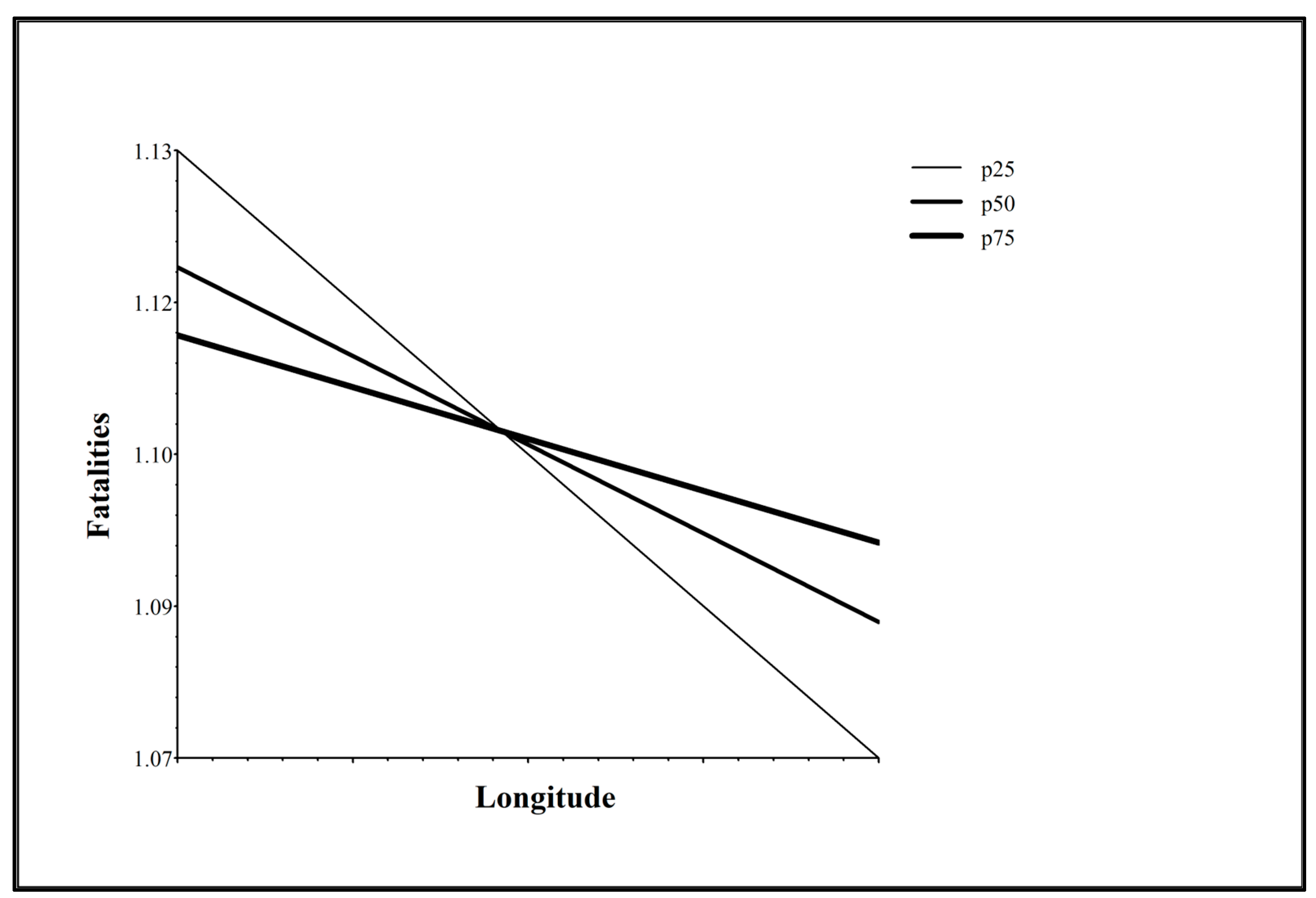
Figure 1 shows how the licensed drivers effect on fatalities changes by longitude in the contiguous United States. The negative slopes for the 25th (p25), 50th (p50), and 75th percentiles (p75) show that fatalities decrease from west to east. At the western longitudes of the contiguous United States, fatalities are highest in states where the licensed drivers per 1000 driving-age population are less numerous, such as in California. At the eastern longitudes of the contiguous United States, fatalities are highest in states where licensed drivers per 1000 driving-age population are more numerous, such as in Vermont. The point of intersection of the negative slopes for p25, p50, and p75 in Figure 1 represents the longitude where the licensed drivers effect is null in the contiguous United States. 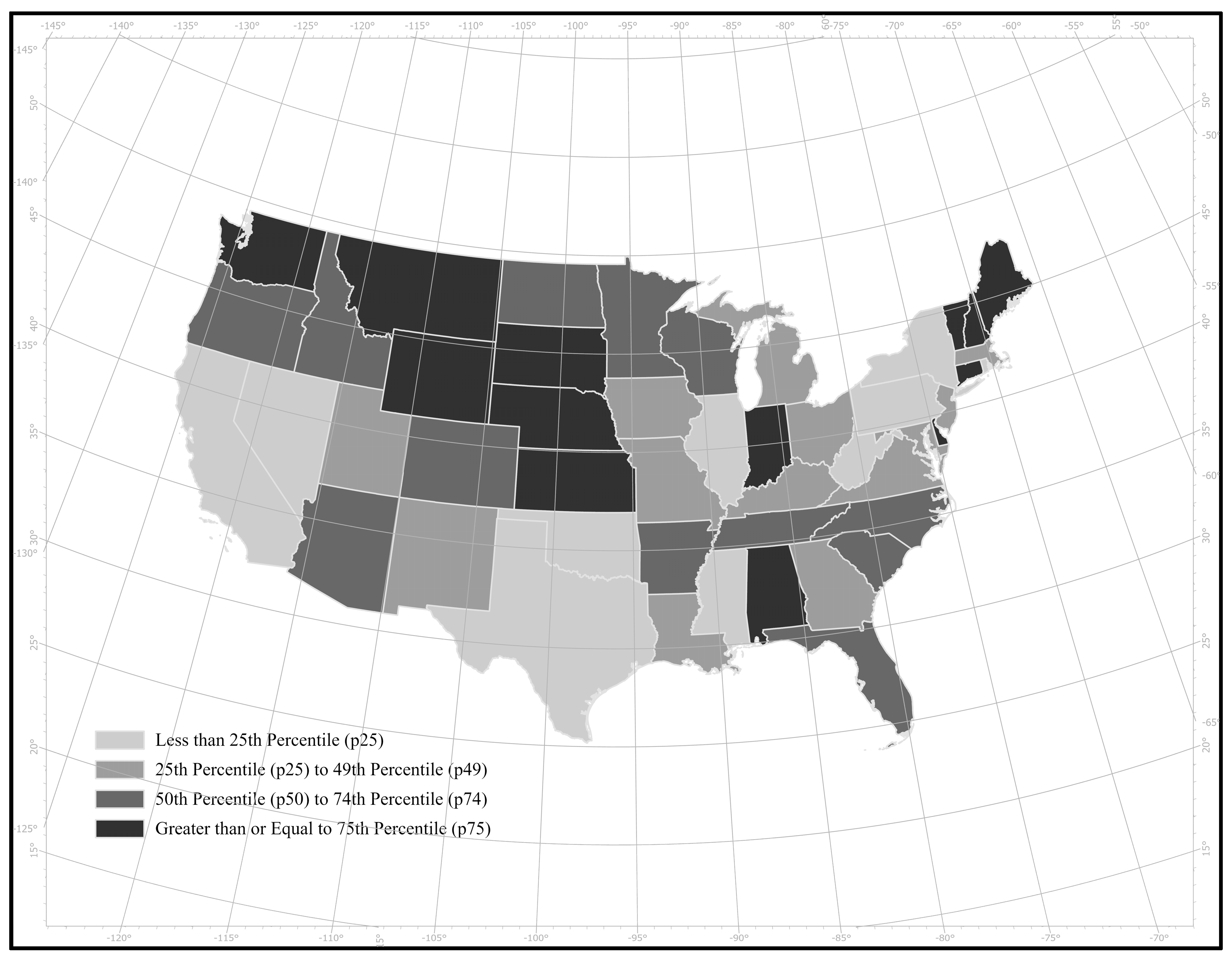Figure 2 is a choropleth map of licensed drivers per 1000 driving-age population in the contiguous United States. Manual classification represents the following four classes: less than 25th percentile (p25); 25th percentile (p25) to 49th percentile (p49); 50th percentile (p50) to 74th percentile (p74); and greater than or equal to 75th percentile (p75) of licensed drivers per 1000 driving-age population. Class breaks represent p25, p50, and p75 of the licensed drivers distribution. The graticule of longitudes in Figure 2 shows that the following states (from north to south) represent the geographic location from about −100 to −95 where the licensed drivers effect is null in the contiguous United States: North Dakota, Minnesota, South Dakota, Iowa, Nebraska, Missouri, Kansas, Oklahoma, and Texas.

5.4. Time Zones

The highest levels of aggregation are the most sensitive to sample size thresholds for accurate parameter and error estimates in full, multilevel models [22]. Since the respective sample sizes for states in the Pacific (4) and Mountain (7) time zones are insufficient, the results below are for the Pacific and Mountain, Central, and Eastern time zones, respectively.

Descriptive statistics for crashes and states in the Pacific and Mountain, Central, and Eastern time zones are in

Table 6. Descriptive statistics for time zones.

		Time Zone (n)
		Pacific and Mountain (125,160)		Central (223,283)		Eastern (289,721)
Level (n)	Variable	M 1	SD 2	M	SD	M	SD
Crash (638,164)
	Fatalities	1.10	0.40	1.11	0.41	1.09	0.35
	lnFatalities	0.06	0.22	0.07	0.23	0.05	0.20
	Alcohol	0.30	0.55	0.26	0.48	0.25	0.47
	DST (Percent)
	Yes	58.19		65.45		64.87
	No	41.81		34.55		35.13
	Drugs	0.09	0.32	0.08	0.30	0.09	0.30
	Latitude (Decimal Degrees)	+37.83	4.55	+35.58	4.84	+36.83	4.23
	Light (Percent)
	Yes	4.75		3.63		4.29
	No	95.25		96.37		95.71
	Longitude (Decimal Degrees)	−116.37	5.43	−92.83	4.57	−80.17	4.23
	Persons	2.68	2.02	2.51	1.86	2.49	1.79
	Vehicles	1.51	0.85	1.52	0.76	1.52	0.81
	Weather (Percent)
	Yes	13.64		19.32		20.88
	No	86.36		80.68		79.12
		Time Zone (n)
		Pacific and Mountain (11)		Central (16)		Eastern (22)
Level (n)	Variable	M	SD	M	SD	M	SD
State (49)
	Aggregate Travel Demand	94,050.90	146,701.55	94,710.32	89,777.87	103,391.03	81,824.57
	Licensed Drivers	906.93	35.46	908.37	48.97	899.16	60.83
	Motor Vehicle Crash Fatalities	699.35	978.00	807.76	786.65	767.67	687.54
	Aggregate Road Supply (Lane-Kilometers)	241,915.43	143,322.41	395,764.46	196,280.28	214,523.55	157,537.50
	Poor-Quality Road Surfaces (Percent)	5.53	5.17	7.05	3.80	13.07	17.12
	Registered Vehicles	2,570,613.89	4,709,974.36	2,125,533.57	2,013,478.82	2,714,141.22	2,171,491.90

¹ M = Mean. ² SD = Standard Deviation.

. The advantage of the decision to merge the states in the Pacific and Mountain time zones is accuracy in parameter and error estimation. The disadvantage of the decision to merge the states in the Pacific and Mountain time zones is heterogeneity in fatal motor vehicle crash outcomes. To test for intrazonal heterogeneity in the Pacific and Mountain time zones, descriptive statistics for the Pacific and Mountain, Pacific, and Mountain time zones are in

Table 7. Descriptive statistics for Pacific and Mountain, Pacific, and Mountain time zones.

		Time Zone (n)
		Pacific and Mountain (125,160)		Pacific (84,173)		Mountain (40,987)
Level (n)	Variable	M 1	SD 2	M	SD	M	SD
Crash (125,160)
	Fatalities	1.10	0.40	1.10	0.39	1.11	0.42
	lnFatalities	0.06	0.22	0.06	0.22	0.07	0.23
	Alcohol	0.30	0.55	0.28	0.51	0.33	0.64
	DST (Percent)
	Yes	58.19		63.96		46.36
	No	41.81		36.04		53.64
	Drugs	0.09	0.32	0.09	0.30	0.10	0.35
	Latitude (Decimal Degrees)	+37.83	4.55	+37.74	4.51	+38.01	4.62
	Light (Percent)
	Yes	4.75		4.53		5.21
	No	95.25		95.47		94.79
	Longitude (Decimal Degrees)	−116.37	5.43	−119.61	2.36	−109.72	3.59
	Persons	2.68	2.02	2.69	2.02	2.67	2.01
	Vehicles	1.51	0.85	1.52	0.88	1.50	0.79
	Weather (Percent)
	Yes	13.64		14.23		12.42
	No	86.36		85.77		87.58
		Time Zone (n)
		Pacific and Mountain (11)		Pacific (4)		Mountain (7)
Level (n)	Variable	M	SD	M	SD	M	SD
State (11)
	Aggregate Travel Demand	94,050.90	146,701.55	178,421.30	234,230.24	45,839.23	31,298.65
	Licensed Drivers	906.93	35.46	890.76	50.00	916.16	23.92
	Motor Vehicle Crash Fatalities	699.35	978.00	1216.14	1568.0	404.04	291.59
	Aggregate Road Supply (Lane-Kilometers)	241,915.43	143,322.41	316,646.40	219,082.81	199,212.02	66,228.58
	Poor-Quality Road Surfaces (Percent)	5.53	5.17	8.62	7.69	3.76	2.24
	Registered Vehicles	2,570,613.89	4,709,974.36	5,437,761.30	7,466,675.85	932,243.94	696,767.52

¹ M = Mean. ² SD = Standard Deviation.

. Intrazonal heterogeneity is only evident for DST in the Pacific (Yes = 63.96%, No = 36.04%) versus Mountain (Yes = 46.36%, No = 53.64%) time zones. So, the decision to merge the states in the Pacific and Mountain time zones probably fails to mask intrazonal heterogeneity in fatal motor vehicle crash outcomes. Indeed, multiple regression models of the crash-level independent variables reveal that the coefficient estimates for DST in the Pacific- and Mountain-time zone models are both positive, similar in magnitude (+0.30% versus +0.62%, respectively), and statistically significant. The following subsections present the random-intercept and -coefficients model results, respectively, for the Pacific and Mountain, Central, and Eastern time zones.

5.4.1. Random-Intercept Model Results for Time Zones

Estimates from random-intercept models for time zones are in

Table 8. Estimates from random-intercept models for time zones.

		Time Zone (n)
		Pacific and Mountain (125,160)		Central (223,283)		Eastern (289,721)
Level (n)	Variable	Fatalities 1	lnFatalities	Fatalities	lnFatalities	Fatalities	lnFatalities
Crash (638,164)
	Alcohol	+0.02 ***	+0.01 ***	+0.02 ***	+0.01 ***	+0.02 ***	+0.01 ***
	DST (Yes = 1, No = 0)	+0.01 **	+0.003 *	−0.02 ***	−0.02 ***	−0.02 ***	−0.02 ***
	Drugs	+0.03 ***	+0.02 ***	+0.03 ***	+0.02 ***	+0.03 ***	+0.02 ***
	Latitude (Decimal Degrees)	+0.01 ***	+0.003 ***	−0.000004	+0.0001	+0.002 ***	+0.001 ***
	Light (Dawn or Dusk = 1, Otherwise = 0)	+0.005	+0.003	+0.01 **	+0.01 **	+0.002	+0.001
	Longitude (Decimal Degrees)	+0.003 ***	+0.002 ***	−0.003 ***	−0.002 ***	−0.001 ***	−0.001 ***
	Persons	+0.08 ***	+0.04 ***	+0.08 ***	+0.04 ***	+0.06 ***	+0.03 ***
	Vehicles	−0.05 ***	−0.02 ***	−0.03 ***	−0.01 ***	−0.03 ***	−0.02 ***
	Weather (Adverse = 1, Otherwise = 0)	−0.002	−0.0003	+0.001	+0.001	+0.002	+0.001
		Time Zone (n)
		Pacific and Mountain (11)		Central (16)		Eastern (22)
Level (n)	Variable	Fatalities	lnFatalities	Fatalities	lnFatalities	Fatalities	lnFatalities
State (49)
	Intercept	+1.08 ***	+0.05 ***	+1.12 ***	+0.07 ***	+1.09 ***	+0.05 ***
	Licensed Drivers	−0.0004 *	−0.0002 *	+0.0001	+0.00005	+0.0001	+0.0001 *

¹ *** Significant at the 1.00% confidence level. ** Significant at the 5.00% confidence level. * Significant at the 10.00% confidence level.

. The left columns (Fatalities) present estimates for the number of fatalities. The right columns (lnFatalities) present estimates for the natural log of the number of fatalities. Consistent with expectations [13], fatalities increase as alcohol involvement increases in the Pacific and Mountain (by +1.00%), Central (by +1.00%), and Eastern (by +1.00%) time zones. Interestingly, fatalities increase slightly if the crash is in DST in the Pacific and Mountain (by +0.30%) time zones but decrease if the crash is in DST in the Central (by −2.00%) or Eastern (by −2.00%) time zones. Consistent with results for alcohol, fatalities increase as drug involvement increases in the Pacific and Mountain (by +2.00%), Central (by +2.00%), and Eastern (by +2.00%) time zones. Fatalities increase slightly as latitude increases from south to north in the Pacific and Mountain (by +0.30%) and Eastern (by +0.10%) time zones, but not the Central time zone. Interestingly, fatalities increase if the crash is at dawn or dusk in the Central (by +1.00%) time zone, but not the Pacific and Mountain or Eastern time zones. Fatalities increase slightly as longitude increases from west to east in the Pacific and Mountain (by +0.20%) time zone, but decrease slightly as longitude increases from west to east in the Central (by −0.20%) and Eastern (by −0.10%) time zones. Consistent with expectations, fatalities increase as the number of persons increases in the Pacific and Mountain (by +4.00%), Central (by +4.00%), and Eastern (by +3.00%) time zones. Surprisingly, fatalities decrease as the number of vehicles increases in the Pacific and Mountain (by −2.00%), Central (by −1.00%), and Eastern (by −2.00%) time zones. Fatalities decrease very slightly as licensed drivers increase in the Pacific and Mountain (by −0.02%) time zones but increase very slightly as licensed drivers increase in the Eastern (by +0.01%) time zone.

5.4.2. Random-Coefficients Model Results for Time Zones

Estimates from random-coefficients models for time zones are in

Table 9. Latitude and longitude estimates from random-coefficient models for time zones.

		Time Zone (n)
		Pacific and Mountain (125,160)		Central (223,283)		Eastern (289,721)
Level (n)	Variable	Fatalities 1	lnFatalities	Fatalities	lnFatalities	Fatalities	lnFatalities
Crash (638,164)
	Alcohol	+0.02 ***	+0.01 ***	+0.02 ***	+0.01 ***	+0.02 ***	+0.01 ***
	DST (Yes = 1, No = 0)	+0.01 **	+0.003 *	−0.005 ***	−0.003 ***	−0.002	−0.002 **
	Drugs	+0.03 ***	+0.02 ***	+0.03 ***	+0.02 ***	+0.03 ***	+0.02 ***
	Latitude (Decimal Degrees)
	Intercept	+0.002	+0.001	−0.0001	+0.00001	+0.002 ***	+0.001 ***
	Licensed Drivers
	Light (Dawn or Dusk = 1, Otherwise = 0)	+0.004	+0.003	+0.01 **	+0.01 **	+0.002	+0.001
	Longitude (Decimal Degrees)
	Intercept	+0.005 ***	+0.003 ***	−0.002 ***	−0.001 ***	−0.001 ***	−0.001 ***
	Licensed Drivers	−0.05 ***	−0.05 ***	+0.00001	+0.00001	+0.00002 ***	+0.00001 ***
	Persons	+0.08 ***	+0.04 ***	+0.08 ***	+0.04 ***	+0.06 ***	+0.03 ***
	Vehicles	−0.05 ***	−0.02 ***	−0.03 ***	−0.01 ***	−0.03 ***	−0.02 ***
	Weather (Adverse = 1, Otherwise = 0)	−0.002	−0.0002	+0.001	+0.001	+0.001	+0.001
		Time Zone (n)
		Pacific and Mountain (11)		Central (16)		Eastern (22)
Level (n)	Variable	Fatalities	lnFatalities	Fatalities	lnFatalities	Fatalities	lnFatalities
State (49)
	Intercept	+1.12 ***	+0.07 ***	+1.12 ***	+0.07 ***	+1.08 ***	+0.05 ***
	Licensed Drivers	+0.001	+0.0004	+0.0001	+0.00004	+0.0001	+0.0001 *

¹ *** Significant at the 1.00% confidence level. ** Significant at the 5.00% confidence level. * Significant at the 10.00% confidence level.

. The left columns (Fatalities) present estimates for the number of fatalities. The right columns (lnFatalities) present estimates for the natural log of the number of fatalities. The effects of licensed drivers on latitude and longitude are statistically significant in the Pacific and Mountain and Eastern time zones, but not the Central time zone. With regard to the former, the effect of licensed drivers on fatalities decreases very slightly as latitude increases from south to north in the Pacific and Mountain (by −0.01%) and Eastern (by −0.002%) time zones. The effect of licensed drivers on fatalities changes from Pacific and Mountain to Eastern time zones as longitude increases from west to east. The licensed drivers effect on fatalities decreases very slightly as longitude increases from west to east in the Pacific and Mountain (by −0.01%) time zones, but increases very slightly as longitude increases from west to east in the Eastern (by +0.001%) time zone.

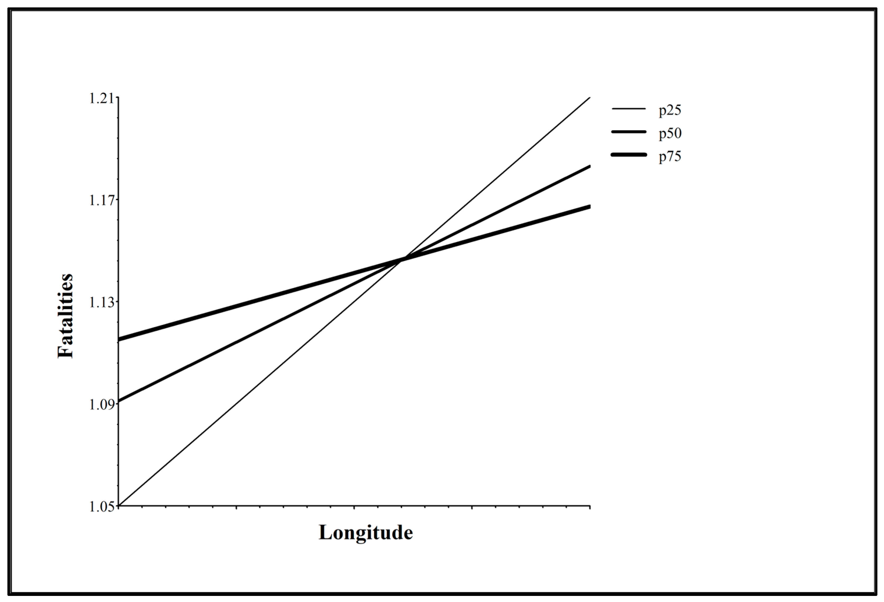
Figure 3 shows how the licensed drivers effect on fatalities changes by longitude in the Pacific and Mountain time zones. The positive slopes for p25, p50, and p75 show that fatalities increase from west to east in the Pacific and Mountain time zones. At western longitudes of the Pacific and Mountain time zones, fatalities are highest in states where licensed drivers per 1000 driving-age population are more numerous, such as in Washington. At eastern longitudes of the Pacific and Mountain time zones, fatalities are highest in states where licensed drivers per 1000 driving-age population are less numerous, such as in New Mexico. The point of intersection of the positive slopes for p25, p50, and p75 in Figure 3 represents the longitude where the effect of licensed drivers effect is null in the Pacific and Mountain time zones.

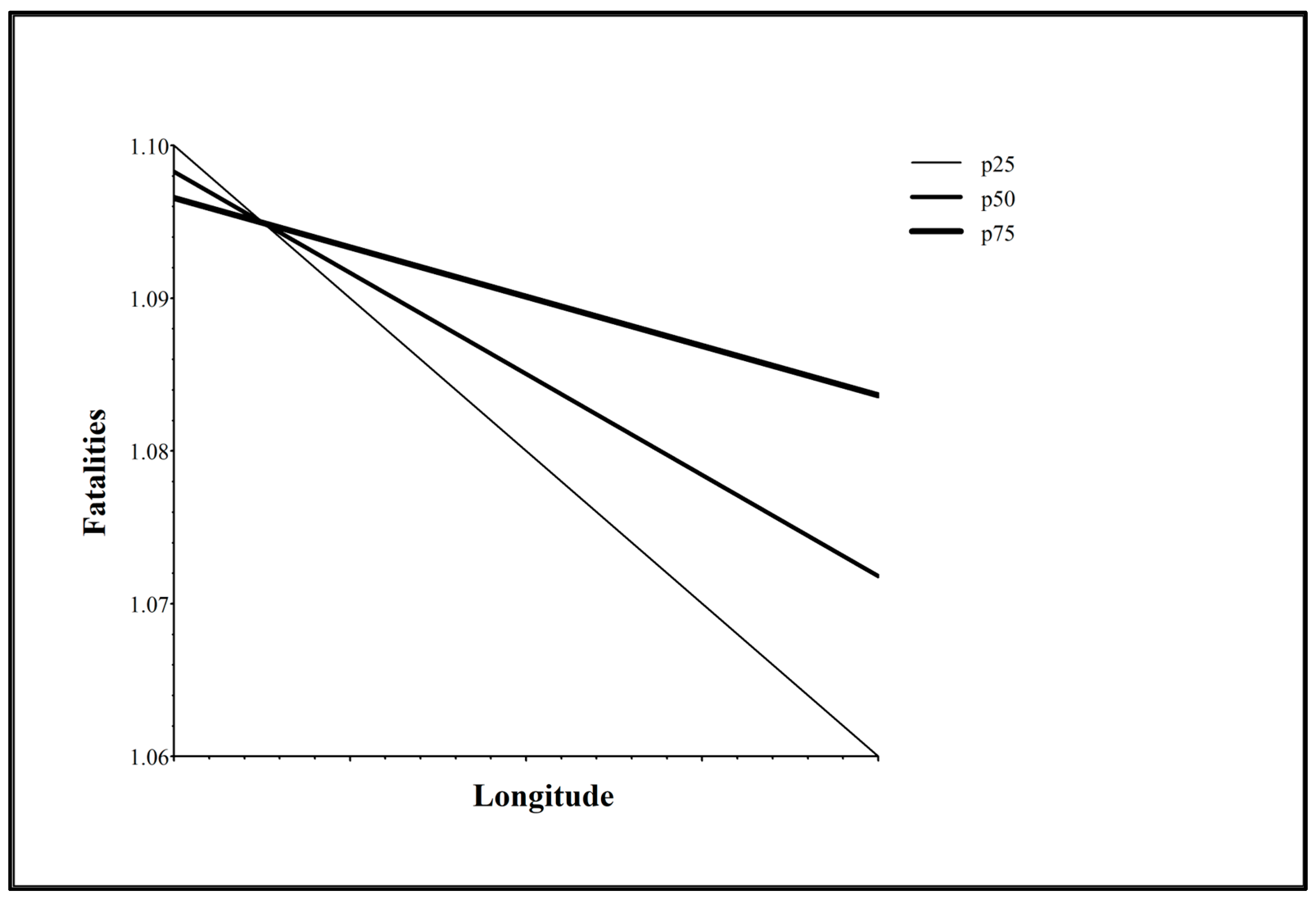
Figure 4 shows how the licensed drivers effect on fatalities changes by longitude in the Eastern time zone. The negative slopes for p25, p50, and p75 show that fatalities decrease from west to east in the Eastern time zone. At western longitudes of the Eastern time zone, fatalities are highest in states where licensed drivers per 1000 driving-age population are less numerous, such as in Kentucky. At eastern longitudes of the Eastern time zone, fatalities are highest in states where licensed drivers per 1000 driving-age population are more numerous, such as in Vermont. The point of intersection of the negative slopes for p25, p50, and p75 in Figure 4 represents the longitude where the licensed drivers effect is null in the Eastern time zone.

6. Discussion

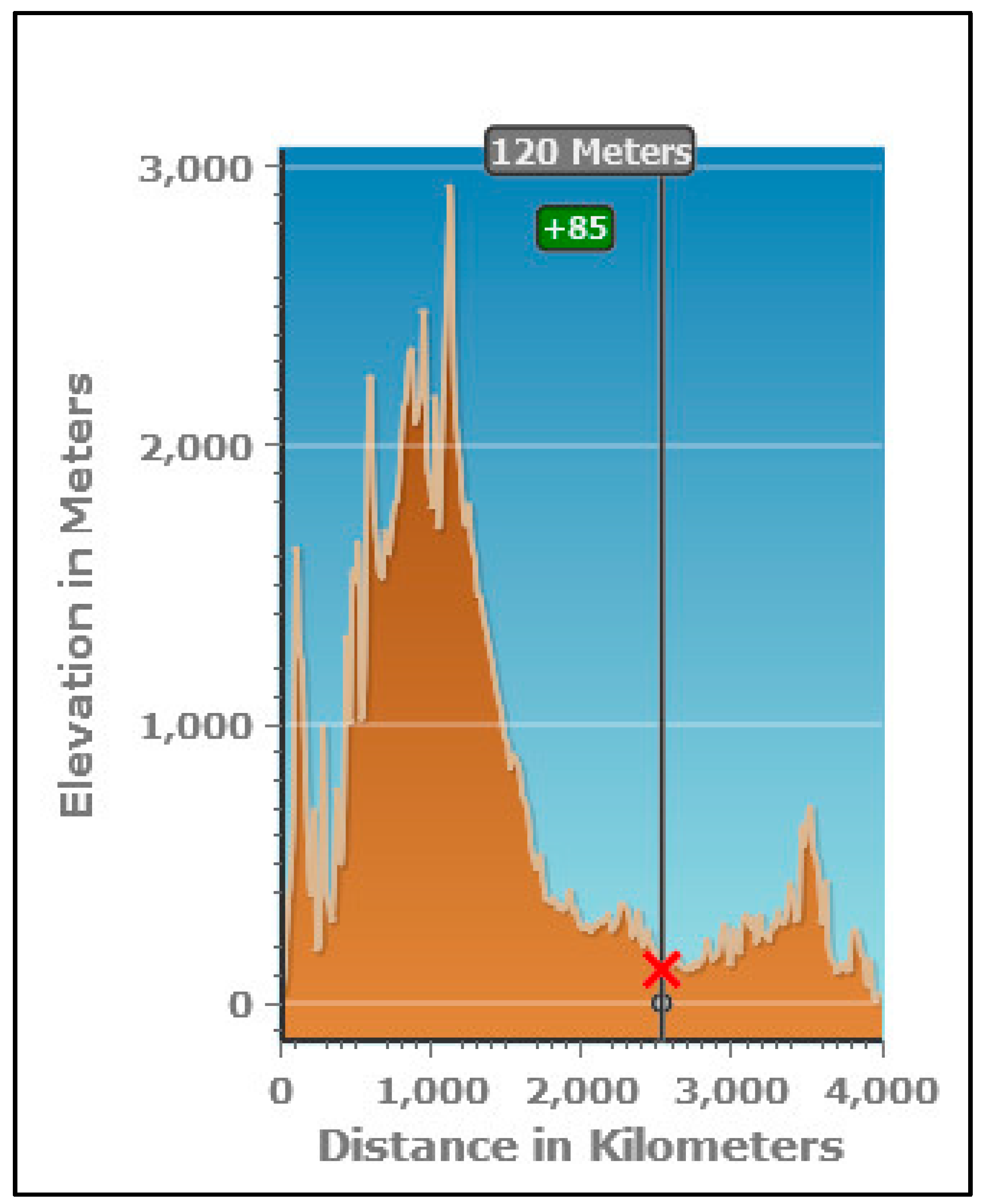
National (contiguous United States) and zonal (Pacific and Mountain, Central, and Eastern) analyses of DST-safety interactions reveal the following. The slight decrease in fatalities during DST in the contiguous United States masks an increase in fatalities during DST in the Pacific and Mountain time zones. The slight increase in fatalities during sunrise or sunset in the contiguous United States is representative of the increase in fatalities during sunrise and sunset in the Central time zone, not the Pacific and Mountain or Eastern time zones. The latter result is probably because of changes in relief from the Pacific and Mountain to the Central to the Eastern time zones (Figure 5). The slight increase in fatalities as latitude increases from south to north in the contiguous United States is representative of the slight increase in fatalities as latitude increases from south to north in the Pacific and Mountain and Eastern time zones, not the Central time zone. The latter result is probably because the clock times of sunrise and sunset vary more from season to season at northern latitudes in the contiguous United States at +49 than at southern latitudes in the contiguous United States at +25 [5]. For example, at +49 the clock time of sunrise ranges from about 0800 in January to about 0400 in June, but at +25 the clock time of sunrise ranges from about 0700 in January to about 0500 in June. In addition, at +49, the clock time of sunset ranges from about 0400 in January to about 0800 in June, but at +25, the clock time of sunset ranges from about 0500 in January to about 0700 in June. The time-zone effect in the contiguous United States, where fatalities increase from east to west (Figure 1), masks offsetting effects in the Pacific and Mountain time zones, where fatalities decrease from east to west (Figure 3), and the Eastern time zone, where fatalities increase from east to west (Figure 4). Interestingly, the magnitudes of the time-zone effects in this study are far lower than the magnitude of the time-zone effect in the literature of +4.00% per five-degree change in longitude from east to west in a time zone [6]. The magnitudes in this study are probably far lower because of dependent-variable and temporal-dimension differences. The dependent variable is the number of fatalities per crash event (fatal motor vehicle crash) in this study versus the incidence rate ratio in Fritz et al. [6]. The temporal dimension is the year in this study versus the week in Fritz et al. [6].

To return to the statistical problems with model specification, on the one hand, failure of full models of state-level independent variables to converge suggests that fatal motor vehicle crashes in terms of aggregate travel demand, motor vehicle crash fatalities, and registered vehicles are endogenous to DST-safety interactions. The latter result is inconsistent with the literature on the effect of traffic volumes on fatal crashes [3]. The result in this study is probably inconsistent because of measurement and methodology differences. This study uses aggregate travel demand to measure traffic volumes, while Fridstrøm et al. [3] use traffic counts to measure traffic volumes in Denmark and gasoline sales to approximate traffic volumes in Finland, Norway, and Sweden. Similar sources for the forty-eight states plus the one state equivalent (District of Columbia) in this study create one database amenable to exploration of both within- and between-state spatial and temporal variation. Dissimilar sources for the four countries in Fridstrøm et al. [3] create four databases amenable to exploration of only within-country spatial and temporal variation. Therefore, the effect of traffic volumes on fatal crashes is fixed from country to country in Fridstrøm et al. [3], which is theoretically and empirically implausible.

On the other hand, the fact that models with information on differences from state to state in fatal motor vehicle crashes in terms of licensed drivers successfully converge is worthy of discussion. Clearly, fatal motor vehicle crashes in terms of licensed drivers effectively, if not modestly, explain spatial heterogeneity in the crash-level data. State governments, not the federal government, regulate operator licensure. Policy implications for state governments to intervene on fatal motor vehicle crashes in terms of licensed drivers are as follows [17]. First, temporary or permanent licensure forfeiture for drivers whose records of alcohol and/or drug impairment are known to law enforcement. Second, interdiction by law enforcement where impairment from alcohol and/or drugs among drivers is prevalent. The spatiotemporal specificity of the zonal analyses suggests that law enforcement target licensed drivers at northern latitudes of the Pacific and Mountain time zones during DST; licensed drivers in the Central time zone at dawn or dusk before or after DST; and licensed drivers at northern latitudes in the Eastern time zone before or after DST to decrease the lethality of motor vehicle crashes. Policy implications of the national DST-safety benefit are consistent with Ferguson et al. [8]. That is, the probability of one more fatality decreases slightly in the contiguous United States (by −0.10%) in DST. However, national DST-safety benefits mask interzonal differences. That is, the probability of one more fatality decreases in the Eastern and Central time zones (by −2.00%) but increases slightly in the Pacific and Mountain time zones (by +0.30%) in DST. All else equal, national DST-safety benefits mask zonal DST-safety costs in the Pacific and Mountain time zones.

7. Conclusions

The contributions of this study derive from measurement and methodological advancements to the literature on DST-safety interactions. Twenty years of data on fatal motor vehicle crash severity contextualize DST-safety interactions in the contiguous United States from 2001 to 2020. Adoption of a multilevel approach unmasks within- and between-time zone differences in DST-safety interactions. Subsequent analyses answer a call [6] in the literature to control for geographical differences [4] in DST-safety effects. Results from national and zonal analyses of fatal motor vehicle crash severity help to contextualize DST-safety interactions, which are, at best, inconsistent in the literature. The limitation of this study is as follows. Police reports of alcohol involvement in FARS [18] are frequently missing. So, the present study undercounts the number of persons whose police reports indicates alcohol involvement. To that end, coefficient estimates for alcohol in the national and zonal analyses are probably low in magnitude.

The trajectory of ongoing research is as follows. Research on DST-safety interactions in the counties/county equivalents the present study excludes is ongoing. Exclusion of counties/county equivalents due to time-zone divisions and changes limits the generalizability of the results. Such research is important to generalize the results to the contiguous United States. Research to estimate missing Blood Alcohol Concentration (BAC) values for persons in FARS via multiple imputations [24,25] is also ongoing. Estimation of missing BAC values is important to accurately and precisely estimate the magnitude of the alcohol involvement-effect on fatal motor vehicle crash outcomes regardless of DST-safety interactions. Finally, further research on the DST-transition effect is ongoing. Specifically, a multilevel approach to fatal motor vehicle crash outcomes before and after DST transitions where the temporal dimension is hours, days, weeks, or months is important to further contextualize such outcomes.