Flight Scheduling for Transportation of Packages Between Logistics Bases Using Drones

Abstract

In recent years, interest in drone-based logistics has grown due to the increasing demand for efficient and sustainable package transportation, driven by the expansion of e-commerce and rising environmental awareness. In this study, we focus on flight scheduling for the efficient transportation of packages between logistics bases, rather than on last-mile delivery. In scenarios where the number of packages handled at each base varies, efficient transportation can be achieved by having drones visit high-demand bases more frequently. To this end, we consider a system with two types of drones: local drones that visit all bases, and express drones that visit only selected high-demand bases. We formulate this problem as a mixed integer linear programming (MILP) model that minimizes the total transportation time. This model simultaneously determines which bases should be visited frequently and computes flight schedules that enable efficient package delivery. Unlike existing transportation models that assume fixed linear routes, our model allows for flexible routing, including direct flights and loop-based paths between bases. To ensure scalability, we also propose an approximation method that significantly reduces the computational cost. As the number of logistics bases increases, the exact solution of the MILP becomes intractable. Therefore, we pre-select candidate high-demand bases based on package volume and spatial layout, thereby reducing the number of decision variables. This makes it possible to compute high-quality solutions even in large-scale environments. Through numerical experiments, we show the effectiveness of our proposed methods for the transportation of packages between logistics bases.

1. Introduction

In recent years, there has been a growing interest in the use of drones for logistics [1,2,3,4,5,6,7,8]. This is caused by the need for the more efficient transportation of packages because logistics is becoming more active around the world with the spread of electronic commerce sites and people’s growing awareness of environmental issues. Drones can transport packages in a shorter time than trucks because they are not affected by traffic congestion or road conditions [1,4]. Additionally, drones do not emit harmful substances into the environment because they are generally battery-powered [2,3,4].

Many studies have been conducted on the use of drones in logistics, most of which have considered the last-mile delivery problem [1,2,3,4,5,6,7,8], which relates to the final stage of the manner in which a package is delivered to its destination (Figure 1). By contrast, few studies have been conducted on the use of drones not in the last mile, but between points where packages are picked up and delivered, that is, between logistics bases. As mentioned above, it is important to study the use of drones between logistics bases given the current scenario of active logistics and environmental issues.

In this study, we consider a scenario in which drones transport packages between logistics bases (Figure 1). Specifically, in an area with many logistics bases, multiple drones visit each base to transport packages that have been left at each base by senders to the nearest base of each destination (Figure 2). As shown in Figure 2, if the number of packages handled by each base is different, the method by which each drone visits all bases is considered to be inefficient. Therefore, it is necessary to consider how the drones should be flown to transport packages efficiently.

To transport packages efficiently, we consider a system in which drones frequently visit bases with a large number of packages. Specifically, a good approach may be that two types of drones are flown: drones that visit all bases within an area and drones that visit only bases with a large number of packages. These bases should be chosen carefully because the transportation time between each base varies greatly depending on the choice of bases to be visited frequently. Such a problem is similar to the problem of determining the stops of “express trains” that only stop at stations on a railroad with a large number of passengers. The time required for passengers to travel between each station on the line varies greatly depending on where express trains stop. In recent years, in some studies, authors have focused on the problem of determining the stops of express trains using a mathematical optimization problem [9,10,11]. In [10], an optimization problem was proposed to minimize the total travel time of all passengers on a straight line, assuming that both express and local trains are running on that line. By solving this problem, the authors demonstrated that it is possible to calculate a timetable (diagram) that optimizes the stops of express trains. We can incorporate with this previous study to solve the drone delivery problem.

Therefore, as a proposed method, we formulate a mixed integer linear programming problem (MILP) to calculate the flight schedules of drones, referring to the previous study on efficient passenger transportation on a railroad. Specifically, we replace the terms “line”, “stations”, “trains”, and “passengers” in [10] with “flight route”, “logistics bases”, “drones”, and “packages”, respectively, and formulate an MILP that minimizes the transportation time of packages between each base. By solving this problem, we optimize which bases to visit frequently and calculate flight schedules for efficient package transportation using drones. The difference between [10] and this study is that we do not predetermine the flight route, whereas the railroad was determined. As shown in Figure 3a, express trains and local trains run on the same line; hence, express trains run via stations where they do not stop. By contrast, because drones fly in the air, they can select more flexible routes than trains that run only on a predetermined line. Another difference is that, in [10], a straight line is assumed, whereas in this study, the flight route is circular, as shown in Figure 2. Based on these differences, it is necessary to study the formulation of flight routes and flight schedules to enable the more efficient transportation of packages.

To solve the unique problems of the drone route problem, in the proposed method, we formulate flight schedules for drones that visit only some bases, assuming that they fly only through the bases that they visit. As shown in Figure 3b, drones fly in a straight line between the bases they visit and do not pass through the other bases. In the train problem [10], express and local trains run on the same line; hence, there are arrival and departure times at all stations, including the stations that express trains pass through. Therefore, an arrival time of express trains at each station is the time of departure from the previous station plus the time required between stations. A departure time is the arrival time plus the stopping time at the station. However, when determining the departure time of a transit station, the stopping time is not added. By contrast, in the drone problem, drones visit only a subset of bases; hence, arrival and departure times are not necessary for the bases that drones do not visit. Furthermore, the arrival and departure times of drones cannot be obtained by the aforementioned addition methods because which bases the drones visit is unknown at the time of the formulation of the MILP. Therefore, in the proposed method, we consider variables and constraints for formulating arrival and departure times. We also consider various other variables and constraints to address the differences from [10], such as the fact that the flight routes of drones are circular.

Although we can obtain a strict solution by formulating the MILP, the computational cost is much higher than that for the train problem because we add various constraints. To overcome this difficulty, we propose an approximate solution method by determining which bases to visit frequently based on the layout of the logistics bases and the number of packages at each base. Specifically, we focus on the fact that the computational cost required to solve an optimization problem generally depends on the number of decision variables. In the proposed MILP, the decision variables are which bases are to be visited frequently. Therefore, determining these bases in advance reduces the number of decision variables, thereby reducing the computational cost.

In this study, we demonstrate through numerical experiments that the proposed method can be used to transport packages efficiently. Furthermore, we demonstrate that the proposed approximate solution method can achieve the same level of transportation efficiency as the exact solution of the MILP and significantly reduce the computational cost of the exact solution method.

The contributions of this study are summarized as follows:

• We consider a system in which drones transport packages between logistics bases. In most studies on package delivery by drones, the authors focused on the “last mile” problem and very few considered transportation between bases. In this study, we consider the number of packages handled at each base, and drones transport them while frequently visiting some bases with the largest number of packages. This system is useful when considering how drones should be flown to transport packages efficiently between logistics bases in the future, when drones capable of transporting a large number of packages over long distances are developed. Solving such inter-base scheduling problems effectively is expected to be highly valuable for logistics providers, as it can support the practical implementation of scalable and efficient drone delivery operations beyond the last mile.
• To transport packages efficiently, we propose an MILP that minimizes the transportation time of packages between each base. Solving this problem optimizes which bases to visit frequently, and we calculate flight schedules for the efficient transportation of packages by drones. By solving this MILP, we can calculate flight schedules that optimize the bases frequently visited by drones. Additionally, we can calculate flight schedules for loop routes, and scenarios in which drones fly in a straight line between each base they visit and where they do not fly via other bases. These points differ significantly from the railroad study referenced in the formulation of the MILP. That study assumed that all trains run on a single straight line.
• We propose an approximate solution method for the MILP. This MILP has the disadvantage that as the number of assumed logistics bases increases, the computational cost to compute the exact solution becomes generally huge. Therefore, we determine which bases drones visit frequently based on the layout of bases and the number of packages at each base. This reduces the number of decision variables in the MILP, thus reducing the computational cost required to solve it. Thus, even in a scenario with a large number of bases, the MILP can be solved with a realistic computational cost.

The remainder of this paper is structured as follows: In Section 2, we introduce previous studies on the use of drones in logistics and on the calculation of railway diagrams based on mathematical optimization problems. In Section 3, we present a system model for the transportation of packages and flight schedules of drones, and explain the scenario setting assumed in the proposed method. In Section 4, we present the objective function and constraint conditions of the proposed MILP. In Section 5, we describe a solution method to compute an approximate solution of the proposed MILP in a short time. In Section 6, we describe the numerical experiments we conducted to evaluate the performance of the proposed MILP and its approximate solution method. Finally, in Section 7, we present the conclusions of this study.

2. Related Work

In this section, we introduce previous studies on the use of drones in logistics in addition to previous studies on the calculation of a railway diagram using an optimization problem. Previous studies on drones are classified into two categories: those that assume the delivery of packages in the last mile and those that do not. In previous studies on railways that focused on minimizing the travel time of passengers, various approaches were introduced for calculating diagrams, such as minimizing the number of trains required for a commercial operation.

2.1. Previous Studies on the Use of Drones in Logistics

In recent years, researchers have been active in studying the use of drones in logistics. Most researchers have been concerned with improving the efficiency of last-mile delivery. This is because the upper limit of the package carrying capacity and the maximum distance over which a typical drone can fly continuously are much smaller than those for trucks and freight trains. In this section, we introduce the studies in [12,13,14,15,16,17,18]. Among these, refs. [12,13,14,15,16,17] are related to the last-mile problem, and in [18], base transportation was considered. This literature can be broadly categorized into three areas: truck- and train-assisted drone delivery systems, stand-alone last-mile drone delivery systems, and inter-base drone logistics.

2.1.1. Truck- and Train-Assisted Drone Delivery Systems

Several studies have explored hybrid systems that combine traditional transport modes with drones to improve last-mile delivery efficiency. In [12], a combination of a truck and a drone were considered for deliveries. Similar studies have been conducted actively in recent years [7,19,20,21,22]. A truck departs from a logistics base with packages and a drone. While the truck is delivering a package to one destination, the drone takes off from the truck and delivers a package to another destination in the vicinity, thereby making the delivery more efficient than using a truck alone. Two problems were proposed: minimizing the cost of batteries and other equipment needed to fly the drone, and minimizing the time required for the drone to make deliveries. By solving these problems, researchers demonstrated that it was possible to calculate both the number of drones required to accompany one truck and the optimal flight route of the drone.

In [13], the authors investigated a delivery system that combines rail transport and drone operations, which resembles models for combined truck and drone delivery. In this system, a train carries a drone along with packages. When the train approaches a delivery destination, the drone takes off to deliver a package. When the delivery is complete, the drone returns to the train and continues toward the next delivery point. Because the train makes scheduled stops at stations, the drone can always catch up with it. In [13], the authors proposed a problem to minimize the total time from the train’s departure from the starting station until the drone completes all deliveries. By solving this problem, the authors demonstrated how to compute optimal solutions for the timing of the drone’s takeoff and landing, in addition to its flight routes.

2.1.2. Stand-Alone Last-Mile Drone Delivery Systems

Many studies have investigated the design and optimization of autonomous drone operations in last-mile scenarios without relying on trucks or trains. In [14], the authors examined how the flight speed of a drone is influenced by the weight of the packages being delivered and emphasized the need to construct delivery routes that account for this factor. A single drone departs from a logistics base carrying packages for multiple destinations, within its maximum payload capacity. The drone visits each destination once, delivers a package, and then returns to the logistics base. Because the flight speed of drones typically decreases as the payload weight increases, the authors proposed a problem focused on minimizing the total delivery time rather than the total flight distance. The findings demonstrated that prioritizing destinations with heavier packages led to a more efficient route compared with simply following the shortest route.

In [15], the authors conducted a numerical experiment assuming that deliveries are made in Milan, Italy, by assigning specific values to the size of the drone, its flight speed, the upper limit of the payload capacity, the distance it can fly, and the time required to charge the battery, based on the performance of a modern general drone. Based on the set drone flight performance, multiple logistics bases are set up so that drones can deliver throughout the city of Milan, and one drone is deployed at each base. It is not possible to attach packages to a drone for multiple simultaneous deliveries to various destinations. Therefore, the delivery model is simply that each drone repeatedly travels back and forth between a single delivery location and a logistics base. Because the drone’s flight performance is set in detail and the experiment assumes delivery in a real city, this study is of great help in the practical application of last-mile packages delivered by drones.

In [16], the authors investigated a delivery system involving multiple drones operating from a single logistics base to numerous delivery destinations. Each drone can carry multiple packages within its maximum payload capacity. Because the number of destinations exceeds the number of available drones, the destinations are divided into several groups, with one drone assigned to each group. In each group, the drone follows the shortest possible route to visit all assigned destinations. The focus of the study is to determine the optimal number of groups, which corresponds to the number of drones required. This optimization considers constraints such as ensuring that the total number of packages delivered to each group does not exceed the payload capacity of the drones and that the travel distance for visiting all destinations remains within the drones’ maximum flight range. The objective is to minimize overall costs, including battery and maintenance expenses, while also reducing customer waiting times for package delivery.

In [17], the authors considered the last-mile delivery problem. This study is somewhat similar to our study in that it assumes that drones deliver packages from logistics bases to customers and simultaneously collect packages from customers and transport them to logistics bases. In an environment with multiple logistics bases, customers, drones, and packages, each drone belongs to one of the bases, and each package is waiting at one of the logistics bases or at the customer. The destination customer for each package waiting at logistics bases and the destination logistics base for each package waiting at customers are determined. The packages are transported by one drone, which cannot carry more than one package at a time. Therefore, drones cannot collect packages in succession, but they can visit multiple points, such as making a delivery to one customer and then going to another customer to collect a package, provided the flight distance does not exceed the drones’ flight limit. Additionally, drones can deliver packages to logistics bases that are different from their own. The main objectives of the study are to determine which drone transports which package and the optimal flight route for each drone. The authors proposed a problem to collaboratively minimize the total flight distance of each drone and the total number of packages transported by each drone.

2.1.3. Inter-Base Drone Logistics

Few studies have examined the use of drones for transportation between logistics bases, rather than last-mile delivery. [18] is one of the few studies that assumes the use of a drone in transporting packages between logistics bases rather than the last mile. In that study, the use of a drone capable of carrying a large number of packages simultaneously over a long distance is assumed. Specifically, it is a large drone called an unmanned cargo aircraft with a maximum payload capacity of 1 ton. This drone is currently under development and when put into practical use will be able to operate as a drone for transporting packages between logistics bases. Furthermore, the drone can be equipped with a function that automatically loads and unloads packages, which makes it possible to transport packages to locations that are not equipped with ground facilities. In this study, we assume the use of such drones and consider how to operate drones to achieve the efficient transportation of packages between logistics bases.

Thus, while extensive research has been conducted on last-mile drone delivery, studies focusing on drone-based inter-base logistics transportation remain limited. However, as the use of drones in logistics is expected to expand significantly beyond the last mile in the coming years, it is essential to explore their potential in inter-base operations. Investigating such mid-mile applications is therefore of great importance for the development of comprehensive and scalable drone logistics networks.

Furthermore, compared to ground vehicles constrained by road networks, drones can freely determine their flight paths, which introduces additional flexibility but also increases the complexity of scheduling. This highlights the importance of effective scheduling methods to fully leverage the potential of drone-based inter-base logistics.

2.2. Previous Studies on Railway Diagram Calculation

In [9,10,11], the problem of minimizing the total travel time of passengers on a line was proposed, which is closest to the method proposed in this study. The line has local trains that stop at all stations and express trains that stop only at some stations, and the focus is on the optimization of the stops of express trains. Because the time required between each station varies depending on the stops of express trains, the fastest travel times for passengers traveling between stations are formulated, taking into account the possibility of express trains stopping or passing at all stations and the connections with local trains at the stops of express trains. The proposed method in each reference is an optimization problem that minimizes the sum of all these times. By solving this problem, the authors demonstrated that the optimal solution can be calculated for the stops of express trains, the dwell time of trains at each station, and the headway between local and express trains, and that a demand-compatible diagram can be calculated.

In [23,24], the problem of maximizing the profit earned by a railway company through commercial operations was proposed. Many trains run on a line throughout one day. The setting is that the stops along the line vary from train to train, and the stops are optimized for each train according to demand. Sales revenues, such as fare revenue, are formulated by considering whether each train stop satisfies the demand at each station. The authors demonstrated that a demand-compatible diagram can be calculated by maximizing the profit obtained by subtracting the cost of operating the trains, such as electricity, from the sales revenues.

In [25,26,27,28], the problem of collaboratively minimizing two factors was proposed: the headway between two consecutive trains and the number of trains required for a day’s operation. These two factors are in a trade-off relationship, which poses a major issue for railway companies as they plan their operations and purchase trains. Specifically, the smaller the headway, the more convenient it is for passengers, but this requires a larger number of trains. Conversely, if the number of trains is small, the headway increases and passenger convenience decreases. To resolve this issue, in [25,26,27,28] a method was proposed to increase the utilization ratio of each train to the limit and to operate a large number of services with a small number of trains.

In [29], an optimization problem was proposed to adjust an already calculated diagram to match demand using constant values such as the arrival and departure times of each train at each station. Specifically, the deviation between the original and adjusted diagrams for the departure and arrival times of each train at each station; the number of passengers left unloaded when each train departs from each station; and the energy required to run the trains, such as electricity, are minimized in a collaborative manner. In particular, the unloading of passengers occurs when the number of passengers waiting for a train at a station exceeds the number of passengers that the train can accommodate, that is, the capacity of the train minus the number of passengers on board. Therefore, during times when unloading is likely to occur, adjustments are made to reduce the headway between trains.

3. System Model and Flight Schedule

Suppose that there are many logistics bases, as shown in Figure 4, and drones transport packages picked up at each base to another base. The number of bases is N, and each base is assigned a number from 0 to $N-1$. Base 0 is the terminal point of the drone’s one revolution around the flight routes. Figure 4 shows the scenario when $N=8$ as an example. Let $\mathcal{N}=\{0,1,\dots ,N-2,N-1\}$ be the set of logistics bases. In this paper, the numbering of the bases from 1 to $N-1$ (excluding base 0) is determined based on the solution of the traveling salesman problem, formulated as an integer linear programming problem. The traveling salesman problem identifies the shortest route that visits all bases exactly once, and we assign the numbers in the order the bases appear along this optimized route starting after base 0.

There are multiple destinations and senders of packages in the vicinity of each base, and packages are constantly being delivered to and from their nearest bases. The packages transported by drones to each base are delivered to their destinations and new packages are delivered to each base from senders. The number of these packages is “the number of packages handled at each base”. The number of packages handled at each base is assumed to vary. Let $W_{i,j}$ be a constant that represents the total number of packages transported from base i ($i\in \mathcal{N}$) to another base j ($j\in \mathcal{N}\backslash \left\{i\right\}$) in the time from the start of the first drone flight to the end of the last drone flight.

In this study, we assume a scenario in which two types of drones fly. The first type visits all bases in ascending order of base number as determined by the solution of a traveling salesman problem. The second type of drone visits only bases that handle a large number of packages in ascending order of base number and does not fly to other bases. Because these are similar to a local train and express train on a railroad, we call the first type a “local drone” and the second type an “express drone”. Express drones fly in a straight line between the bases they visit. Because the flight routes of local drones and express drones are different, we denote the route of local drones by ${\mathcal{P}}_L$ and the route of express drones by ${\mathcal{P}}_X$ to distinguish between them. Figure 4 shows, as an example, that express drones visit bases 0, 2, 5, and 6. Because base 0 is a terminal point, express drones always visit base 0. Therefore, base 0 is assumed to handle the largest number of packages among the bases in $\mathcal{N}$.

In this study, multiple flights of local drones and express drones occur on their respective routes at constant intervals. The bases visited by express drones are also assumed to be constant. Local drones and express drones depart from base 0 every $H_W$ time units, and the first local drone departs from base 0 at time 0, where $H_W$ is a constant that represents the flight interval. Furthermore, express drones always depart from base 0 at time $\eta$ later than local drones. $\eta$ is one of the decision variables of the proposed MILP and is a value between 0 and $H_W$. The time at which the k-th local drone or the k-th express drone departs from base 0 is expressed as the following equations, respectively:

$$\begin{array}{cc}\hfill \mathrm{Local}\mathrm{drones}:& (k-1)H_W(k\in \mathbb{N}),\hfill \end{array}$$

(1)

$$\begin{array}{cc}\hfill \mathrm{Express}\mathrm{drones}:& (k-1)H_W+\eta (k\in \mathbb{N}),\hfill \end{array}$$

(2)

where $\mathbb{N}$ is the set of natural numbers. After local drones and express drones return to base 0 after completing one round of their respective flight routes, they start their next itinerant flights without changing their own types or routes. In this case, the dwell time by drones at base 0 is adjusted so that the departure time for each type of drone is as shown in Equations (1) and (2).

Figure 5 shows an example of the flight schedules of drones calculated using the proposed method. A flight schedule is a graphical representation of drones on a plane with the horizontal axis representing the time and the vertical axis representing the number of logistics bases. The solid red lines in the figure represent the flight schedules of express drones, and the dashed black lines represent the flight schedules of local drones. In Figure 5, as an example, express drones visit bases 2 and 5, in that order.

Local drones and express drones exchange packages with each other at each logistics base. Specifically, at the bases visited by express drones, some packages are passed to a local drone at the same time as an express drone loads or unloads. Additionally, some packages are passed from a local drone to an express drone. This exchange of packages enables efficient transportation. As an example, we consider the case in which packages are transported from base 1 to base 5 in the flight schedules shown in Figure 5. Because no express drone visits base 1, the packages are loaded onto a local drone at base 1, but express drones visit base 2 on the way, and the packages can be switched from the local drone to the express drone at base 2. Note that base 5 at the destination is also visited by express drones. Furthermore, as shown in Figure 5, we note that express drones overtake local drones in the section from base 2 to base 5 on the timetable. Therefore, using an express drone to transport packages along the section from base 2 to 5 reduces the travel time compared with using a local drone to transport packages along the entire section from base 1 to 5. Similarly, when packages are transported from base 0 to base 4, the time required is reduced by reloading some packages at base 2. In this case, at base 2, the packages are transferred from an express drone to a local drone. Thus, cooperation between express drones and local drones to exchange packages is similar to the case on a railroad where an express train connects with a local train at a station, where both trains stop and passengers change between the two trains. Hereafter, we refer to the coordination between express drones and local drones as a “connection”.

For simplicity, we assume that the drones are equipped with sufficiently large batteries and that crashes caused by energy depletion do not occur. Furthermore, we assume that the maximum number of packages that can be carried by drones is sufficiently large and that all packages that must be carried at each base can be loaded. However, it is important to consider these factors when considering realistic drone transportation problems, and further study on this is needed in the future.

4. Proposed Method: MILP to Calculate Flight Schedules

In this section, we introduce the outline of the proposed method in Section 4.1, define the objective function in Section 4.2, and present the constraints in Section 4.3.

4.1. Outline

We formulate an MILP as the proposed method to calculate flight schedules by optimizing which bases express drones visit and the headway (departure interval) $\eta$ between each local drone and each express drone at base 0. We define a binary variable $x_j$ that is 1 if express drones visit base j and 0 if they do not. Furthermore, because flight scheduling is tantamount to calculating the departure and arrival times of the drones at each base, we denote the departure times of the first flight of the express and local drones at base j by $a_j^X,a_j^L$, respectively, and denote the arrival times by $d_j^X,d_j^L$, respectively. Because the first local drone departs from base 0 at time 0 and the first express drone departs from base 0 at time $\eta$, they are represented as $d_0^L=0,d_0^X=\eta$, respectively.

To formulate an MILP for which an optimal solution exists, we calculate flight schedules considering the smallest increment in the timetable. As described in Section 3, the variable $\eta$ has the constraint $0\le \eta <H_W$, which includes an inequality without an equals sign; that is, the feasible region is an open set, which may result in an MILP with no optimal solution. Therefore, we define a constant $I_C$ that represents the smallest increment in the timetable, and the flight interval $H_W$ and the departure and arrival times $a_j^X,a_j^L,d_j^X,d_j^L$ are all multiples of $I_C$. This makes the constraint $0\le \eta \le H_W-I_C$, and the feasible region is a closed set. Note that we should set $I_C$ to an integer value in principle, such as 10 s or 1 min.

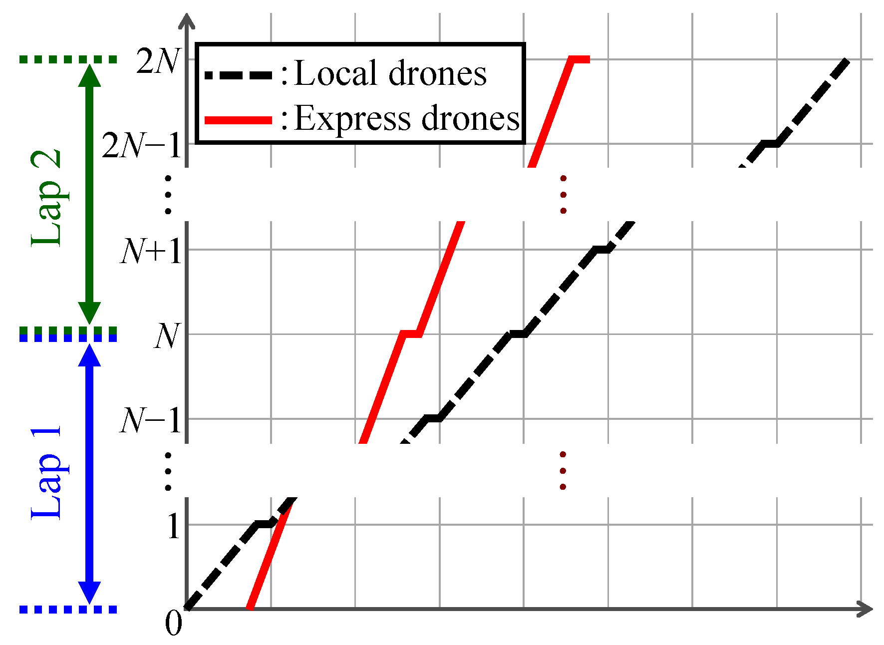
To consider the transportation of packages between all bases, we calculate the flight schedules of two laps for local drones and express drones (Figure 6). The two-lap calculation allows for the consideration of transportation that spans from base 0 to the next itinerant flight across base 0, for example, from base $N-1$ to base 1. For convenience, we denote the numbers of the bases to be visited in the second round by $N,N+1,\dots ,2N$. Figure 6 shows examples of flight schedules for two laps of routes and the graphs of a local drone and express drone on the first flight.

By considering the flight schedules for two laps of routes, we can formulate the proposed method as an MILP using [10] on railways. The constants and sets are listed in

Table 1. Constants and sets used in the MILP formulation. (a) Constants; (b) Sets.

(a)
Symbol	Meaning
N	Number of logistics bases.
$W_{i,j}$	Number of packages whose source base is i and destination base is j.
$I_C$	Smallest increment in a flight schedule. Fixed integer value.
$T_{i,j}$	Time required if a drone flies in a straight line from base i to j. Must be a multiple of $I_C$.
S	Dwell time drones stay at each base except base 0 or the minimum time required for drones to connect with each other. Must be a multiple of $I_C$.
$H_w$	Headway between consecutive drones of the same type (one cycle of the pattern diagram). Must be a multiple of $I_C$.
$M,M_S$	Sufficiently large positive real numbers ($M_S\ll M$).
(b)
Symbol	Meaning
$\mathcal{N}$	Set of logistics bases, $\mathcal{N}=\{0,1,\dots ,N-2,N-1\}$.
$\overline{\mathcal{N}}$	Set of logistics bases for convenience in the two laps of the flight route of local drones,
	$\overline{\mathcal{N}}=\{0,1,\dots ,2N-1,2N\}$.
${\overline{\mathcal{N}}}_{i,j}$	Subset of the set $\overline{\mathcal{N}}$, ${\overline{\mathcal{N}}}_{i,j}=\{i,i+1,\dots ,j-1,j\}$.
${\overline{\overline{\mathcal{N}}}}_{i+1,N}$	${\overline{\overline{\mathcal{N}}}}_{i+1,N}={\overline{\mathcal{N}}}_{i+1,N-1}$ when $i=0$ and
	${\overline{\overline{\mathcal{N}}}}_{i+1,N}={\overline{\mathcal{N}}}_{i+1,N}$ when $i\ne 0$.
${\overline{\overline{\mathcal{N}}}}_{i+2,N}$	${\overline{\overline{\mathcal{N}}}}_{i+2,N}={\overline{\mathcal{N}}}_{i+2,N-1}$ when $i=0$ and
	${\overline{\overline{\mathcal{N}}}}_{i+2,N}={\overline{\mathcal{N}}}_{i+2,N}$ when $i\ne 0$.

, and the decision and auxiliary variables are listed in

Table 2. Decision and auxiliary variables used in the MILP formulation. (a) Decision variables; (b) Auxiliary variables.

(a)
Symbol	Meaning
$x_j$	Binary variable. 1 if express drones visit base j and 0 otherwise.
$\eta$	Headway at base 0 for successive local and express drones. Must be a multiple of $I_C$.
(b)
Symbol	Meaning
$a_j^A$	Arrival time of a drone of type $A\in \{L,X\}$ at base j.
$d_j^A$	Departure time of a drone of type $A\in \{L,X\}$ at base j.
$t_{i,j}$	Fastest time to transport packages from base i to j.
$t_{i,j}^{A,B}$	Transportation time from i to j where departure is by drone type A and arrival by drone type B ($j\le N$). $A,B\in \{L,X\}$.
$t_{i,j}^L$	Transportation time by a local drone from i to j.
${\xi }_j^{A,B}$	Transportation time from base N to j ($N+1\le j$), where a local drone arrives at N, a drone of a type A departs from N, and a drone of a type B arrives at j.
${\tau }_j^{A,B}$	Transportation time from base N to j ($N+1\le j$), where a express drone arrives at N, a drone of type A departs from N, and a drone of type B arrives at j.
${\xi }_{i,j}^{L,L}$	Local drone transportation from base i to j ($N+1\le j$).
${\xi }_{i,j}^{L,\ast }$	Departure from i by local drone and arrival at j by any type ($N+1\le j$).
${\tau }_{i,j}^{A,\ast }$	Departure from i by drone type $A\in \{L,X\}$ and arrival at j by any type ($N+1\le j$).
$y_{i,j}$	Binary variable. 1 if one or more bases are visited by express drones between bases $i+1$ and $j-1$, 0 otherwise.
$z_{i,j}$	Binary variable. 1 if express drones visit base i then j, 0 otherwise.
$u_A$	Number of drones of type $A\in \{L,X\}$ that depart from base 0 before the first such drone returns.
$\beta$	Integer variable used to make $\eta$ a multiple of $I_C$.
$r_{i,j}^I,r_{i,j}^J$	Base closest to i (or j) visited by express drones between $i+1$ and $j-1$.
$u_{i,j}^I,u_{i,j}^J$	Flight number of the local drone connected to/from the first express drone at $r_{i,j}^I$ or $r_{i,j}^J$.
$v_j^I,v_j^J$	Flight number of the local drone connected to/from the first express drone at base j.
$y_{i,j,k}^I,y_{i,j,k}^J$	Binary variables to assign $v_k^I$ or $v_k^J$ to $u_{i,j}^I$ or $u_{i,j}^J$, respectively.

.

Our MILP is formalized as follows:

$$\begin{array}{cc}\mathrm{Minimize}\hfill & \left(3\right),\hfill \\ \mathrm{Subject}\mathrm{to}\hfill & \mathbf{x}\in {\{0,1\}}^N,\left(4\right)–\left(44\right),\hfill \end{array}$$

where $\mathbf{x}=(x_0,x_1,\dots ,x_{N-1})$. Equation (3) is the objective function that we described in Section 4.2 and indicates the total transportation times of packages between each base. In Section 4.2, we also described Equations (4)–(22), which are equations for calculating the transportation times of packages between each base. Equations (23)–(44) are the constraints that we described in Section 4.3. Equations (23)–(26) are the constraints on the flight route of express drones that we described in Section 4.3.1; Equations (27)–(35) are the constraints on the timetables of drones that we described in Section 4.3.2; and Equations (36)–(44) are the constraints on the connections between drones that we described in Section 4.3.3. Of these, Equations (23)–(26) and Equation (28), which represents the timetable for express drones, differ significantly from those for the train scheduling problem in [10].

4.2. Objective Function

We use the objective function to minimize the total time required to transport all packages. We define a set $\overline{\mathcal{N}}=\{0,1,\dots ,2N-1,2N\}$ of bases for two laps of the drones’ route and a set ${\overline{\mathcal{N}}}_{i,j}=\{i,i+1,\dots ,j-1,j\}$ from base i to base j as a subset of $\overline{\mathcal{N}}$. Let $t_{i,j}$ ($i\in \mathcal{N},j\in {\overline{\mathcal{N}}}_{i+1,i+N-1}$) be the time required to transport packages from base i to base j. The objective function is expressed as

$$\mathrm{Minimize}\sum _{i\in \mathcal{N}}\sum _{j\in {\overline{\mathcal{N}}}_{i+1,i+N-1}}{W}_{i,j}·t_{i,j}.$$

(3)

The transportation time $t_{i,j}$ represents the fastest time from base i to j and is expressed as the arrival time of a drone at base j minus the departure time from base i.

Each time required to transport packages between each base can be obtained with a flight schedule of only one lap or two laps of the drones. We formulate transportation times by dividing them into these cases. Because $\overline{\mathcal{N}}=\{0,1,\dots ,N,\dots ,2N\}$ is defined as the set of bases for two laps, the part after base N represents the second lap. Therefore, we divide the case according to whether the value of index j of the transportation time $t_{i,j}$ is greater than N.

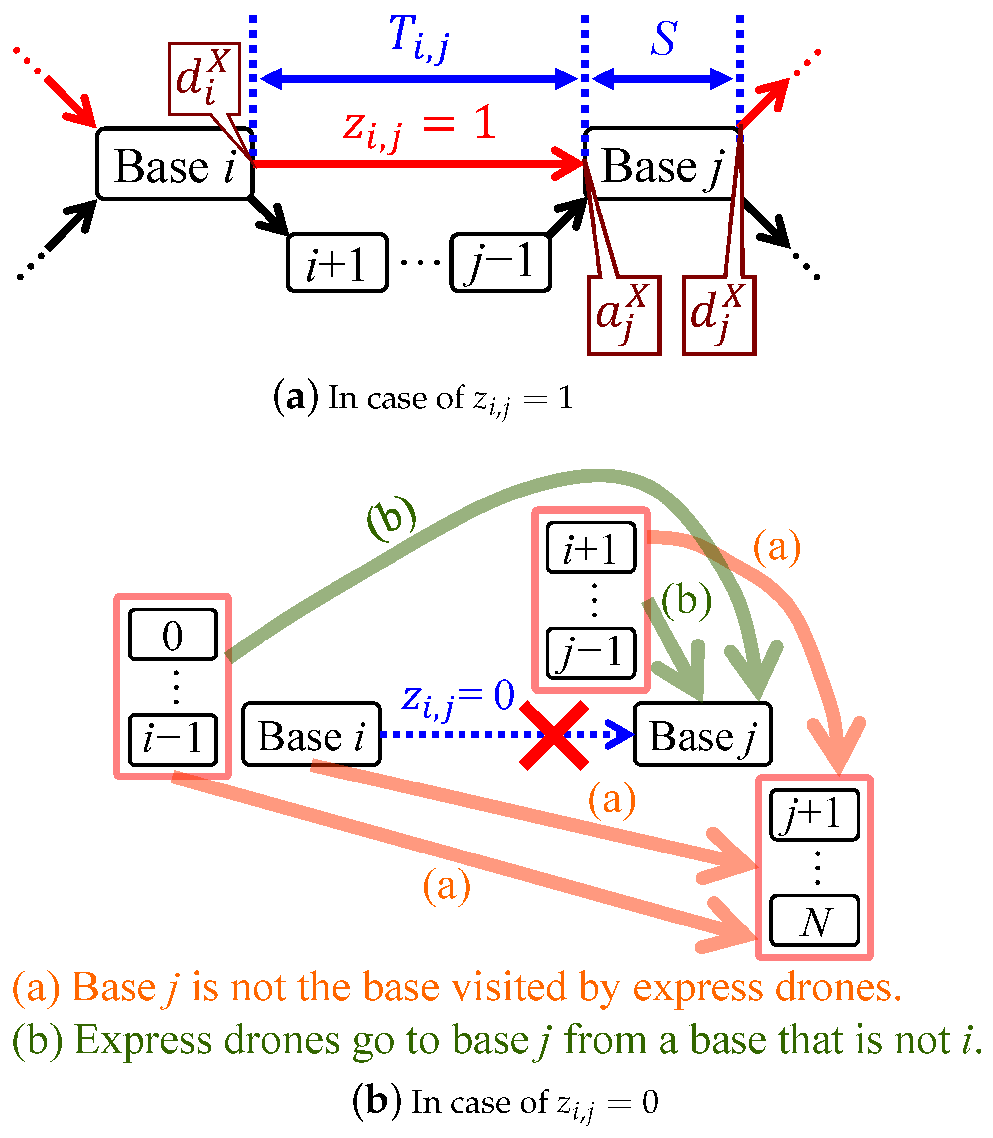
We consider the case in which transportation times can be formulated only in terms of the flight schedule of one lap of the drones ($j\le N$). Even if only a part of the section from base i to j is available for transportation by an express drone, the transportation time varies significantly. We divide the case into four groups according to whether bases i and j are visited by express drones and denote each transportation time by variables $t_{i,j}^{L,L},t_{i,j}^{L,X},t_{i,j}^{X,X},t_{i,j}^{X,L}$ ($i\in \mathcal{N},j\in {\overline{\overline{\mathcal{N}}}}_{i+1,N}$). The indices L and X in these variables are symbols for local and express drones, respectively. They also indicate which type of drone departs from base i and which type arrives at base j. For example, $t_{i,j}^{L,X}$ is the transportation time when a local drone departs from base i and an express drone arrives at base j. Note that ${\overline{\overline{\mathcal{N}}}}_{i+1,N}$ is ${\overline{\mathcal{N}}}_{i+1,N}$ when $i\ne 0$ and ${\overline{\mathcal{N}}}_{i+1,N-1}$ when $i=0$. The details of the four transportation times are described below.

Consider $t_{i,j}^{L,L}$ in the case in which both bases i and j are not visited by express drones ($x_i=x_j=0$). If multiple bases are visited by express drones between bases $i+1$ and $j-1$, it is possible for an express drone to transport packages a section along the way, which may be faster than a local drone transporting packages along the entire section from base i to j. Let $r_{i,j}^I$ be the base closest to i and $r_{i,j}^J$ be the base closest to j among the bases visited by express drones in the section from $i+1$ to $j-1$. In this case, the fastest transportation from base i to j can be achieved by a local drone transporting packages from base i to $r_{i,j}^I$, an express drone transporting packages from base $r_{i,j}^I$ to $r_{i,j}^J$, and a local drone transporting packages from base $r_{i,j}^J$ to j; that is, $r_{i,j}^I$ is the base for transferring packages from a local drone to an express drone and $r_{i,j}^J$ is the base for transferring packages from an express drone to a local drone. Let $u_{i,j}^I,u_{i,j}^J$ be the variables for the connections of local and express drones at bases $r_{i,j}^I,r_{i,j}^J$, respectively. $u_{i,j}^I$ represents the flight number of the local drone that connects to the first express drone at base $r_{i,j}^I$. $u_{i,j}^J$ represents the flight number of the local drone that the first express drone connects to at base $r_{i,j}^J$. $t_{i,j}^{L,L}(i\in \mathcal{N},j\in {\overline{\overline{\mathcal{N}}}}_{i+1,N})$ is expressed as the following equation using $u_{i,j}^I,u_{i,j}^J$:

$$t_{i,j}^{L,L}=(a_j^L+H_W·u_{i,j}^J)-(d_i^L+H_W·u_{i,j}^I).$$

(4)

The formulation of the variables $u_{i,j}^I,u_{i,j}^J,r_{i,j}^I,r_{i,j}^J$ is described in Section 4.3.

Consider $t_{i,j}^{L,X}$ in the case in which base i is not visited by express drones ($x_i=0$) and base j is visited by express drones ($x_j=1$). If more than one base is visited by express drones between $i+1$ and $j-1$, it is possible to transport packages from i to $r_{i,j}^I$ using a local drone and $r_{i,j}^I$ to j using an express drone, which may be faster. $t_{i,j}^{L,X}(i\in \mathcal{N},j\in {\overline{\overline{\mathcal{N}}}}_{i+1,N})$ is expressed as the following equation using $u_{i,j}^I$:

$$t_{i,j}^{L,X}=a_j^X-(d_i^L+H_W·u_{i,j}^I).$$

(5)

Consider $t_{i,j}^{X,X}$ in the case in which both base i and j are visited by express drones ($x_i=x_j=1$). In this case, $t_{i,j}^{X,X}(i\in \mathcal{N},j\in {\overline{\overline{\mathcal{N}}}}_{i+1,N})$ is expressed as follows because an express drone can transport packages along the entire section:

$$t_{i,j}^{X,X}=a_j^X-d_i^X.$$

(6)

Consider $t_{i,j}^{X,L}$ in the case in which base i is visited by express drones ($x_i=1$) and base j is not visited by express drones ($x_j=0$). If more than one base is visited by express drones between $i+1$ and $j-1$, it is possible to transport packages from i to $r_{i,j}^J$ using an express drone and $r_{i,j}^J$ to j using a local drone, which may be faster. $t_{i,j}^{X,L}(i\in \mathcal{N},j\in {\overline{\overline{\mathcal{N}}}}_{i+1,N})$ is expressed as the following equation using $u_{i,j}^J$:

$$t_{i,j}^{X,L}=(a_j^L+H_W·u_{i,j}^J)-d_i^X.$$

(7)

The transportation time $t_{i,j}^L$ ($i\in \mathcal{N},j\in {\overline{\overline{\mathcal{N}}}}_{i+1,N}$) is defined as the time required for a local drone to transport packages along the entire section from base i to j without transferring packages at intermediate bases and is expressed as the following equation:

$$t_{i,j}^L=a_j^L-d_i^L.$$

(8)

For transportation times $t_{i,j}^{L,L},t_{i,j}^{L,X},t_{i,j}^{X,L}$, if no base is visited by express drones between bases $i+1$ and $j-1$, or if there is one section from base i to j ($j-i=1$), packages cannot be transported by express drones. Furthermore, even if transportation by an express drone is possible, it is inefficient to use an express drone if express drones do not overtake local drones on the timetable. In such cases, the fastest transportation method is to use a local drone for the entire section. Therefore, it is necessary to compare $t_{i,j}^{L,L}$, $t_{i,j}^{L,X}$, and $t_{i,j}^{X,L}$ with $t_{i,j}^L$, and select the one with the smaller value to obtain the fastest transportation time for each section.

The transportation time between each base $t_{i,j}$ ($i\in \mathcal{N},j\in {\overline{\overline{\mathcal{N}}}}_{i+1,N}$) in the case of $j\le N$ can be expressed as follows:

$$\begin{array}{cc}\hfill t_{i,j}& =(1-x_i)(1-x_j)\left({\displaystyle \frac{H_W}{2}}+min\{t_{i,j}^{L,L},t_{i,j}^L\}\right)\hfill \\ \hfill & +(1-x_i)x_j\left({\displaystyle \frac{H_W}{2}}+min\{t_{i,j}^{L,X},t_{i,j}^L\}\right)\hfill \\ \hfill & +x_i·x_j\left({\displaystyle \frac{H_W}{4}}+t_{i,j}^{X,X}\right)\hfill \\ \hfill & +x_i(1-x_j)\left({\displaystyle \frac{H_W}{4}}+min\{t_{i,j}^{X,L},t_{i,j}^L\}\right).\hfill \end{array}$$

(9)

In the first half of each line of Equation (9), the case conditions for $t_{i,j}^{L,L},t_{i,j}^{L,X},t_{i,j}^{X,X}$, and $t_{i,j}^{X,L}$ are expressed as a product of $x_i$ and $x_j$. In the second half of the line, the fastest transportation times are obtained for each case, and the average waiting time $H_w/2$ or $H_w/4$ for packages to depart base i is added. The waiting time is $H_W/4$ for bases visited by express drones and $H_W/2$ for bases not visited. Note that $H_W/2,H_W/4$ may be decimals; hence, $t_{i,j}$ is a real-valued variable.

Next, we consider the transportation times for the case in which two laps of the flight schedule are required ($N+1\le j$). As described in Section 3, the departure times of the k-th local and express drones at base N (base 0) are $(k-1)H_w,(k-1)H_w+\eta$, respectively. Therefore, drones may stay at base N for a long time to adjust their time. In the case of a long dwell time, the orders of the arrival and departure of drones at base N do not necessarily coincide, as shown in Figure 7. Therefore, it is necessary to consider the possibility of a connection between a local drone and an express drone at base N.

First, we consider the transportation times from base N to j ($j\in {\overline{\mathcal{N}}}_{N+1,2N-2}$). We divide the case of the arrival of a local drone at base N and the case of the arrival of an express drone. In the former case, let the times required to reach base j be the variables ${\xi }_j^{L,L},{\xi }_j^{X,X},{\xi }_j^{X,L}$. The first of the upper indices of these variables indicates which type of drone departs from base N, and the second index indicates which type of drone arrives at base j. Now, we define a variable $v_j^I$ that represents the number of flights of the local drone connecting to the first express drone at each base. When $e=jmodN$, variables ${\xi }_j^{L,L},{\xi }_j^{X,X},{\xi }_j^{X,L}(j\in {\overline{\mathcal{N}}}_{N+1,2N-2})$ are expressed as follows:

$$\begin{array}{cc}\hfill {\xi }_j^{L,L}& =a_j^L-a_N^L,\hfill \end{array}$$

(10)

$$\begin{array}{cc}\hfill {\xi }_j^{X,X}& =(d_N^X-a_0^L+H_W·v_N^I)+t_{0,e}^{X,X},\hfill \end{array}$$

(11)

$$\begin{array}{cc}\hfill {\xi }_j^{X,L}& =(d_N^X-a_0^L+H_W·v_N^I)+t_{0,e}^{X,L}.\hfill \end{array}$$

(12)

Equations (10)–(12) include a dwell time at base N or a waiting time for a connection from a local drone to an express drone. Equation (10) represents the time required for a single local drone to reach base j without transferring packages at base N. Equation (11) represents the time required to transfer packages to an express drone at base N and for an express drone to transport them to base j. Equation (12) represents the transportation time for first transferring packages to an express drone at base N, then transferring packages to a local drone at one of the bases from $N+1$ to $j-1$, and finally reaching base j.

In the case of the arrival of an express drone at base N, let the variables ${\tau }_j^{X,X},{\tau }_j^{X,L},{\tau }_j^{L,L}$ denote the time required to reach base j. The meaning of the upper indices in these variables is the same as that of the variables ${\xi }_j^{L,L},{\xi }_j^{X,X},{\xi }_j^{X,L}$. Let $v_j^J$ be a variable representing that the first express drone connects to the ($v_j^J+1$)-th local drone at base $j(j\in {\overline{\mathcal{N}}}_{1,N})$ and $u_X$ be a variable representing the number of express drones that left base 0 between time 0 and the time the first express drone returns to base 0. ${\tau }_j^{X,X},{\tau }_j^{X,L},{\tau }_j^{L,L}(j\in {\overline{\mathcal{N}}}_{N+1,2N-2})$ are expressed as the following equations:

$$\begin{array}{cc}\hfill {\tau }_j^{X,X}& =(a_e^X+H_W·u_X)-a_N^X,\hfill \end{array}$$

(13)

$$\begin{array}{cc}\hfill {\tau }_j^{X,L}& =(d_N^X-a_N^X)+t_{0,e}^{X,L},\hfill \end{array}$$

(14)

$$\begin{array}{cc}\hfill {\tau }_j^{L,L}& =(d_0^L+H_W·v_N^J-a_N^X)+t_{0,e}^L.\hfill \end{array}$$

(15)

Equations (13)–(15) include a dwell time at base N or a waiting time for a connection from an express drone to a local drone, respectively. Equation (13) represents the time required for a single express drone to reach base j without transferring packages at base N. Equation (14) represents the time when packages are not transferred at base N, but are transferred to a local drone at one of the bases from $N+1$ to $j-1$, and then transferred to base j. Equation (15) represents the time required to transfer packages to a local drone at base N and then to base j using the local drone.

Next, we formulate the transportation times from base i to j ($i\in {\overline{\mathcal{N}}}_{2,N-1},j\in {\overline{\mathcal{N}}}_{N+1,i+N-1}$) using the transportation times from base N to j. The transportation times for the arrival of a local drone at base N are defined as the variables ${\xi }_{i,j}^{L,L},{\xi }_{i,j}^{L,\ast }$ and the transportation times for the arrival of an express drone at base N as the variables ${\tau }_{i,j}^{L,L},{\tau }_{i,j}^{L,\ast },{\tau }_{i,j}^{X,\ast },{\tau }_{i,j}^{X,L}$. The first of the upper indices of these variables indicates which type of drone departs from base i, and the second index indicates which type of drone reaches base j. * denotes whether the drone is an express drone (X) or local drone (L). From base i to N, packages are transported by a single local drone, and ${\xi }_{i,j}^{L,L},{\xi }_{i,j}^{L,\ast }(i\in {\overline{\mathcal{N}}}_{2,N-1},j\in {\overline{\mathcal{N}}}_{N+1,i+N-1})$ is expressed as the following equation:

$$\begin{array}{cc}\hfill {\xi }_{i,j}^{L,L}& =t_{i,N}^L+min\{{\xi }_j^{X,L},{\xi }_j^{L,L}\},\hfill \end{array}$$

(16)

$$\begin{array}{cc}\hfill {\xi }_{i,j}^{L,\ast }& =t_{i,N}^L+min\{{\xi }_j^{X,X},{\xi }_j^{L,L}\}.\hfill \end{array}$$

(17)

The first half of Equations (16) and (17) represents the transportation times from base i to N, and the second half is the transportation times from base N to j. In the second half of each equation, the transportation times are compared between transferring packages to an express drone at base N and not transferring packages to an express drone at base N, and the smaller value is selected. To indicate whether base j is visited by express drones, $x_j=0$ for expression (16), and $x_j=1$ for expression (17). Note that the expressions (16) and (17) are valid regardless of whether base i is visited by express drones. Next, we consider the scenario in which ${\tau }_{i,j}^{L,L},{\tau }_{i,j}^{L,\ast },{\tau }_{i,j}^{X,\ast },{\tau }_{i,j}^{X,L}(i\in {\overline{\mathcal{N}}}_{2,N-1},j\in {\overline{\mathcal{N}}}_{N+1,i+N-1})$. Two possible cases exist, one in which an express drone is used to transport packages from base i to N and the other in which packages are switched from a local drone to an express drone between bases $i+1$ and $N-1$. This is expressed as the following equation:

$$\begin{array}{cc}\hfill {\tau }_{i,j}^{L,L}& =t_{i,N}^{L,X}+min\{{\tau }_j^{X,L},{\tau }_j^{L,L}\}\hfill \end{array}$$

(18)

$$\begin{array}{cc}\hfill {\tau }_{i,j}^{L,\ast }& =t_{i,N}^{L,X}+min\{{\tau }_j^{X,X},{\tau }_j^{L,L}\}\hfill \end{array}$$

(19)

$$\begin{array}{cc}\hfill {\tau }_{i,j}^{X,\ast }& =t_{i,N}^{X,X}+min\{{\tau }_j^{X,X},{\tau }_j^{L,L}\}\hfill \end{array}$$

(20)

$$\begin{array}{cc}\hfill {\tau }_{i,j}^{X,L}& =t_{i,N}^{X,X}+min\{{\tau }_j^{X,L},{\tau }_j^{L,L}\}.\hfill \end{array}$$

(21)

The first half of Equations (18)–(21) represents the transportation times from base i to N, and the second half represents the transportation times from base N to j. In the second half of each equation, the transportation times are compared between the case where packages are transferred to a local drone at base N and the case where packages are not transferred, and the smaller value is selected. To indicate whether bases $i,j$ are visited by express drones, $x_i=x_j=0$ in Equation (18), $x_i=0,x_j=1$ in Equation (19), $x_i=x_j=1$ in Equation (20), and $x_i=1,x_j=0$ in Equation (21).

In the case of base $j\ge N+1$, each transportation time $t_{i,j}(i\in {\overline{\mathcal{N}}}_{2,N-1},j\in {\overline{\mathcal{N}}}_{N+1,i+N-1})$ between each base is expressed as follows:

$$\begin{array}{cc}\hfill t_{i,j}& =(1-x_i)(1-x_j)\left({\displaystyle \frac{H_W}{2}}+min\{{\tau }_{i,j}^{L,L},{\xi }_{i,j}^{L,L}\}\right)\hfill \\ \hfill & +(1-x_i)x_j\left({\displaystyle \frac{H_W}{2}}+min\{{\tau }_{i,j}^{L,\ast },{\xi }_{i,j}^{L,\ast }\}\right)\hfill \\ \hfill & +x_i·x_j\left({\displaystyle \frac{H_W}{4}}+min\{{\tau }_{i,j}^{X,\ast },{\xi }_{i,j}^{L,\ast }\}\right)\hfill \\ \hfill & +x_i(1-x_j)\left({\displaystyle \frac{H_W}{4}}+min\{{\tau }_{i,j}^{X,L},{\xi }_{i,j}^{L,L}\}\right).\hfill \end{array}$$

(22)

Equation (22) is constructed similarly to Equation (9), with $i,j$ divided into cases based on whether they are bases visited by express drones, and the fastest transportation time is obtained in each case. Equations (9) and (22) provide the fastest transportation times between all logistics bases. Note that some of the formulas up to equation (22) are non-linear due to products of variables or minimum value functions. Appendix A.1–Appendix A.3 describe how to transform these into linear expressions.

4.3. Constraints

We formulate the following three constraints. The first is constraints on the flight routes of express drones, which are formulated for the route ${\mathcal{P}}_X$. The second is constraints on the arrival and departure times of drones at each base $d_j^L,d_j^X,a_j^L,a_j^X$. We also formulate the arrival and departure times for the second lap of the flight. The third is constraints on the connections between local drones and express drones at each base. We formulate the variables $r_{i,j}^I,r_{i,j}^J,u_{i,j}^I,u_{i,j}^J,v_j^I,v_j^J$ as shown in Section 4.2. The following sections are divided into subsections for each matter.

4.3.1. Constraints on the Flight Route of Express Drones

We define a binary variable $z_{i,j}$ ($i\in \mathcal{N},j\in {\overline{\overline{\mathcal{N}}}}_{i+1,N}$) that is 1 if express drones visit base i and then base j, and 0 otherwise. The constraints on the construction of the route ${\mathcal{P}}_X$ are as follows:

$$\sum _{j\in {\overline{\mathcal{N}}}_{1,N-1}}{z}_{0,j}=\sum _{j\in {\overline{\mathcal{N}}}_{1,N-1}}{z}_{j,N}=1,$$

(23)

$$0\le \sum _{j\in {\overline{\mathcal{N}}}_{i+1,N}}{z}_{i,j}\le 1,0\le \sum _{j\in {\overline{\mathcal{N}}}_{0,i-1}}{z}_{j,i}\le 1(i\in {\overline{\mathcal{N}}}_{1,N-1}),$$

(24)

$$\sum _{j\in {\overline{\mathcal{N}}}_{i+1,N}}{z}_{i,j}=\sum _{j\in {\overline{\mathcal{N}}}_{0,i-1}}{z}_{j,i}(i\in {\overline{\mathcal{N}}}_{1,N-1}).$$

(25)

Equation (23) represents that the terminal point, base 0 (base N), is always the base visited by express drones. Equations (24) and (25) represent that each base other than the terminal point is or is not visited by express drones. Equations (23)–(25) construct a circular route ${\mathcal{P}}_X$ that connects the bases visited by express drones in a straight line, as shown in (Figure 4). Using $z_{i,j}$, the binary variable $x_i$ that represents the bases visited by express drones can be formulated as follows:

$$\sum _{j\in {\overline{\overline{\mathcal{N}}}}_{i+1,N}}{z}_{i,j}=x_i(i\in \mathcal{N}).$$

(26)

4.3.2. Constraints on the Arrival and Departure Times of Drones

We consider the constraints on the arrival and departure times of the first lap at each base. Let $T_{i,j}$ be a constant that represents the time required by drones from base i to j, S be a constant that represents the dwell time of drones at each base, and M be a sufficiently large positive number. The variables $d_j^L,d_j^X,a_j^L,a_j^X$ are expressed as follows:

$$d_0^L=0,a_j^L=d_{j-1}^L+T_{j-1,j}(j\in {\overline{\mathcal{N}}}_{1,N}),d_j^L=a_j^L+S(j\in {\overline{\mathcal{N}}}_{1,N-1}),$$

(27)

$$\begin{array}{cc}\hfill & d_0^X=\eta ,d_j^X=a_j^X+x_j·S(j\in {\overline{\mathcal{N}}}_{1,N-1}),\hfill \\ \hfill & d_i^X+T_{i,j}-M(1-z_{i,j})\le a_j^X\le d_i^X+T_{i,j}+M(1-z_{i,j})(i\in \mathcal{N},j\in {\overline{\overline{\mathcal{N}}}}_{i+1,N}).\hfill \end{array}$$

(28)

Equation (27) denotes the departure and arrival times of local drones flying along the route ${\mathcal{P}}_L$. Note that $d_j^L,a_j^L$ can be treated as constants because the departure time of the first drone at base 0, the time required between each base, and the flight interval of drones of the same type are all constants. Equation (28) denotes the arrival and departure times of express drones flying along the path ${\mathcal{P}}_X$. Equation (28) allows us to correctly calculate the arrival and departure times of express drones on the route ${\mathcal{P}}_X$ that connects the visited bases in a straight line and does not pass through other bases, regardless of which bases the express drones visit. For the third inequality in Equation (28), when $z_{i,j}=1$, $a_j^X=d_i^X+T_{i,j}$, which is the same as for local drones (Figure 8a). When $z_{i,j}=0$, M is a sufficiently large number; hence, $-M\le a_j^X\le M$. This means that the value of $a_j^X$ is undefined because express drones may not visit base j or may come to base j from a different base than base i (Figure 8b). Note that $\eta$ represents the headway between successive local and express drones at base 0, which is subject to the following two constraints, as described in Section 3:

$$\begin{array}{cc}\hfill & 0\le \eta \le H_W-I_C,\hfill \end{array}$$

(29)

$$\begin{array}{cc}\hfill & \eta =\beta ·I_C,\hfill \end{array}$$

(30)

where $I_C$ is a constant that represents the smallest increment in the timetable and $\beta$ is an integer variable greater than or equal to 0. Equation (30) is the constraint that $\eta$ must be a multiple of $I_C$.

Next, we consider the constraints on the departure and arrival times of the second round of flights. Note that when drones return to base 0 and start flying along their respective routes again, the departure times of local and express drones must be $(k-1)H_W$, $(k-1)H_W+\eta$ ($k\in \mathbb{N}$), respectively, and the variables $u_L,u_X$ are defined. $u_L$ (resp. $u_X$) represents the number of local drones (resp. express drones) that left base 0 between time 0 and the time the first local drone (resp. express drone) returns to base 0 and is ready to depart. The arrival and departure times of the second round are expressed as the following equation using $u_L,u_X$ and the arrival and departure times of the first round:

$$d_{j+N}^L=d_j^L+u_L·H_W,d_{j+N}^X=d_j^X+u_X·H_W(j\in \mathcal{N}),$$

(31)

$$a_{j+N}^L=a_j^L+u_L·H_W,a_{j+N}^X=a_j^X+u_X·H_W(j\in {\overline{\mathcal{N}}}_{1,N}).$$

(32)

The values of the variables $u_L,u_X$ are formally defined through the following constraints:

$$\begin{array}{cc}\hfill & S\le (d_0^L+u_L·H_W)-a_N^L\le S+H_W-I_C,\hfill \end{array}$$

(33)

$$\begin{array}{cc}\hfill & S\le (d_0^X+u_X·H_W)-a_N^X\le S+H_W-I_C.\hfill \end{array}$$

(34)

Equations (33) and (34) are the constraints on the dwell time that local drones and express drones stay at base 0 to adjust their times before starting the second round of the routes, respectively. Note that $u_L$ can also be treated as a constant because the arrival and departure times of the local drone at each base are constants.

The constraints on the bases visited by express drones during the first and second rounds of the flight route are given by

$$x_{j+N}=x_j(j\in \mathcal{N}).$$

(35)

Equation (35) is the constraint that the bases visited by express drones must be the same on the first and second rounds of the route.

4.3.3. Constraints on Connections Between Local and Express Drones

First, the variables $r_{i,j}^I,r_{i,j}^J(i\in {\overline{\mathcal{N}}}_{0,N-2},j\in {\overline{\overline{\mathcal{N}}}}_{i+2,N})$, which represent the base closest to i and the base closest to j among the bases visited by express drones between bases $i+1$ and $j-1$, are formulated as follows:

$$\begin{array}{cc}\hfill & r_{i,j}^I=min\{n\mid x_n=1,n\in {\overline{\mathcal{N}}}_{i+1,j-1}\},\hfill \end{array}$$

(36)

$$\begin{array}{cc}\hfill & r_{i,j}^J=max\{n\mid x_n=1,n\in {\overline{\mathcal{N}}}_{i+1,j-1}\},\hfill \end{array}$$

(37)

where ${\overline{\overline{\mathcal{N}}}}_{i+2,N}$ is ${\overline{\mathcal{N}}}_{i+2,N}$ when $i\ne 0$ and ${\overline{\mathcal{N}}}_{i+2,N-1}$ when $i=0$. $r_{i,j}^I,r_{i,j}^J$ are defined when there are at least two sections from base i to j ($j-i\ge 2$). Note that Equations (36) and (37) contain minimum value functions. The approach used to convert them to linear equations is described in the Appendix A.4.

Next, we formulate the variables $u_{i,j}^I,u_{i,j}^J$, which represent how many flights of local drones connect to the first express drone at base $r_{i,j}^I$ and how many flights of local drones connect from the first express drone at base $r_{i,j}^J$. The following is an example of the formulation of the variable $u_{i,j}^I$. We define a binary variable $y_{i,j}$ that is 1 if one or more bases are visited by express drones between bases $i+1$ and $j-1$, and 0 otherwise; a binary variable $y_{i,j,k}^I,y_{i,j,k}^J$ that is 0 or 1; and a sufficiently large number $M_S$ that satisfies $M_S\ll M$. $u_{i,j}^I,u_{i,j}^J(i\in {\overline{\mathcal{N}}}_{0,N-2},j\in {\overline{\overline{\mathcal{N}}}}_{i+2,N})$ are expressed as the following equations using these variables and the constant:

$$u_{i,j}^I=\left\{\begin{array}{cc}\sum _{k\in {\overline{\mathcal{N}}}_{i+1,j-1}}{v}_k^I·y_{i,j,k}^I\hfill & (j-i\ge 2)\hfill \\ 0\hfill & (j-i=1),\hfill \end{array}\right.$$

(38)

$$u_{i,j}^J=\left\{\begin{array}{cc}\sum _{k\in {\overline{\mathcal{N}}}_{i+1,j-1}}{v}_k^J·y_{i,j,k}^J+M_S(1-y_{i,j})\hfill & (j-i\ge 2)\hfill \\ M_S\hfill & (j-i=1).\hfill \end{array}\right.$$

(39)

The variable $y_{i,j,k}^I$ has the role of substituting the variable $v_k^I$ at base $r_{i,j}^I$ for $u_{i,j}^I$ for each base from $i+1$ to $j-1$. $y_{i,j,k}^J$ has the role of substituting $v_k^J$ at base $r_{i,j}^J$ for $u_{i,j}^J$. Furthermore, if no bases are visited by express drones between bases $i+1$ and $j-1$, the variables also have the roles of substituting 0 for $u_{i,j}^I$ and $M_S$ for $u_{i,j}^J$. Note that the case of one section from base i to j ($j-i=1$), $u_{i,j}^I,u_{i,j}^J$ is treated as the case where no base is visited by express drones between bases $i+1$ and $j-1$. Therefore, $u_{i,j}^I,u_{i,j}^J$ are divided into cases, as shown in Equations (38) and (39). Thus, $y_{i,j,k}^I,y_{i,j,k}^J$ ($i\in {\overline{\mathcal{N}}}_{0,N-2},j\in {\overline{\overline{\mathcal{N}}}}_{i+2,N},k\in {\overline{\mathcal{N}}}_{i+1,j-1}$) must satisfy the following constraints:

$$\begin{array}{cc}\hfill & r_{i,j}^I-M(1-y_{i,j})\le \sum _{k\in {\overline{\mathcal{N}}}_{i+1,j-1}}k·y_{i,j,k}^I\le r_{i,j}^I,\hfill \\ \hfill & r_{i,j}^J-M(1-y_{i,j})\le \sum _{k\in {\overline{\mathcal{N}}}_{i+1,j-1}}k·y_{i,j,k}^J\le r_{i,j}^J,\hfill \end{array}$$

(40)

$$\sum _{k\in {\overline{\mathcal{N}}}_{i+1,j-1}}{y}_{i,j,k}^I=y_{i,j},\sum _{k\in {\overline{\mathcal{N}}}_{i+1,j-1}}{y}_{i,j,k}^J=y_{i,j}.$$

(41)

$y_{i,j}$ is a binary variable that is 1 if one or more bases are visited by express drones between bases $i+1$ and $j-1$, and 0 otherwise. This is defined when there are at least two sections from base i to j. Thus, using the following constraint, $y_{i,j}(i\in {\overline{\mathcal{N}}}_{0,N-2},j\in {\overline{\overline{\mathcal{N}}}}_{i+2,N})$ can be bounded by the following inequalities:

$$x_k\le y_{i,j}\le \sum _{m\in {\overline{\mathcal{N}}}_{i+1,j-1}}{x}_m(k\in {\overline{\mathcal{N}}}_{i+1,j-1}).$$

(42)

We formulate constraints on the variables $v_j^I,v_j^J$ that represent how many flights of local drones connect to the first express drone and how many flights of local drones connect from the first express drone at each base. The connection is made in a minimum amount of time while allowing sufficient time to reload packages. In this study, the minimum time required for a connection is S, as is the dwell time at each base. Thus, in the case of a connection from the express drone to a local drone, the express drone connects with the local drone that first departs from base j after time S has elapsed from arrival time $a_j^X$, that is, after time $a_j^X+S$. The $v_j^J$ is a value that indicates how many flights this local drone is on. If the time between the arrival of the express drone at base j and the departure of the first local drone from base j is less than S, the express drone cannot connect with the local drone in question and connects with the local drone one flight later. Furthermore, in the case of a connection from a local drone to the express drone, the express drone connects to the local drone that last arrived at base j at a time S or more before the departure time $d_j^X$, that is, before time $d_j^X-S$. The $v_j^I$ is a value that indicates how many flights this local drone is on. If the time from the last arrival of a local drone at base j before departure time $d_j^X$ to time $d_j^X$ is less than S, the express drone cannot connect with the local drone in question and connects with the drone one flight ahead. Therefore, $v_j^I,v_j^J$ ($j\in {\overline{\mathcal{N}}}_{1,N}$) at each base can be bounded by the following inequalities:

$$\begin{array}{cc}\hfill & d_j^X-H_W+I_C\le (a_e^L+S)+H_W·v_j^I\le d_j^X,\hfill \end{array}$$

(43)

$$\begin{array}{cc}\hfill & a_j^X+S\le d_e^L+H_W·v_j^J\le (a_j^X+S)+H_W-I_C,\hfill \end{array}$$

(44)

where $e=jmodN$.

5. Approximate Solution Method for the MILP

This section first outlines the overall approach to approximating the solution of the proposed MILP in Section 5.1. We then describe the first step of selecting the bases to visit based on the number of packages and the layout of the bases in Section 5.2. Section 5.3 describes the second step of selecting bases to visit based on base adjacencies.

5.1. Outline

In this study, we propose a solution method to reduce the computational cost by fixing the value of the MILP decision variable $x_j$ and compute an approximate solution by solving the MILP repeatedly. By fixing the value of the binary variable $x_j(j\in \mathcal{N})$, which represents the bases visited by express drones, the only decision variable of the MILP is $\eta$ (the headway between a local drone and an express drone at base 0). Thus, the computational cost is greatly reduced. In the approximate solution method, the MILP is first solved by assuming that only one of the bases other than base 0 is visited by express drones, and then the optimal value of the objective function (Equation (3)) is obtained. The number of visited bases is then increased one at a time, and the optimal value is obtained for each increase. By repeating these processes until the optimal value is no longer decreasing, an approximate solution of the MILP is obtained. Such a solution method is based on the idea of the greedy method. The MILP computation is performed multiple times, but each time the computational cost is small; hence, the solution is obtained with less computational cost than the exact solution method of MILP.

The decision as to whether each base is to be visited by express drones is based on the number of packages handled at each base and the layout of the bases. The larger the number of packages, the more the base should be a visited base, and the more remote a base is from other bases, the less appropriate it is as a visited base. For example, in the case of the layout of the bases shown in Figure 9, base 2 is far from the other bases (bases 1 and 3) and should not be a visited base. If such a base is used as a visited base, the flight time per route of an express drone increases and transportation efficiency decreases.

In the approximate solution method, the approximate solution of MILP is obtained in two steps to determine the bases visited by express drones based on multiple guidelines. In the first step, the visited bases are determined from two perspectives: the number of packages at each base and the layout of all bases. In the second step, the visited bases are added based solely on the distance from each base to the adjacent base without considering the number of packages. The longer the distance to the adjacent base, the longer the flight time to this base; thus, such a base and its adjacent bases are appropriate visited bases. The first step is described in Section 5.2, and the second step is described in Section 5.3.

5.2. First Step: Determination of Visited Bases Based on the Number of Packages and the Layout of the Bases

The more packages handled at a base and the further away from other bases, the more appropriate it is as a base visited by express drones. Therefore, we define a constant $P_j(j\in \mathcal{N})$ that represents the number of packages handled at each base, the coordinates ${\mathbf{\chi }}_j(j\in \mathcal{N})$ of each base, and the distance $D_j^G$ ($j\in \mathcal{N}\backslash \left\{0\right\}$) from each base to the center of gravity. $D_j^G$ is given by the following equation:

$$D_j^G=∥{\mathbf{\chi }}_j-{\displaystyle \frac{1}{N}}\sum _{n\in \mathcal{N}}{\mathbf{\chi }}_n∥,$$

(45)

where $\parallel ·\parallel$ is the Euclidean distance and $\left({\sum }_{n\in \mathcal{N}}{\mathbf{\chi }}_n\right)/N$ are the coordinates of the center of gravity of the base. The coordinates of the center of gravity are calculated including the coordinates of base 0. The indicator ${\rho }_j(j\in \mathcal{N}\backslash \left\{0\right\})$, which evaluates whether each base is an appropriate visited base, is given by the following equation:

$${\rho }_j={\displaystyle \frac{P_j}{{\left(D_j^G\right)}^2}}.$$

(46)

Because base 0 is always visited by the express drone, ${\rho }_0$ is not included in the calculation. The appropriateness ${\rho }_j$ increases as the number of packages $P_j$ increases and the distance to the center of gravity $D_j^G$ decreases. This allows express drones to focus on the base with a large number of packages while minimizing the increase in the time required for one round of the route.

The first step of the approximate solution method is shown in Algorithm 1.

Algorithm 1 Approximate solution: first processing step

Input:  $\{{\rho }_1,{\rho }_2,\cdots ,{\rho }_{N-2},{\rho }_{N-1}\},\mathcal{N}$ Output:  ${\mathbf{x}}^{\mathrm{out}1}=(x_0^{\mathrm{out}1},x_1^{\mathrm{out}1},\cdots ,x_{\left|\mathcal{N}\right|-2}^{\mathrm{out}1},x_{\left|\mathcal{N}\right|-1}^{\mathrm{out}1})$ 1: $\mathbf{x}=(x_0,x_1,\cdots ,x_{\left|\mathcal{N}\right|-2},x_{\left|\mathcal{N}\right|-1})\leftarrow (1,0,\cdots ,0,0)$ 2: $\mathcal{J}\leftarrow \mathcal{N}\backslash \left\{0\right\},k\leftarrow \underset{j\in \mathcal{J}}{\arg \max }\left\{{\rho }_j\right\},x_k\leftarrow 1$ 3: opt_current ← Solve_MILP($\mathbf{x}$),    $\mathcal{J}\leftarrow \mathcal{J}\backslash \left\{k\right\}$ 4: while$\mathcal{J}\ne \varphi$do 5:    $k\leftarrow \underset{j\in \mathcal{J}}{\arg \max }\left\{{\rho }_j\right\}$,   $x_k\leftarrow 1$,   $\mathcal{J}\leftarrow \mathcal{J}\backslash \left\{k\right\}$ 6:    opt_temp ← Solve_MILP($\mathbf{x}$) 7:    if opt_temp < opt_current then 8:      opt_current ← opt_temp 9:    else 10:      $x_k\leftarrow 0$ 11:      break 12:    end if 13: end while 14: ${\mathbf{x}}^{\mathrm{out}1}\leftarrow \mathbf{x}$ 15: return ${\mathbf{x}}^{\mathrm{out}1}$

Algorithm 1 takes as input the set of bases $\mathcal{N}$ and the set of appropriateness values $\{{\rho }_1,{\rho }_2,\cdots ,{\rho }_{N-1}\}$. The output is the optimal arrangement of the bases visited by express drones in the first step ${\mathbf{x}}^{\mathrm{out}1}$. First, initialize the arrangement $\mathbf{x}$ on the first and second lines. Let $x_0=1,x_k=1(k=\underset{j\in \mathcal{J}}{\arg \max }\left\{{\rho }_j\right\})$. The other $x_i$ ($i\in \mathcal{N}\backslash \{0,k\}$) are assumed to be $x_i=0$ so that base 0 and the base with the largest appropriateness ${\rho }_j$ are the visited bases. Note that $\mathcal{J}$ is the auxiliary set of $\mathcal{N}$ excluding base 0. On the third line, the optimal value of the objective function of the MILP in the case of arrangement $\mathbf{x}$ is obtained using the function Solve_MILP and substituted into opt_current. Furthermore, base k is excluded from $\mathcal{J}$. From line 4 to line 13, the processes are repeated until $\mathcal{J}$ becomes an empty set $\varphi$ or no arrangement below opt_current is found. Each time the processes are repeated, the visited bases are added individually in the order of the bases with the largest appropriateness, and the optimal value opt_temp for arrangement $\mathbf{x}$ after the addition is obtained using the Solve_MILP function.

5.3. Second Step: Determination of the Visited Bases Based on the Adjacencies of Bases

In the second step, regardless of the number of packages, bases to be visited by express drones are added based on the adjacencies from each base to the bases on both sides. Specifically, if base $j-1,j+1$ on both sides of base j are further from the center of gravity than base j, then base j is an appropriate visited base. For example, base j in Figure 10 corresponds to this case.

To add such bases to visited bases, we define the appropriateness ${\alpha }_j(j\in \mathcal{N}\backslash \left\{0\right\})$ based on the adjacency relationship using the following equation:

$${\alpha }_j=\left(D_{j-1}^G-D_j^G\right)+\left(D_{j+1}^G-D_j^G\right).$$

(47)

Because base 0 is always visited by an express drone, ${\alpha }_0$ is not included in the calculation. The larger the value of ${\alpha }_j$, the closer base j is to the center of gravity compared with adjacent base $j-1,j+1$. Additionally, ${\alpha }_j$ is large when one of bases $j-1,j+1$ is far from the center of gravity and the other is closer to the center of gravity than base j. If ${\alpha }_j$ is negative, this indicates that base j is not an appropriate visited base because either or both of bases $j-1,j+1$ are definitely closer to the center of gravity than base j. Furthermore, even if ${\alpha }_j$ is positive, as mentioned above, it is possible that one of bases $j-1,j+1$ is closer to the center of gravity than base j; that is, the appropriateness of visited bases based on adjacencies does not necessarily follow the order of magnitude of ${\alpha }_j$. Therefore, let $\overline{\alpha }$ be the average of ${\alpha }_j$ ($j\in \mathcal{N}\backslash \left\{0\right\}$), where ${\alpha }_j$ is greater than or equal to $\overline{\alpha }$ (${\alpha }_j\ge \overline{\alpha }$) and greater than or equal to 0 (${\alpha }_j\ge 0$). Then base j is a candidate for a visited base. $\overline{\alpha }$ is obtained using the following equation:

$$\overline{\alpha }={\displaystyle \frac{1}{N-1}}\sum _{j\in \mathcal{N}\backslash \left\{0\right\}}{\alpha }_j.$$

(48)

Let ${\mathcal{N}}^{\sec }$ be the set of candidate visited bases in the second step, defined by the following equation:

$${\mathcal{N}}^{\sec }=\{j\in \mathcal{N}\backslash \left\{0\right\}\mid {\alpha }_j\ge \overline{\alpha },{\alpha }_j\ge 0,x_j^{\mathrm{out}1}=0\}.$$

(49)

The bases whose appropriateness ${\alpha }_j$ is greater than or equal to $\overline{\alpha }$ and also greater than or equal to 0, and which were not visited in the first step ($x_j^{\mathrm{out}1}=0$), are candidates for visited bases in the second step. In the second step, the bases selected as candidates are not ranked in the same way as in the first step.

The second step of the approximate solution method is shown in Algorithm 2.

Algorithm 2 Approximate solution: second processing step

Input:  ${\mathcal{N}}^{\sec },\mathcal{N},{\mathbf{x}}^{\mathrm{out}1}$ Output:  ${\mathbf{x}}^{\mathrm{out}2}=(x_0^{\mathrm{out}2},x_1^{\mathrm{out}2},\cdots ,x_{\left|\mathcal{N}\right|-2}^{\mathrm{out}2},x_{\left|\mathcal{N}\right|-1}^{\mathrm{out}2})$ 1: $\mathbf{x}=(x_0,x_1,\cdots ,x_{\left|\mathcal{N}\right|-2},x_{\left|\mathcal{N}\right|-1})\leftarrow {\mathbf{x}}^{\mathrm{out}1}$ 2: opt_current ← Solve_MILP(${\mathbf{x}}^{\mathrm{out}1}$),   $\mathcal{S}\leftarrow {\mathcal{N}}^{\sec }$ 3: while  $\mathcal{S}\ne \varphi$  do 4:    temp1 ← NULL,   num ← NULL,    $\mathcal{J}\leftarrow \mathcal{S}$ 5:    while $\mathcal{J}\ne \varphi$ do 6:      $k\leftarrow min\{j\mid j\in \mathcal{J}\},\mathcal{J}\leftarrow \mathcal{J}\backslash \left\{k\right\}$ 7:      $x_k\leftarrow 1$,   temp2 ← Solve_MILP($\mathbf{x}$) 8:      if (temp1 = NULL) or (temp2 < temp1) then 9:         temp1 ← temp2,    num $\leftarrow k$ 10:     end if 11:      $x_k\leftarrow 0$ 12:    end while 13:    if (temp1 ≠ NULL) and (temp1 < opt_current) then 14:      opt_current ← temp1,   $x_{\mathrm{num}}\leftarrow 1,\mathcal{S}\leftarrow \mathcal{S}\backslash \left\{\mathrm{num}\right\}$ 15:    else 16:      break 17:    end if 18: end while 19: ${\mathbf{x}}^{\mathrm{out}2}\leftarrow \mathbf{x}$ 20: return ${\mathbf{x}}^{\mathrm{out}2}$

Algorithm 2 takes as input the set of bases $\mathcal{N}$, the set of candidates for visited bases ${\mathcal{N}}^{\sec }$, and the arrangement of the visited bases in the first step ${\mathbf{x}}^{\mathrm{out}1}$. On the first line, $\mathbf{x}$ is initialized with the arrangement in the first step. On the second line, opt_current is initialized with the optimal value of the objective function for the arrangement in the first step placement and the auxiliary set $\mathcal{S}$ is initialized with ${\mathcal{N}}^{\sec }$. Then, the optimal value of each base in the candidate set $\mathcal{S}$ is obtained when each base is added to the visited bases individually, and the number of the candidate base when the optimal value is minimized is obtained as num (lines 5 to 12). When base-num is added to the visited bases, if the optimal value is less than the value of opt_current, opt_current is updated and base-num is added again to the visited bases (line 14). Furthermore, base-num is excluded from the set $\mathcal{S}$ and the same processes (lines 3–18) are repeated. If the optimal value is greater than or equal to the value of opt_current, the algorithm outputs the arrangement of the visited bases at that time as ${\mathbf{x}}^{\mathrm{out}2}$ without adding bases-num, and stops. The arrangement ${\mathbf{x}}^{\mathrm{out}2}$ is the approximate solution in the proposed solution method.

6. Performance Evaluation

We evaluated the performance of the proposed method by conducting experiments with and without regularity in the layout of logistics bases. In the former experiment, we set the number of bases to the extent that a computer can solve the MILP using the exact solution method in a realistic amount of time, and demonstrated that the bases visited by express drones were determined according to the appropriateness shown in Equations (46) and (47). In the latter experiment, we changed the number of logistics bases from a small number to a large number. In a scenario with a few logistics bases, we solved the MILP using both the exact and approximate solution methods, and demonstrated that the approximate solution method computed a solution close to the exact solution in a short time. The computer used in the experiments had an AMD EPYC 7443P CPU with a clock frequency of 1.5 GHz, 24 cores, and 528 GB of RAM. We used mathematical optimization software IBM CPLEX [30] on the computer to solve the MILP.

6.1. Experiment 1: The Case of a Regular Layout of Logistics Bases

We evaluate the performance of the proposed scheduling method in a simplified and controlled environment where logistics bases are arranged in a regular layout.

6.1.1. Setting of Experiment 1

In this experiment, we evaluated the performance of the proposed method under the assumption that logistics bases were located regularly, as shown in Figure 11. In this experiment, the number of bases was always eight ($N=8$). The proposed method in this experiment was the method used to transport packages by obtaining an optimal solution of the MILP without using the approximate solution method.

In Figure 11, the circles are the locations of the bases, the number in each circle is the base number, and the blue arrows make up the flight route of local drones ${\mathcal{P}}_L$. As shown in Figure 11, the size of one square in the coordinate plane is $100\times 100$. In Figure 11, the bases are equally spaced on the circumference of a circle of radius 500 centered at the origin of the coordinate plane, and the coordinates of base 0 (the terminal point) are (0, 500).

In this experiment, the location of one of the bases was moved from the origin of the coordinate plane along the direction toward the outside of the circle. As an example, the movement of base 2 is shown in Figure 12. As shown in the figure, the base was moved along a straight line connecting the origin and the base to be moved, and the shape of the route ${\mathcal{P}}_L$ changed as the base was moved. The bases were moved to four locations at distances of 0, 1000, 1500, and 2000 from the origin. All other bases except for base 2 were moved in the same manner, but only one base was moved at a time, and all other bases were fixed on the circumference. Note that base 0 was not moved because it was the terminal point.

Through these experiments, we examined how a change to the location of one of the bases affected the optimal solution (i.e., the base visited by express drones) and the optimal value of the MILP.

In this experiment, the number of packages handled at each base $P_j(j\in \mathcal{N})$ was determined as shown in

Table 3. Number of packages handled at each base ($P_j$).

	Base Number
	0	1	2	3	4	5	6	7
Number of packages	1000	800	700	400	900	100	300	200

. In all experiments conducted in this section, $P_j$ was fixed at the value in Table 3.

The values in Table 3 were converted to the number of packages transported between each base $W_{i,j}$ ($i\in \mathcal{N},j\in {\overline{\mathcal{N}}}_{i+1,i+N-1}$) using the following equation:

$$W_{i,j}=P_i·{\displaystyle \frac{P_j}{{\sum }_{n\in \mathcal{N}\backslash \left\{i\right\}}{P}_n}}.$$

(50)

On the right-hand side of Equation (50), when $j\ge N$, the value of $jmodN$ was taken as j. As described in Section 3, the unit of $W_{i,j}$ was not defined because the upper limit of a drone’s package capacity was sufficiently large.

The values of each parameter in the experiment are described as follows: The headway $H_W$ for each drone of the same type was 600 s; the dwell time by drones at each base other than base 0 (the minimum time required for drones to connect) S was 90 s; and the smallest increment in the timetable $I_C$ was 10 s. The time $T_{i,j}(i\in \mathcal{N},j\in {\overline{\overline{\mathcal{N}}}}_{i+1,N})$ required for a drone to fly in a straight line between each base was set using the following two equations:

$$T_{i,j}^{\ast }=⌈{\displaystyle \frac{\left|\right|{\mathbf{\chi }}_i-{\mathbf{\chi }}_j\left|\right|}{v_{\mathrm{drone}}}}⌉(i\in \mathcal{N},j\in {\overline{\overline{\mathcal{N}}}}_{i+1,N}),$$

(51)

$$T_{i,j}=\left\{\begin{array}{cc}{T}_{i,j}^{\ast }\hfill & (T_{i,j}^{\ast }mod{I}_C=0)\hfill \\ T_{i,j}^{\ast }+(I_C-T_{i,j}^{\ast }mod{I}_C)\hfill & (T_{i,j}^{\ast }mod{I}_C\ne 0),\hfill \end{array}\right.$$

(52)

where $\lceil ·\rceil$ is the ceiling function, $v_{\mathrm{drone}}$ is the drone’s flight speed, and $v_{\mathrm{drone}}=1$ in the experiment. However, $T_{i,j}$ must be a multiple of $I_C$. Because $I_C=10$ s in the experiment, if $T_{i,j}^{\ast }$ was not divisible by 10, it was rounded up to a multiple of 10 in Equation (52) and then substituted for $T_{i,j}$. The unit of $T_{i,j}$ is seconds.

We also present the results of the only local drones (OLD) and division by two types of drones (DTD) methods for a performance comparison with the proposed method. The details of each method are below.

• OLD method: For this method, only local drones are flown along the route ${\mathcal{P}}_L$ without considering the number of packages at each base. The number of drone flights departing from base 0 during $H_W=600$ s is the same as that in the proposed method. In the proposed method, one local drone and one express drone depart during $H_W$; hence, in the OLD method, two local drones depart during $H_W$. Because all drones are equally spaced, the headway for this method is $H_W/2=300$ s. By comparing the proposed method with such a method, we confirmed the effectiveness of express drones frequently visiting some bases in the proposed method.
• DTD method: In this method, two types of drones divide the responsibility of visiting bases. The two types of drones visit bases that are different from each other. One type of drone visits the bases visited by express drones in the proposed method, and the other type of drone visits the other bases. For consistency with the proposed method, we refer to the former type as an express drone and the latter type as a local drone. Both types of drones visit base 0 (the terminal point). Both types of drones depart from base 0 simultaneously with a headway $H_W=600$ s. By comparing the proposed method with such a method, we confirmed the validity of the proposed method in which local drones also visit the bases visited by express drones.

The performance indicator is the average transportation time per unit of package $\overline{T}$. $\overline{T}$ is obtained using the following equation, using the fastest transportation time $T_{i,j}$ between each base:

$$\overline{T}={\displaystyle \frac{{\sum }_{i\in \mathcal{N}}{\sum }_{j\in {\overline{\mathcal{N}}}_{i+1,i+N-1}}{W}_{i,j}·t_{i,j}}{{\sum }_{i\in \mathcal{N}}{\sum }_{j\in {\overline{\mathcal{N}}}_{i+1,i+N-1}}{W}_{i,j}}}.$$

(53)

The denominator of Equation (53) is the total number of all packages to be transported. The numerator is the total transportation times, which is the optimal value of the objective function of the MILP in the proposed method.

6.1.2. Evaluation Result: When All Bases Were Located on the Circumference

Figure 13 shows flight schedules of drones calculated by the proposed method and the two comparison methods when the layout of the bases is as shown in Figure 11, that is, when all eight bases were located on the circumference. In Figure 13, flight schedules of drones from the first to the fifth flight in one round of the routes are shown. The black dashed lines in the figure show the flight schedule of local drones, and the red solid lines show the flight schedule of express drones. Note that base number 8 on the vertical axis represents the terminal point, that is, base 0. Figure 13a shows that, in the proposed method, express drones visited bases 0, 1, 2, and 4. Therefore, Figure 13c, which is the result of the DTD method, shows that express drones visited bases 0, 1, 2, and 4, and local drones visited bases 0, 3, 5, 6, and 7. The headway $\eta$ of drones in the proposed method was 240 s.

Table 4. Average transportation time per unit of package $\overline{T}$ (experimental conditions: Figure 11 and Table 3).

	Proposal	OLD	DTD
$\overline{T}$ [s]	1715.5	1993.5	2235.5

shows the average transportation time $\overline{T}$ for each method in the experiment when the layout of the bases is as shown in Figure 11. Table 4 shows that the proposed method was an efficient method for transporting packages because $\overline{T}$ of the proposed method was the smallest. Furthermore, we confirmed the effectiveness of frequently visiting some bases for transportation and the validity of local drones also visiting bases visited by express drones.

6.1.3. Evaluation Result: When One Base Was Moved

Table 5. Bases visited by express drones (optimal solutions of MILP).

	Base Number
Base to Be Moved (Distance from the Origin)	0	1	2	3	4	5	6	7
Base 1 (0)	•	•			•
Base 1 (1000)	•		•		•
Base 1 (1500)	•		•		•
Base 1 (2000)	•		•	•	•
Base 2 (0)	•		•		•
Base 2 (1000)	•	•		•	•
Base 2 (1500)	•	•		•	•
Base 2 (2000)	•	•		•	•
Base 3 (0)	•	•		•
Base 3 (1000)	•	•	•		•
Base 3 (1500)	•	•	•		•
Base 3 (2000)	•	•	•		•
Base 4 (0)	•	•			•
Base 4 (1000)	•	•	•			•
Base 4 (1500)	•	•	•	•			•
Base 4 (2000)	•	•	•	•		•
Base 5 (0)	•	•	•			•
Base 5 (1000)	•	•	•		•
Base 5 (1500)	•	•	•		•		•
Base 5 (2000)	•	•			•		•
Base 6 (0)	•	•	•				•
Base 6 (1000)	•	•	•		•
Base 6 (1500)	•	•	•		•
Base 6 (2000)	•	•			•			•
Base 7 (0)	•	•	•		•			•
Base 7 (1000)	•	•	•		•
Base 7 (1500)	•	•	•		•		•
Base 7 (2000)	•	•			•		•

shows the optimal solutions of the MILP for the case where the location of one base was changed. The black circled bases are those visited by express drones.

Table 5 shows that the bases visited by express drones were determined by the number of packages and the distance from the center of gravity of each base, roughly following the magnitude of the appropriateness ${\rho }_j$ of Equation (46). Furthermore, the appropriateness ${\alpha }_j$ of Equation (47) was also important because bases on either side of a base located far from the center of gravity were almost always visited bases.

Figure 14 shows the change in the average transportation time $\overline{T}$ for each method as each base was moved. The horizontal axis of these graphs represents the distance between the base to be moved and the origin, and the vertical axis represents $\overline{T}$. $\overline{T}$ of the proposed method was the smallest, as shown in both graphs in Figure 14. Furthermore, the performance difference between the proposed method and the compared method was larger for bases 5, 6, and 7, which were the bases with the smallest number of packages as they are moved further away from the origin. Therefore, the proposed method was particularly effective when bases with a small number of packages were located far from the origin.

6.2. Experiment 2: The Case of an Irregular Layout of Logistics Bases

To evaluate the performance of the proposed method under more realistic conditions, we conducted an experiment assuming an irregular spatial layout of logistics bases.

6.2.1. Setting of Experiment 2

We conducted experiments assuming that there was no regularity in the layout of logistics bases in the real world. Specifically, we considered scenarios in which there were N logistics bases within a square region of $4000\times 4000$ centered at the origin. We assumed that the number of bases N was eight: 6, 7, 8, 9, 12, 16, 20, and 24. The coordinates of base 0 were ${\mathbf{\chi }}_0=(0,1000)$, and the coordinates of the other bases ${\mathbf{\chi }}_j(j\in \mathcal{N}\backslash \left\{0\right\})$ were $(100{ϵ}_j^x,100{ϵ}_j^y)$. Note that ${ϵ}_j^x,{ϵ}_j^y$ were uniform random numbers that were integer values from $-20$ to 20. Furthermore, the number of packages handled at base 0 was $P_0=2000$, and the number of packages at the other bases $P_j(j\in \mathcal{N}\backslash \left\{0\right\})$ was assigned randomly from among $\{100,200,\dots ,1800,1900\}$. For the conversion from $P_j$ to $W_{i,j}$, we used Equation (50), as in Experiment 1 shown in Section 6.1. We set the other parameters to the same values as in Experiment 1.

Local drones flew along the shortest route, visiting each base once. Because such a flight route can be formulated as integer linear programming (ILP) for the traveling salesman problem, the route was obtained by solving ILP. Let ${\mathcal{P}}_L$ be the route obtained by ILP. Number the bases from 1 to $N-1$, starting from the first base visited by a local drone departing from base 0. Figure 15 shows an example when the number of bases was eight.

We conducted experiments and compared the performance of four methods: cases in which the approximate solution method was not used in the computation of the proposed MILP and cases in which it was used, and the two comparison methods described in Experiment 1. To distinguish the proposed methods, we refer to them as “Proposal (MILP)” when the exact solution method was used and “Proposal (Approximate)” when the approximate solution method was used. Details of the OLD and DTD methods, which are comparison methods, are provided in Section 6.1.

The performance indicator is the mean value $E\left[\overline{T}\right]$ of 10 average transportation times $\overline{T}$; that is, for each N, we conducted 10 experiments, changing the layout of bases and the number of packages at each base. We describe the method for calculating the average transportation time in Section 6.1.

6.2.2. Evaluation Result

First, we show the results for the case in which the layout of logistics bases is as shown in Figure 15 and the number of packages at each base is as shown in

Table 6. Number of packages at each base in the flight schedules shown in this section ($P_j$).

	Base Number
	0	1	2	3	4	5	6	7
Number of packages	2000	1500	1800	300	800	1000	1300	500

.

Table 7. Bases visited by express drones (experimental conditions: Figure 15 and Table 6).

	Base Number
	0	1	2	3	4	5	6	7
Proposal (MILP)	•	•			•
Proposal (Approximate)	•	•			•

shows which bases were visited by express drones for Proposal (MILP) and Proposal (Approximate), respectively. The black circles indicate the visited bases.

From Table 7, the visited bases of Proposal (MILP) and Proposal (Approximate) were consistent. Furthermore, from Figure 15 and Table 6, the bases visited by express drones were those with a large number of packages located near the center of gravity.

The flight schedules calculated by each method in the experiments in Figure 15 and Table 6 are shown in Figure 16. Figure 16 shows the flight schedules for the first to third flights of local drones and the first to 15th flights of express drones for one round of the routes. The red and black lines represent the flight schedules of the express and local drones, respectively. Figure 16a shows that the results of Proposal (MILP) and Proposal (Approximate) were the same. In the flight schedules of the DTD method (Figure 16c), express drones visited bases 0, 1, and 4, and local drones visited bases 0, 2, 3, 5, 6, and 7. The headway $\eta$ of drones in the proposed method was 460 s.

Table 8. Average transportation times $\overline{T}$ (experimental conditions: Figure 15 and Table 6).

	Proposal (MILP, Approximate)	OLD Method	DTD Method
$\overline{T}$ [s]	2926.3	5267.1	4659.3

shows the average transportation time $\overline{T}$ for each method in the experiment in Figure 15 and Table 6. The values of $\overline{T}$ were also the same for Proposal (MILP) and Proposal (Approximate). Table 8 shows that the proposed method had the smallest $\overline{T}$, which indicates that the proposed method was an efficient method for transporting packages.

Figure 17 shows the change in the mean value $E\left[\overline{T}\right]$ for each method as the number of bases N increased. The horizontal axis of the figure represents N, and the vertical axis represents $E\left[\overline{T}\right]$. Figure 17 shows that $E\left[\overline{T}\right]$ of the proposed method was the smallest. Proposal (MILP) could not complete the computation within 3 h when the number of bases exceeded 9. In the range of N from 6 to 9, $E\left[\overline{T}\right]$ of Proposal (Approximate) was slightly larger than that of Proposal (MILP), but almost identical. Therefore, it was possible to compute a solution that was almost equal to the exact solution using the approximate solution method. Furthermore, $E\left[\overline{T}\right]$ of Proposal (Approximate) was smaller than those of the OLD and DTD methods in the range of N from 12 to 24. These results indicate that Proposal (Approximate) was an efficient method of transporting packages, even when the number of bases was large.

Finally, the computation time required to solve the MILP using Proposal (MILP) and Proposal (Approximiate) is shown in

Table 9. Average computation time [s].

	Number of Bases
	$\mathit{N}=\mathbf{6}$	$\mathit{N}=\mathbf{9}$	$\mathit{N}=\mathbf{16}$	$\mathit{N}=\mathbf{24}$
Proposal (MILP)	0.564	38.6	—	—
Proposal (Approximate)	0.353	0.838	19.7	352

. The values in the table are means of the computation time over 10 experiments. The computation time of Proposal (Approximate) includes the time required to obtain the appropriateness for the bases visited by express drones and the candidate visited bases based on Equations (46) and (47). In Proposal (MILP), when the number of bases N exceeded 9, the solution could not be computed, even after more than 3 h from the start of the computation. By contrast, Proposal (Approximate) completed the computation in a very short time. This result indicates that Proposal (Approximate) significantly reduced the computational cost.

7. Conclusions

In this study, we considered a method to calculate flight schedules for drones transporting packages between logistics bases. Assuming a scenario in which local drones and express drones are flying, we proposed a transportation method in which some bases are visited more frequently than others. We formulated a mixed integer linear programming (MILP) model that minimizes the total transportation time of packages between each base, and derived flight schedules that optimize both the selection of bases visited by express drones and the headway between a local and an express drone at the terminal point. Furthermore, we developed an approximation method for computing near-optimal solutions to the MILP in a short period of time, enabling the practical calculation of flight schedules even in large-scale scenarios involving many logistics bases. Through numerical experiments, we demonstrated that the proposed method produced more efficient flight schedules than conventional strategies, such as using only local drones or dividing the bases between express and local drones. In addition, comparisons between the exact MILP solution and the approximate solution showed that the approximation method could achieve results very close to the optimal in a significantly shorter computation time.

Unlike conventional vehicle-based delivery systems constrained by road networks, drones have the freedom to determine flexible flight paths. While this flexibility provides greater operational potential, it also increases the complexity of scheduling. The proposed method effectively addresses this challenge by providing a structured and scalable framework for inter-base drone scheduling. As drone logistics operations continue to expand beyond the last mile, the proposed method has the potential to serve as a valuable decision-support tool for drone delivery service providers seeking to implement efficient and reliable scheduling strategies.

Furthermore, in contrast to previous studies that have primarily focused on last-mile delivery or vehicle-assisted drone logistics, this study addresses the relatively unexplored challenge of inter-base drone scheduling. By introducing a scheduling framework inspired by railway operations, we contribute a novel perspective to the development of scalable drone logistics systems. These findings offer both theoretical and practical insights that can support the future design and implementation of drone-based logistics networks.

Despite the promising results, this study has some limitations. First, the optimization objective was limited to minimizing transportation time. Although timely delivery is a key requirement in drone logistics, cost considerations are also critical. Future work will explore cost-based or multi-objective formulations to better reflect real-world operational trade-offs. Second, the study assumes static demand and uniform distributions for both parcels and base coordinates. In reality, demand fluctuates and logistics bases follow non-uniform spatial patterns. Due to the lack of publicly available data for drone delivery systems, we employed randomized distributions as a proxy. We plan to validate the model using real-world data once such datasets become available. Third, the model currently does not incorporate battery limitations or charging constraints. In practice, drone operations are significantly affected by flight endurance and the availability of charging infrastructure. Integrating energy consumption models and optimizing charging station placement will be important directions for future research. Fourth, we assumed that all drones fly at a constant speed and that the minimum time increment is fixed. While this simplification allowed for formalizing the MILP problem, it does not fully reflect real-world conditions, where flight speeds may vary across drone types and routes, and finer-grained time control may be required. Incorporating heterogeneous flight speeds and more realistic temporal resolutions is an important avenue for future research. Finally, applying the MILP model to dynamic or real-time settings presents computational challenges, especially as the scale of the problem grows. Although our approximation method mitigates some of this burden, heuristic and metaheuristic approaches will be considered to improve responsiveness and scalability under real-time constraints.

References

1. Moshref-Javadi, M.; Winkenbach, M. Applications and Research avenues for drone-based models in logistics: A classification and review. Expert Syst. Appl. 2021, 177, 114854. [Google Scholar] [CrossRef]
2. Taha, B.; Kyandoghere, K. A Literature Review of Drone-Based Package Delivery Logistics Systems and Their Implementation Feasibility. Sustainability 2021, 14, 360. [Google Scholar] [CrossRef]
3. Rejeb, A.; Rejeb, K.; Simske, S.J.; Treiblmaier, H. Drones for supply chain management and logistics: A review and research agenda. Int. J. Logist. Res. Appl. 2023, 26, 708–731. [Google Scholar] [CrossRef]
4. Jarašūnienė, A.; Išoraitė, M.; Petraška, A. Developing Small-Cargo Flows in Cities Using Unmanned Aerial Vehicles. Future Transp. 2024, 4, 450–474. [Google Scholar] [CrossRef]
5. Taheri, A.; Ghodousian, A.; Abedian, R. Review of path planning models, environmental constraints, and application domains in drone delivery systems. J. Algorithms Comput. 2024, 56, 15–33. [Google Scholar]
6. Pratelli, A.; Brocchini, L.; Petri, M. Optimising Drone-Assisted Logistics for Urban Last-Mile Delivery: An Overview of Applications, Methodologies, and Emerging Trends. J. Urban Dev. Manag. 2024, 3, 188–197. [Google Scholar] [CrossRef]
7. Betti Sorbelli, F. UAV-Based Delivery Systems: A Systematic Review, Current Trends, and Research Challenges. ACM J. Auton. Transport. Syst. 2024, 1, 1–40. [Google Scholar] [CrossRef]
8. Xhafa, F.; Domínguez, C.; Juan, A.A. Last Mile Drone Delivery: Complexity and Research Challenges. In Proceedings of the Decision Sciences, Valencia, Spain, 6–7 June 2024; Juan, A.A., Faulin, J., Lopez-Lopez, D., Eds.; Springer Nature: Cham, Switzerland, 2025; pp. 404–417. [Google Scholar]
9. Yang, L.; Qi, J.; Li, S.; Gao, Y. Collaborative optimization for train scheduling and train stop planning on high-speed railways. Omega 2016, 64, 57–76. [Google Scholar] [CrossRef]
10. Li, Z.; Mao, B.; Bai, Y.; Chen, Y. Integrated Optimization of Train Stop Planning and Scheduling on Metro Lines With Express/Local Mode. IEEE Access 2019, 7, 88534–88546. [Google Scholar] [CrossRef]
11. Hu, Y.; Li, W.; Zhang, W. Study on Optimization of Stop Schedule Plan for Urban Rail Transit: A Case Study of Shanghai Metro Line 2. In Proceedings of the 2020 International Conference on Wireless Communications and Smart Grid, Qingdao, China, 12–14 June 2020; pp. 255–265. [Google Scholar] [CrossRef]
12. Dorling, K.; Heinrichs, J.; Messier, G.G.; Magierowski, S. Vehicle Routing Problems for Drone Delivery. IEEE Trans. Syst. Man Cybern. Syst. 2017, 47, 70–85. [Google Scholar] [CrossRef]
13. Huang, H.; Savkin, A.V.; Huang, C. Control of a Novel Parcel Delivery System Consisting of a UAV and a Public Train. In Proceedings of the 2019 IEEE 17th International Conference on Industrial Informatics, Helsinki-Espoo, Finland, 23–25 July 2019; Volume 1, pp. 1047–1050. [Google Scholar] [CrossRef]
14. Nishira, M.; Ito, S.; Nishikawa, H.; Kong, X.; Tomiyama, H. An ILP-based Approach to Delivery Drone Routing under Load-dependent Flight Speed. In Proceedings of the International Conference on Electronics, Information, and Communication, Jeju, Republic of Korea, 6–9 February 2022; pp. 1–4. [Google Scholar] [CrossRef]
15. Borghetti, F.; Caballini, C.; Carboni, A.; Grossato, G.; Maja, R.; Barabino, B. The Use of Drones for Last-Mile Delivery: A Numerical Case Study in Milan, Italy. Sustainability 2022, 14, 1766. [Google Scholar] [CrossRef]
16. Choi, Y.; Schonfeld, P. Optimization of Multi-package Drone Deliveries Considering Battery Capacity. In Proceedings of the 96th Annual Meeting of the Transportation Research Board, Washington, DC, USA, 8–12 January 2017. [Google Scholar]
17. Hong, F.; Wu, G.; Luo, Q.; Liu, H.; Fang, X.; Pedrycz, W. Logistics in the Sky: A Two-Phase Optimization Approach for the Drone Package Pickup and Delivery System. IEEE Trans. Intell. Transp. Syst. 2023, 24, 9175–9190. [Google Scholar] [CrossRef]
18. Meincke, P.A. Cargo Handling, Transport and Logistics Processes in the Context of Drone Operation. In Automated Low-Altitude Air Delivery: Towards Autonomous Cargo Transportation with Drones; Dauer, J.C., Ed.; Springer International Publishing: Cham, Switzerland, 2022; pp. 205–243. [Google Scholar] [CrossRef]
19. Liang, Y.J.; Luo, Z.X. A Survey of Truck–Drone Routing Problem: Literature Review and Research Prospects. J. Oper. Res. Soc. China 2022, 10, 343–377. [Google Scholar] [CrossRef]
20. Madani, B.; Ndiaye, M. Hybrid Truck-Drone Delivery Systems: A Systematic Literature Review. IEEE Access 2022, 10, 92854–92878. [Google Scholar] [CrossRef]
21. Zhang, R.; Dou, L.; Xin, B.; Chen, C.; Deng, F.; Chen, J. A Review on the Truck and Drone Cooperative Delivery Problem. Unmanned Syst. 2024, 12, 823–847. [Google Scholar] [CrossRef]
22. Thasnim, J.; ElGhanam, E.; Hassan, M.S.; Osman, A. Towards Efficient Collaborative Delivery Solutions Using Drones and Ground Transportation: A Review. In Proceedings of the 2024 International Telecommunications Conference (ITC-Egypt), Cairo, Egypt, 22–25 July 2024; pp. 727–732. [Google Scholar] [CrossRef]
23. Qi, X.; Xiong, J. Optimization method of passenger train plan based on stop schedule plan for passenger dedicated line. In Proceedings of the 2012 2nd International Conference on Uncertainty Reasoning and Knowledge Engineering, Jakarta, Indonesia, 14–15 August 2012; pp. 204–207. [Google Scholar] [CrossRef]
24. Yue, Y.; Wang, S.; Zhou, L.; Tong, L.; Saat, M.R. Optimizing train stopping patterns and schedules for high-speed passenger rail corridors. Transp. Res. Part C Emerg. Technol. 2016, 63, 126–146. [Google Scholar] [CrossRef]
25. Liu, R.; Li, S.; Yang, L. Collaborative optimization for metro train scheduling and train onnections combined with passenger flow control strategy. Omega 2020, 90, 101990. [Google Scholar] [CrossRef]
26. Li, Y.; Zhu, L.; Wang, X.; Zhao, H.; Gao, X. Metro train scheduling optimization for virtual coupling based train control. In Proceedings of the 2021 China Automation Congress, Beijing, China, 22–24 October 2021; pp. 1560–1565. [Google Scholar] [CrossRef]
27. Luo, Y.; Wang, Y.; Cao, F.; Zhang, M.; Tang, T. Collaborative optimization of train schedule and circulation plan. In Proceedings of the 2017 Chinese Automation Congress, Tianjin, China, 20–22 October 2017; pp. 4447–4452. [Google Scholar] [CrossRef]
28. Wang, Y.; Tang, T.; Ning, B.; Meng, L. Integrated optimization of regular train schedule and train circulation plan for urban rail transit lines. Transp. Res. Part E Logist. Transp. Rev. 2017, 105, 83–104. [Google Scholar] [CrossRef]
29. Chen, C.; Zhu, L.; Wang, X. An Integrated Train Scheduling Optimization Approach for Virtual Coupling Trains. In Proceedings of the IEEE 25th International Conference on Intelligent Transportation Systems, Macau, China, 8–12 October 2022; pp. 2182–2186. [Google Scholar] [CrossRef]
30. IBM CPLEX. Available online: https://www.ibm.com/products/ilog-cplex-optimization-studio (accessed on 12 June 2024).
Figure 1. Current status of studies on the use of drones in logistics.
Futuretransp 05 00049 g001
Figure 2. Image of package transportation by drones between logistics bases in this study.
Futuretransp 05 00049 g002
Figure 3. Differences between the reference and this study in terms of calculating timetables.
Futuretransp 05 00049 g003
Figure 4. Schematic of the assumed system model (for N = 8 ).
Futuretransp 05 00049 g004
Figure 5. Example of the flight schedules of drones.
Futuretransp 05 00049 g005
Figure 6. Examples of the flight schedules for two laps of routes.
Futuretransp 05 00049 g006
Figure 7. Flight schedules for the cases in which the orders of the arrival and departure of drones at base N are interchanged.
Futuretransp 05 00049 g007
Figure 8. The calculation of the timetable for the express drone.
Futuretransp 05 00049 g008
Figure 9. Examples of bases that are appropriate or inappropriate bases to be visited by express drones.
Futuretransp 05 00049 g009
Figure 10. Adjacencies considered in the second step of the approximate solution method.
Futuretransp 05 00049 g010
Figure 11. Layout of logistics bases in Experiment 1 (circular layout).
Futuretransp 05 00049 g011
Figure 12. Movement of one base (case of base 2).
Futuretransp 05 00049 g012
Figure 13. Flight schedules of drones (experimental conditions: Figure 11 and Table 3). The red and black lines represent the flight schedules of the express and local drones, respectively.
Futuretransp 05 00049 g013
Figure 14. Change in the average transportation times when each base was moved.
Futuretransp 05 00049 g014
Figure 15. Example of the layout of the logistics base in Experiment 2 ( N = 8 ).
Futuretransp 05 00049 g015
Figure 16. Flight schedules of drones (experimental conditions: Figure 15 and Table 6). The red and black lines represent the flight schedules of the express and local drones, respectively.
Futuretransp 05 00049 g016
Figure 17. Change in E [ T ¯ ] for each method for increasing N.
Futuretransp 05 00049 g017