Comparing Enhanced Models for Evaluating the Economic Impact of Airports

Abstract

Evaluating the economic impact of airports is crucial for understanding the benefits they bring to a region. However, when an area has more than one airport, it becomes essential to analyze each airport’s contribution to the local economy to make informed investment and policy decisions. Thus, studying economic models that can distinguish each airport’s impact on the region’s economy becomes essential. In this context, this paper aims to compare three different approaches to determine the economic contributions of airports in a given region and identify their social and economic benefits. The International Civil Aviation Organization recommends using input–output analysis in this context. The study considered three weight factors for the input–output basic model: circular buffer, displacement time, and Huff’s gravitational model. The analysis was performed using the three largest airports in São Paulo state, Brazil, due to their proximity and influence on the surrounding areas. The models were compared based on their efficiency and accuracy in reflecting the reality of the case study context. The study identified the most suitable model for establishing correlations between investments made in airport infrastructure and the generation of gross domestic product, employment, and added value. This study fills a gap in the existing literature by proposing improvements to the methods for evaluating airports’ economic and social benefits. In recent times, airport investors, both in the government and private sectors, have become increasingly demanding in their need for accurate analyses before making investments. Therefore, the results of this paper will provide valuable insights into the benefits of investing in airport infrastructure and help policymakers and investors make informed decisions.

1. Introduction

The presence of airport infrastructure directly impacts its surrounding areas’ economic and social development. It is well known that the local economy’s generation of gross domestic product (GDP) benefits several sectors and leads to regional growth. The input–output model, also known as input–output tables, can be applied to analyzing the air transport sector in a given region. This methodology is recommended by the International Civil Aviation Organization (ICAO) to assess the economic impacts of airport infrastructure [1]. However, the presence of more than one airport in the same region can lead to a problem of overlapping airport interference.

To analyze the impacts generated in a specific region, it is essential to assess the actual contribution of an airport to its surrounding areas. One effective approach for this analysis is the input–output model [2]. The IO model has several advantages, including considering industrial interdependence and defining transport as input and output sectors [3]. Using the IO model, it is possible to identify how the impacts are aggregated and distributed differently among economic sectors and to model specific sectors without causing direct changes in others. Through the input–output analysis model, it becomes feasible to establish the correlation between the air transport sector and the demand for goods and services across various sectors of the economy [4]. Additionally, input–output analysis enables the identification of average economic multipliers that link investments to output and income generation within each sector of a country’s economy [5]. For instance, these multipliers can predict outcomes, income, or employment based on investments in specific economic sectors.

However, it is important to note that this model provides a generalized scenario that can be limiting when examining a particular case within a region. For example, in regions where two or more airports compete for air transport service users, applying the input–output model would yield average values for how output, income, and employment multipliers impact the entire region [6]. Consequently, such an analysis cannot accurately predict the economic benefits that each airport brings to its respective surroundings [7]. Thus, it is evident that a model accounting for economic multipliers associated with each airport’s unique characteristics is necessary [8]. This distribution could consider factors such as geography or the attractiveness of each airport.

Distribution models can be statistical or deterministic. Statistical models better represent reality because they use several input variables to observe the behavior of the hypothesis set. One can consider, for example, factors such as the airport’s attractiveness and the movement of passengers and air cargo [9]. Deterministic models are based on factors and geographic distances. Examples of this class are the circular buffer and displacement time models [10].

The objective of this paper is to present an alternative methodology that enhances the utilization of input–output data in regions with multiple airports. As secondary objectives, this work aims to identify the economic effects of using an input–output model on airport infrastructure and analyze how the economic multipliers behave for each airport based on the proposed distribution models. This proposed methodology incorporates probability distributions as weight factors to divide the input–output air transport economic data, drawing on both deterministic and probabilistic approaches. The methodology aims to enable improved prediction of returns on investments in the air transport sector, empowering decisionmakers and policymakers to make informed investment decisions. By optimizing investments in the air transport sector through this methodology, it is expected to yield improved economic outcomes. This work contributes to the existing literature by introducing a novel methodology that effectively leverages input–output data in regions with multiple airports, offering practical applications to assist decisionmakers and policymakers in allocating investments more effectively in the air transport sector.

The following section will review the literature on using IO tables for the development and growth of the air transport sector. Section 3 will describe the methodology for applying the input–output model and the three weight models (circular buffer, displacement time, and the Huff model) to be used. Section 4 will present the analysis results, and Section 5 will provide the conclusion.

2. Literature Review

The air transport sector has garnered increasing attention from researchers in recent years, leading to numerous studies proposing models for evaluating its economic impact in specific regions. One effective method for analyzing the air transport sector in a particular area is through the input–output (IO) approach, also known as IO tables or the IO model.

The IO model provides a standardized method for tracking the flow of goods and services between different sectors of a country’s economy and its component sectors. This statistical breakdown of the other economic sectors allows for a comprehensive analysis of the impacts of air transport on the economy [2]. Although several economic and econometric approaches can be employed to assess the effects of the air transport sector on the economy, the IO model is an approach that quantifies the direct, indirect, and induced impacts of air transport on the national economy [11].

For instance, Tveter [12] proposed a difference-in-difference input–output model to account for population growth resulting from regional airports. Tveter estimated the effects of regional airports using data from airports in Norway between 1970 and 1980. In addition, the study accounted for the level of economic development observed in the cities located around the airports. The proposed model is a valuable contribution to the literature, as it provides a rigorous method for estimating the economic impacts of regional airports. Furthermore, by using a difference-in-difference approach, the model controls for the factors that may affect the outcomes of interest, such as population growth. Overall, Tveter’s work highlights the importance of accounting for population growth in estimating the economic impacts of regional airports. In addition, by considering the level of economic development in the surrounding cities, the model provides a more accurate picture of the effects of airports on the local economy.

Nasution et al. [11] identified a relationship between air transport and economic growth in Indonesia, connecting the data on passenger/air cargo movement and GDP. One of the main factors related to the GDP growth of a given region may be associated with the investment or expansion of the airport for passengers or its air cargo capacity. The implications could even generate development in the cities near and around the airport. Some consequences of airport investment can be noted, such as job openings, increased revenue associated with the airport, economic benefits in the area since the beginning of the airport operations, and the impact stimuli of companies from different airlines and even those that offer services directly for air transport [11].

Yu [13] used economic and econometric impact models to describe IO modeling and IO model applications, including single- and multi-region models. Aden [14] explained that the acceleration of city’s growth depends mainly on factors such as the better use of the country’s potential and sustained and planned action for new priority sectors that create wealth and employment. Therefore, improving the infrastructure implemented in the territory provides qualities and measures of economic, administrative, and governmental incentives.

Bagoulla e Guillotreau [15] analyzed maritime transport in France using input–output (IO) tables to measure the effects of this mode of transportation on product and employment generation. The study highlights the usefulness of the IO approach in evaluating the economic impacts of transportation sectors. The IO model provides a standardized method for tracking the flow of goods and services between different sectors of a country’s economy and its component sectors. By employing this approach, these authors were able to quantify maritime transport’s direct and indirect impacts on the French economy, particularly regarding product and employment generation. Furthermore, the study showcases the adaptability of the IO model for specific applications, such as evaluating transportation sectors. It provides a comprehensive and standardized framework for analysis. The IO model can aid policymakers and researchers in identifying the economic impacts of various sectors and developing effective policies to support their growth.

Subanti et al. [4] conducted a study to identify the inter-regional effects associated with different transport means in Indonesia. The authors employed the inter-regional input–output (IRIO) model to achieve this. The IRIO model is a specialized version of the input–output (IO) model that accounts for the interdependence between different regions in an economy. The authors also quantified the direct and indirect impacts of different modes of transportation on the Central Java province’s economy while accounting for the interregional effects. The study highlights the usefulness of the IRIO model in evaluating the economic impacts of transportation sectors in a region while accounting for the interdependence between different regions.

Bandeira et al. [16] proposed a methodology based on input–output (IO) tables to determine the economic impact of Viracopos Airport in the metropolitan region of Campinas, Brazil. The study employed the IO model to assess the direct and indirect effects of the airport’s activities on the local economy. Using this approach, the authors compared the performance of Viracopos Airport with the financial performance of the city and the Brazilian national economy. By analyzing the airport’s contributions to gross domestic product (GDP), employment, and added value, the study provided insights into the airport’s economic impact on the region. The proposed methodology offered a valuable framework for assessing the economic impact of airports and other transportation sectors on the local economy, which could help policymakers and investors make more informed decisions about infrastructure investments. The study highlighted the importance of employing the IO model to quantify the economic benefits of transportation infrastructure, such as airports, and develop effective policies for sustainable growth.

Keček et al. [17] conducted a macroeconomic analysis of the transport sector and its impact on employment. The authors examined the contributions of air, land, and maritime transport sectors to the employment multiplier, which measures the number of jobs created for each input unit. Their findings indicated that the transport sector (including air, land, and maritime transport) has a significant impact on the employment multiplier, suggesting that investments in transportation infrastructure can generate substantial employment benefits. Their results underscored the importance of the transport sector as a key driver of economic growth and job creation. The study highlighted the value of conducting macroeconomic analyses to understand the broader economic impacts of transportation infrastructure investments, which could inform policy decisions and guide investments in the sector. By providing insights into the employment benefits of the transport sector, the study contributes to a better understanding of the role of transportation infrastructure in promoting sustainable economic development.

Mishra et al. [18] conducted a study to assess the economic links between air traffic and 15 states in India. The authors analyzed the impact of air transportation on economic activity and productivity and its role in promoting regional development. Their study provided valuable insights into the economic benefits of air transportation in India, highlighting its potential to boost economic growth and development. The authors’ findings suggest that investments in air transportation infrastructure can lead to increased trade, investment, and tourism, generating positive spillover effects for the wider economy. The study underscores the importance of understanding the economic links between air traffic and regional development, particularly in emerging economies such as India, where transportation infrastructure plays a critical role in facilitating economic growth. Furthermore, by shedding light on the economic impacts of air transportation, the study contributes to a better understanding of the role of transportation infrastructure in promoting sustainable economic development.

Inter-regional aviation plays a significant role in connecting people, goods, and services across different regions. The economic impact of inter-regional aviation is a topic of considerable interest as it influences the growth and development of regions and the overall economic performance of a country, Njoya and Nikitas [19].

Some studies use input–output tables to identify the influence of an airport in a particular region. For example, Hakfoort et al. [20] addressed the economic impact of Amsterdam’s Schiphol Airport. The study identified the creation of jobs and the level of educational qualification of workers in relation to the investment made. The results identified that the total direct employment multiplier is equal to 2, meaning that creating one direct job generates one indirect and one induced job. This study used the input–output model to try to measure the effects of cost and social effects from an investment made.

Hess and Polak [21] presented an analysis of airport choice among air travelers departing from the San Francisco Bay Area, using the mixed multinomial logit model, which allows for a random distribution among decisionmakers. As far as we know, this is the first application of this model in airport choice analysis. The results reveal significant heterogeneity of tastes, mainly in relation to sensitivity to access time, characterized by deterministic variations among groups of travelers, whether for business, leisure, residents, or visitors and random variations within these groups. The analysis confirms previous research that business travelers are less sensitive to fare increases than leisure travelers and are willing to pay a higher price for reduced access time and increased frequency, as opposed to leisure travelers. In addition, the results demonstrate that the random variation in sensitivity to access time among business travelers is more pronounced than among leisure travelers, as is the case with visitors when compared with residents. These findings contribute to our understanding of the complex factors that influence airport choice behavior and have implications for airport planning and management.

In Germany, Hujer and Kokot [22] conducted a study regarding Frankfurt Airport. In this study, the authors empirically verified the regional effects correlated with the air transport sector. The inter-regional model was also employed in this work, which shows that the model reduces the degree of overestimation of economic effects, thus presenting input–output tables in assessing regional impact effects. In addition, the authors observed that the coefficients of product generation, employment, and income were lower than for the rest of Germany, thus showing potential for expansion of value generation in the economy through the airport.

Button et al. [23] identified the effects that are important for the development and management of the airport. It is known that these actions are fundamental for policymakers and strategic decisionmakers in airport planning and investment. The work addressed a study of the economic impacts of air transportation on major airports and regional economic development. This study used a sample of 66 Virginia, USA airports to investigate the functional relationship between the local air transportation sector and regional economic development. The work also noted that regional economic development drives other factors, such as increased air traffic. However, it can be noted that airports generate air traffic as catalysts for local investments. Ehrlich and Bower proposed the regional purchase coefficient (RPC). This method allowed the creation of regional input–output models based on the national input–output coefficient.

In a study carried out by Zhao et al. [8], the authors used an input–output model to correlate the economic contribution of the industry with its influence on the air transport sector from 2007 to 2020 in China. Several measures were implemented to develop the air transport sector, such as the establishment of local airlines and the application of preferential subsidies for airlines and cargo agents. These measures play a crucial role in promoting the development of the air transport industry and aiding in regional economic growth.

The IO model has been widely recognized as an essential tool for analyzing the economic impacts of the air transport sector in a given region. Several studies have proposed alternative methodologies for assessing airports’ growth, development, and economic impact in areas of interest. These methodologies include using probability distributions as weight factors for dividing input–output air transport economic data, analyzing the inter-regional effects associated with means of transport, and employing the difference-in-difference input–output model to account for population growth due to regional airports.

Overall, the IO model provides a standardized approach for evaluating the air transport sector’s direct, indirect, and induced impacts on a national or regional economy. By applying various economic and econometric methods, researchers can understand the economic benefits of air transportation and inform policy decisions that promote sustainable economic development.

Table 1. Selected papers on the input–output, regional, and economic analysis models.

Author/ Year	Data	Models	Descriptions
Tveter (2017) [12]	- Population size - Jobs	Difference-in-difference model.	The author studied the impact on population growth due to regional airports.
Nasution et al. (2018) [11]	-GDP—Gross domestic product - Movement of passengers - Cargo handling	Input–output vector error correction method.	The article shows a relationship between air transport and economic growth in Indonesia. Relating data on passenger/air cargo movement and GDP.
Yu (2018) [13]	- Economic impact models. - Econometric models	Input–output CGE—Equilibrium general computable.	The article describes IO modeling and IO model applications. Economic modeling includes single regions and multi-regions.
Aden (2020) [14]	- GDP—Gross domestic product - Passenger movement (domestic and international - Product and mobilities (2016)	Growth model based on GDP and passenger movement.	The authors correlate economic growth and the contributions of air transport. And they point out two critical factors for development: Tourism and transport logistics.
Bagoulla and Guillotreau (2020) [15]	- Employment-inducing effects -Environmental effects	Circular buffer model, travel time, Thiessen polygons, and Huff.	Maritime transport in France. Using input–output to measure the effects of production and induced jobs.
Subanti et al. (2020) [4]	- Indonesia air transport matrix data	Inter-regional input–output model.	The article identified which sectors of the Indonesian economy have the most interregional effects.
Bandeira et al. (2019) [16]	- Brazilian IO tables from IBGE	Input–output	The authors presented an input–output model to analyze the metropolitan region of Campinas, São Paulo, Brazil.
Keček et al. (2022) [17]	- Production - Product aggregates - Job multipliers	Input–output	The article shows a macroeconomic analysis. The results show that the air, land, and maritime transport sectors have a significant growth in the job multiplier.
Mishra et al. (2021) [18]	- GDP—Gross domestic product	Pedroni’s method ordinary squares model vector error correction	The paper presents a study of 15 states in India to assess economic links with air traffic.
Njoya and Nikitas (2020) [19]	- 60 activities, 104 commodities, 5 factors of production, 14 households, 4 types of taxes	Social accounting matrix and computable general equilibrium.	The authors studied the impact of the aviation sector on the economic growth of South Africa.
Hakfoort et al. (2001) [20]	- Economic development	Input–output	The study examined the economic impact of Amsterdam’s Schiphol Airport, specifically focusing on job creation and the educational qualifications of workers in relation to the investments made.
Hess and Polak (2005) [21]	- BACK aviation solutions	Multinomial logit	Analysis of airport choice among air travelers departing from the San Francisco Bay Area, using the mixed multinomial logit model, which allows for random distribution among decisionmakers.
Hujer and Kokot (2000) [22]	- Investment, operating expenses, employment, income	Extended input–output	The authors presented an extended input–output model to account for an inter-regional scenario.
Button et al. (2009) [23]	- 66 Virginia, USA	Input–output	The work also noted that regional economic development drives other factors, such as increased air traffic. However, it can be noted that airports generate air traffic as catalysts for local investments. Proposed the regional purchase coefficient (RPC).
Zhao et al. (2022) [8]	- Input–output table	Input–output	They analyzed the effects of five different transport modes on China’s national economy using input–output analysis.

systematically reviews work on the input–output model and economic growth.

3. Methodology

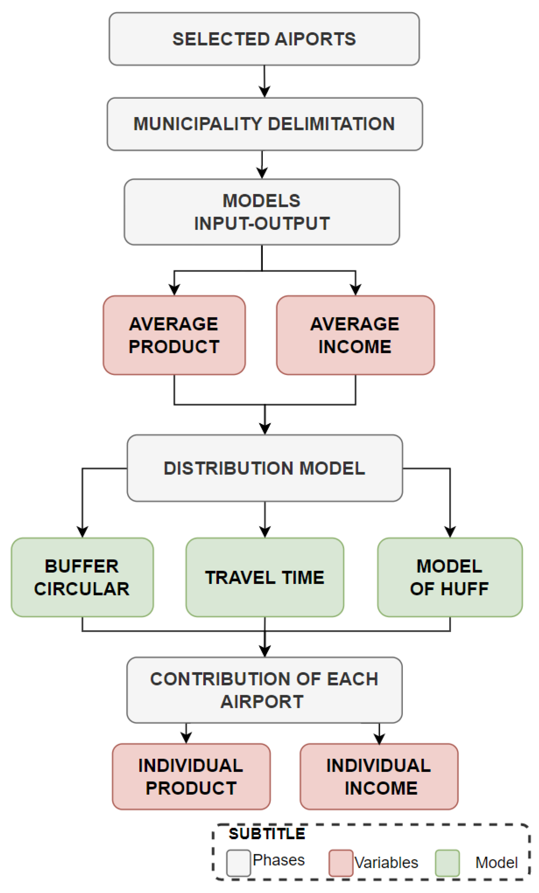
The data analysis was conducted in the following order: first, the airports were selected and the municipalities within a 200 km radius were identified. Next, the IO tables were analyzed to obtain economic data for these cities. The IO analysis determined two average multipliers: generated product and generated income. After obtaining the average multipliers, three distribution models were applied: the circular buffer model, travel time model, and Huff’s model. Finally, the individual contribution of each airport was determined based on the results obtained from applying the distribution models.

Figure 1 presents the flowchart that defines the steps developed in this work. The grey rectangles offer the methodological work stages, the green ones the models adopted in the research, and the red ones the names of the variables that result from the work.

It should be noted that in the analysis of weight models for the input–output method, municipalities located within a 200 km radius of the airport will be considered. Thus, the analysis will be based on the same number of municipalities for all three models. However, each city will have a different weight depending on the methodology adopted by each model.

3.1. Input–Output Method

The IO tables method consists of three matrices: the matrix of intersectoral flows (S-table), the matrix of technical coefficients (A-table), and the matrix of intersectoral impacts (L-table) or the Leontief matrix.

The S-table considers the entire economy disaggregated into N sectors, represented in an NxN arrangement of a square matrix referring to the sectors, plus other inputs (inputs, imports, taxes, and profit margins) and other outputs (exports, government, and final consumers). The sums of the rows and columns for each sector represent, respectively, the total demand and production in a given period. The vectors for total demand and production are equal, indicating the equilibrium state of the economy (LEONTIEF, 1986).

The L-table is obtained by Equation (1). This matrix contains multipliers for calculating the indirect effects (L) of each sector in the economic system.

$$L={(I-A)}^{-1}$$

(1)

where I is the identity matrix and the matrix L is the inverse of the difference between the identity matrix I and table A. It is called the L-table or Leontief matrix, simplifying the linear system notation according to Equation (1):

$$X=L\times Y$$

(2)

The Y vector consolidates the exogenous demand (consumption) data to the sectors that build the A-table to calculate the vector X of production needed to meet such a demand.

The L-table has the same dimensions as the A-table and positive numerical coefficients, eventually greater than 1, called economic impact multipliers, given their algebraic form in determining the effects of demand variation on supply. This relationship is the basis for several analyses and conclusions from the input–output matrices, particularly direct and indirect impact measures.

Impact multipliers are powerful analytical tools associated with input–output matrices. They are dimensionless coefficients that represent the effects in response to any change imposed on an economic system in equilibrium. A measure of an economic sector’s “quality” or “strategic” nature is also used to describe its ability to multiply effects on the economy. Sectors with high multipliers are considered the most relevant because they can trigger more effects on a given expenditure in the face of an incentive.

By definition, a multiplier is calculated based on the hypothesis of adding one unit to the demand of a given sector, assuming that external needs for the rest of the economy remain unchanged. In this sense, for the results of this study, it is considered that the initial effect generated by the increase in one more unit in the demand of a given sector (j) will cause the need for one more unit of products in this sector. In this logic, the “direct impact” is evident, as one more unit of demand will produce one more unit of product, that is, x_j = 1.

It should be considered that the total effect propagates because of the interdependence between sector j and the other sectors of the economy. The greater this interdependence, the more significant the total impact. Thus, it can be seen that if sector j is hypothetically wholly isolated from the rest of the economy, the total effect will be equal to the initial impact. For this reason, the full product includes the initial development, that is, it is the sum of the direct impact with the indirect impacts, where (Equation (3)):

$$\Delta x=L\times f$$

(3)

Therefore, ∆x is the “total effect”, meaning the change in production in all sectors of the economy due to the initial effect in a given sector j. In short, the total impact captures the spread of the initial development to the rest of the economy.

Finally, it is worth mentioning that the estimates of the multipliers calculated by the Leontief matrix in this study follow the economy modeled by the input–output matrix, thus assuming general equilibrium properties [2,7].

The application of IO tables requires official databases on the country’s economy. Therefore, it was essential to extract these data to assess the economics of the air transport sector in the area of influence of airports. Thus, to obtain the input–output matrices, the following banks were consulted:

• IO Tables System for the National Economy: The Center for Regional and Urban Economics of the University of São Paulo (NEREUS) annually publishes good approximations of the IBGE matrices [24], which in turn publishes them every five years. These matrices are calculated according to the recommendations of the Brazilian System of National Accounts;
• IO Tables System for the Region of Study: In the Brazilian case, the primary source of information for constructing the location quotient vector is the data referring to the work factor [16]. The federal government provides detailed microdata on employment and wages, described individually by workers and indexed by the sector of economic activity and municipality. Following the methodology described by [25], it was possible to generate the location quotient vector for the S-table of the 68 industries and obtain the regionalized IO tables. The total remuneration of the labor factor provides good quality regional specialization indexes that are better than if they were obtained only by the number of jobs, especially in a country with solid regional inequalities, such as Brazil [25].

One of the primary challenges encountered in this research pertains to the timeliness of input–output matrices, which serve as crucial data sources for the analysis. As of the publication of this research, the most recently published official Brazilian input–output matrix dates back to 2015. These matrices are typically updated by the NEREUS platform with a lag of five years, resulting in the latest available data being from 2018. This delay severely limits the ability to present current information regarding the Brazilian economy. It is important to note that this delay is not unique to the Brazilian context but is a common issue encountered globally with economic matrices.

3.2. Distribution Models for the Input–Output

The input–output method can be utilized to analyze regions with multiple airports by employing a weighted analysis of the attractiveness of each airport, as discussed by Wang et al. [26]. In such cases, the Leontief matrix’s weights can be determined by either deterministic or probabilistic models proposed by Huber and Rinner [10]. Deterministic models are used when the airports in the study area have similar attractiveness and are based on physical parameters such as distance radius and displacement time to the airport. Two examples of deterministic models are the circular buffer and displacement time models. On the other hand, probabilistic models consider factors such as airport attractiveness, travel time, and the number of flights. One example of a probabilistic model is the Huff model, which can be used to determine airport weights in the Leontief matrix.

In this study, we will apply the circular buffer, displacement time, and Huff models to determine the weights of the Leontief matrix for the airports in our region of interest. By considering various factors that impact the attractiveness of each airport, these models will help provide a more accurate analysis of the economic impact of the air transport sector.

3.3. Circular Buffer Model

The most common economic sharing analysis method is establishing a circle centered on the reference point [27]. This model allows an initial approximation of the radius of influence of each point of interest. However, circular buffers can be inaccurate in areas with natural faults, such as rivers, lakes, and mountains, or poor road connectivity [10]. In such cases, the area inside the circle may be inaccessible to users. Furthermore, it may slightly skew the results because, in this case, all cities within the operating radius will have a defined weight regarding the model’s center. This weight can be expressed by Equation (10):

$$P_{ik}^{BC}=1-\frac{D_{ik}^{}}{{\displaystyle \sum _{j=1}^n{D}_{jk}^{}}}$$

(4)

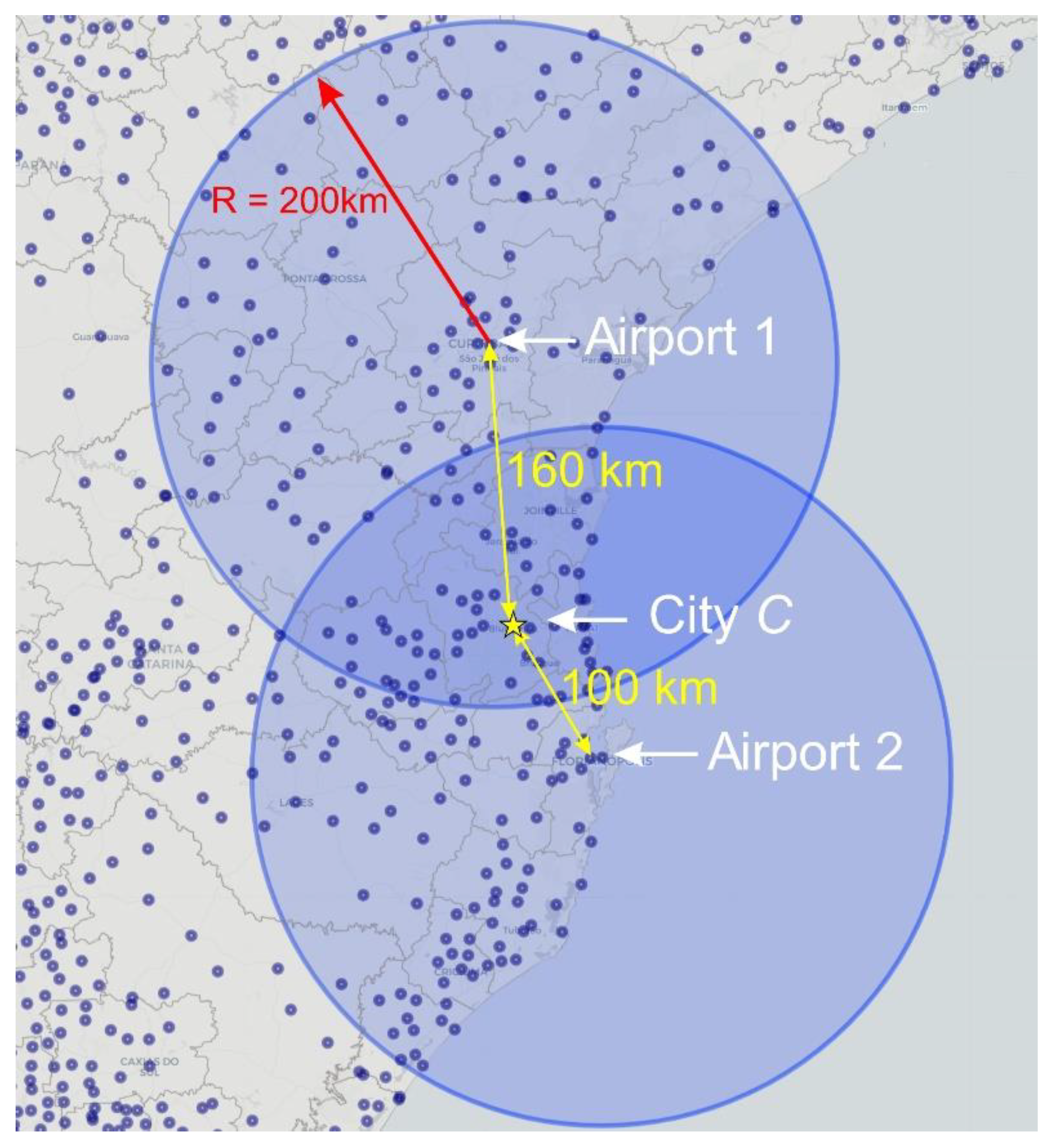
where P^BC is the weight of the circular buffer model relative to the straight-line distance from airport i to city k, n is the number of airports impacting the city’s economy, and D is the distance to the airport. For better definition, the circular buffer model will analyze two airports in which the operating radius is estimated to be 200 km. In this case, the savings from air transport will be split between both airports.

Thus, the economic benefits of air transport for cities within the circular buffer zones will be allocated based on the Euclidean distance from the airports. Therefore, airports closer to the city will have a higher weight in the air transport sector’s impact on these cities’ economies.

For a better illustration, Figure 2 presents the circular buffer model for two airports, estimating the radius of operation to be 200 km. In this case, the economic benefits resulting from air transportation will be divided between these two airports.

The relative influence of airport 1 on city C will be given by:

$$P_{1C}^{BC}=1-\frac{160}{160+100}\approx 0.385=38.5\%$$

(5)

The relative influence of airport 2 on city C will be given by:

$$P_{2C}^{BC}=1-\frac{100}{160+100}\approx 0.615=61.5\%$$

(6)

It can be noted that this model is conservative, given that:

$$P_{1C}^{BC}+P_{2C}^{BC}=100\%$$

(7)

Thus, the economy of air transportation in cities located at the intersections of circular buffers will be distributed based on the straight-line distance from the airports. Airports that are closer to the city will have a greater impact on the economy of air transportation in those cities.

3.4. Travel Time Model

Due to the limitation of circular buffers, some studies use travel time to define the economic share of the region [10]. This model represents reality better, as it can predict natural limiting conditions such as the site’s topography. This analysis can be performed by calculating the distance to a given reference point through Google Maps.

Instead of using circular buffers, which have some limitations, some studies utilize travel time to determine the economic share of a region [10]. This model provides a more realistic representation of reality since it can account for natural limiting conditions, such as the area’s topography. The travel time analysis can be conducted by calculating the distance to a specific reference point using tools such as Google Maps [28].

The formulation of the time–distance model is quite similar to the circular buffer model. However, the model employs the minimum travel time between the city and the airport instead of a straight-line distance. Thus, it can be written as Equation (8):

$$P_{ik}^{TD}=1-\frac{T_{ik}^{}}{{\displaystyle \sum _{j=1}^n{T}_{jk}^{}}}$$

(8)

where P^TD represents the weight assigned to the travel time models. The variable n denotes the number of airports that have an impact the city’s economy, whereas T represents the minimum displacement time from a user located at the center of downtown city k to the airport i.

For a better illustration, Figure 3 presents the travel time from a user located in city C for two random airports.

The relative influence of airport 1 on city C will be given by:

$$P_{1C}^{TD}=1-\frac{245}{245+138}\approx 0.713=36.03\%$$

(9)

The relative influence of airport 2 on city C will be given by:

$$P_{2C}^{TD}=1-\frac{138}{245+138}\approx 0.286=63.97\%$$

(10)

3.5. Huff’s Gravitational Model

When multiple airports serve a common region, each of them can be considered to have a certain level of attractiveness to that region’s public. Therefore, academics and analysts extensively use the probabilistic model of spatial consumer behavior introduced by Huff in 1964 in various applications, including air transport [29,30]. Generally, the results obtained using Huff’s probabilistic model are more realistic than those obtained using deterministic models, as the former considers the variability in the attractiveness of each airport [10]. The model is based on the principle that the probability of a given consumer visiting and using a given location is a function of the distance from that location, its attractiveness, and the distance and attractiveness of other competing sites.

The popularity of Huff’s model can be attributed to its conceptual appeal, ease of handling, and applicability to a wide range of problems [29]. It is applied when one wants to understand the spatial behavior of a given population. The probability that a consumer located at point i will choose to go to an attractive point j is represented by P_ij in this model Equation (11):

$$P_{ij}=\frac{A_j^{\alpha }{D}_{ij}^{-\beta }}{{\displaystyle \sum _{j=1}^n{A}_j^{\alpha }{D}_{ij}^{-\beta }}}$$

(11)

where Aj is the measure of the attractiveness of j, D_ij is the distance from i to j, α is the parameter of beauty estimated from empirical observations, β is the decay parameter of the distance calculated from empirical observations, and n is the total number of attractive points j.

The quotient of division $A_j^{\alpha }$ by $D_{ij}^{-\beta }$ is the attractiveness that point j arouses in the consumer at i. The parameter α is an exponent that considers the nonlinear behavior of the attractiveness variable. The parameter β models the decay rate in the attraction potential of point i as consumers move away from j. Increasing this exponent will increase the relative influence of a point of attraction j on more distant consumers.

For a better illustration, consider that in Figure 2, airport 1 handled 6.5 million passengers and airport 2 handled 3.8 million passengers over a year. In this case, the economic benefits resulting from air transportation will be divided between these two airports as in the following relationship:

$$P_{1C}=\frac{6.5\times {160}^{-1}}{3.8\times {100}^{-1}+6.5\times {160}^{-1}}\approx 0.517=51.7\%$$

(12)

$$P_{2C}=\frac{3.8\times {100}^{-1}}{3.8\times {100}^{-1}+6.5\times {160}^{-1}}\approx 0.483=48.3\%$$

(13)

As it may be inferred, in Huff’s model, the attractiveness coefficient tends to increase the proportionality of airport 1 in the study.

4. Results and Discussion

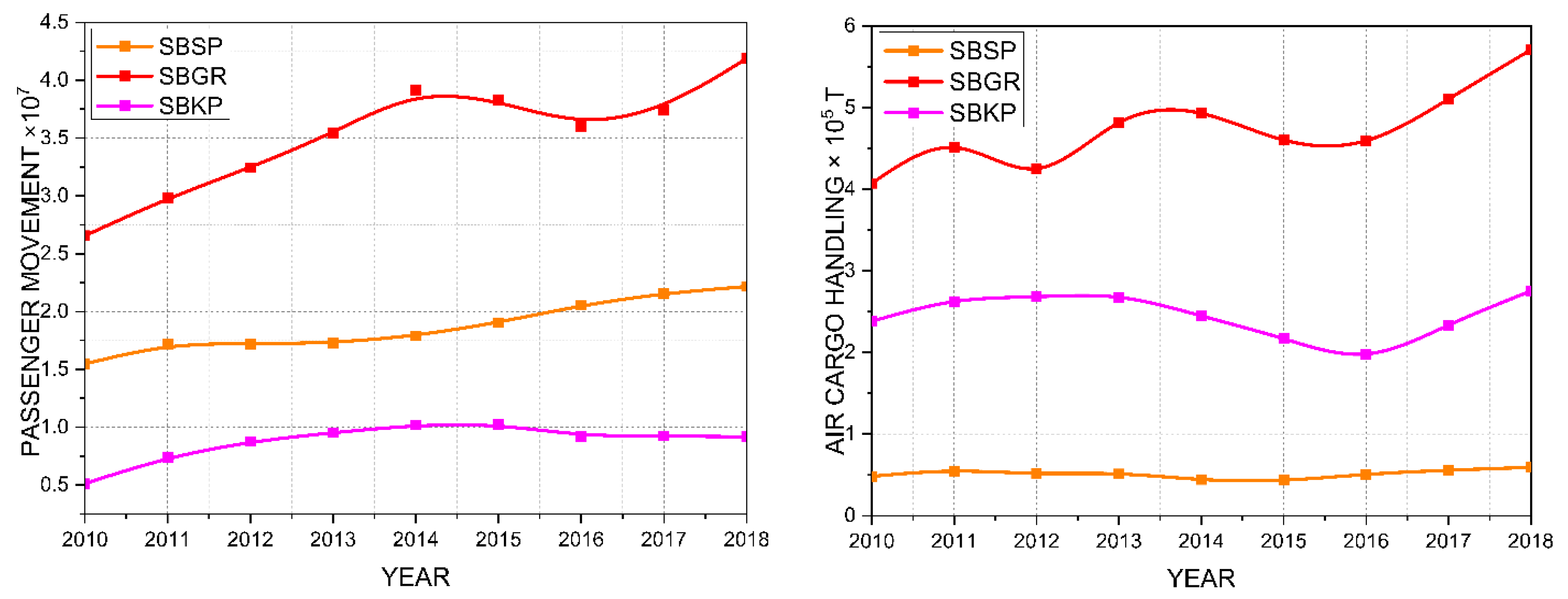
São Paulo is home to three airports that stand out regarding passenger and air cargo movement. As one of the critical states in Brazil, São Paulo’s economy relies heavily on the industrial, transportation, and tourism sectors. Figure 4 shows the total passenger movement, which includes both international and domestic passengers, at Viracopos International Airport (SBKP), Governador André Franco Montoro Airport (SBGR), and Deputado Freitas Nobre Airport (SBSP), which collectively represent a significant portion of the country’s air transport. SBKP and SBGR were conceded to the private sector in 2012, whereas SBSP Airport was conceded in 2011.

It is worth noting that passenger movement grew at all three airports. However, it is also important to mention some shocks to the evolution of the economy. During this period, two major economic shocks occurred that significantly impacted the air transport sector. The first was the FIFA World Cup 2014^TM, which resulted in substantial investments in the transport and infrastructure sectors. Moreover, Brazil attracted a large number of tourists in 2014 to attend the event, leading to a surge in air transport passenger movements. The second significant event was the Brazilian economic crisis, which ultimately led to the president’s impeachment process in 2016. This crisis had a profound impact on various industries, including air transport.

SBGR saw an increase of approximately 56% between 2010 and 2018, although there was a reduction in passenger movement between 2014 and 2016 before resuming growth in 2017. The crisis impacted passenger movement at this airport, reducing it by 9.8% between 2014 and 2016. Passenger movement at SBSP increased by about 47% between 2010 and 2018, stabilizing between 2011 and 2014 before growth continued in 2015. When analyzing SBKP, there was an almost 90% increase in passenger movement between 2010 and 2018. The development started in 2010 and continued to a peak in 2014, after which there was a slight decrease in the movement of passengers in the terminal.

Figure 4 also displays the annual tonnage of air cargo movement at SBSP, SBGR, and SBKP. From 2010 to 2018, the cargo handling capacity at the main terminal in the country grew by 67.5%. However, there were significant oscillations during the growth period, with 2012, 2015, and 2016 standing out for this airport. The Brazilian crisis between 2014 and 2016 affected air cargo movement at SBGR and SBKP, reducing it by approximately 10%. SBSP restricts the size of aircraft it can accommodate. Thus, operations with enormous aircraft are not feasible. Due to these restrictions, air cargo movement is restricted and remained constant throughout the period.

On the other hand, SBKP serves as an alternative terminal to SBGR for cargo transport in São Paulo. The data reveals that this airport experienced modest growth of about 10% between 2010 and 2018. However, it is noteworthy that the cargo handling at SBKP peaked in 2012 and 2013, followed by a decline to the lowest point in 2016.

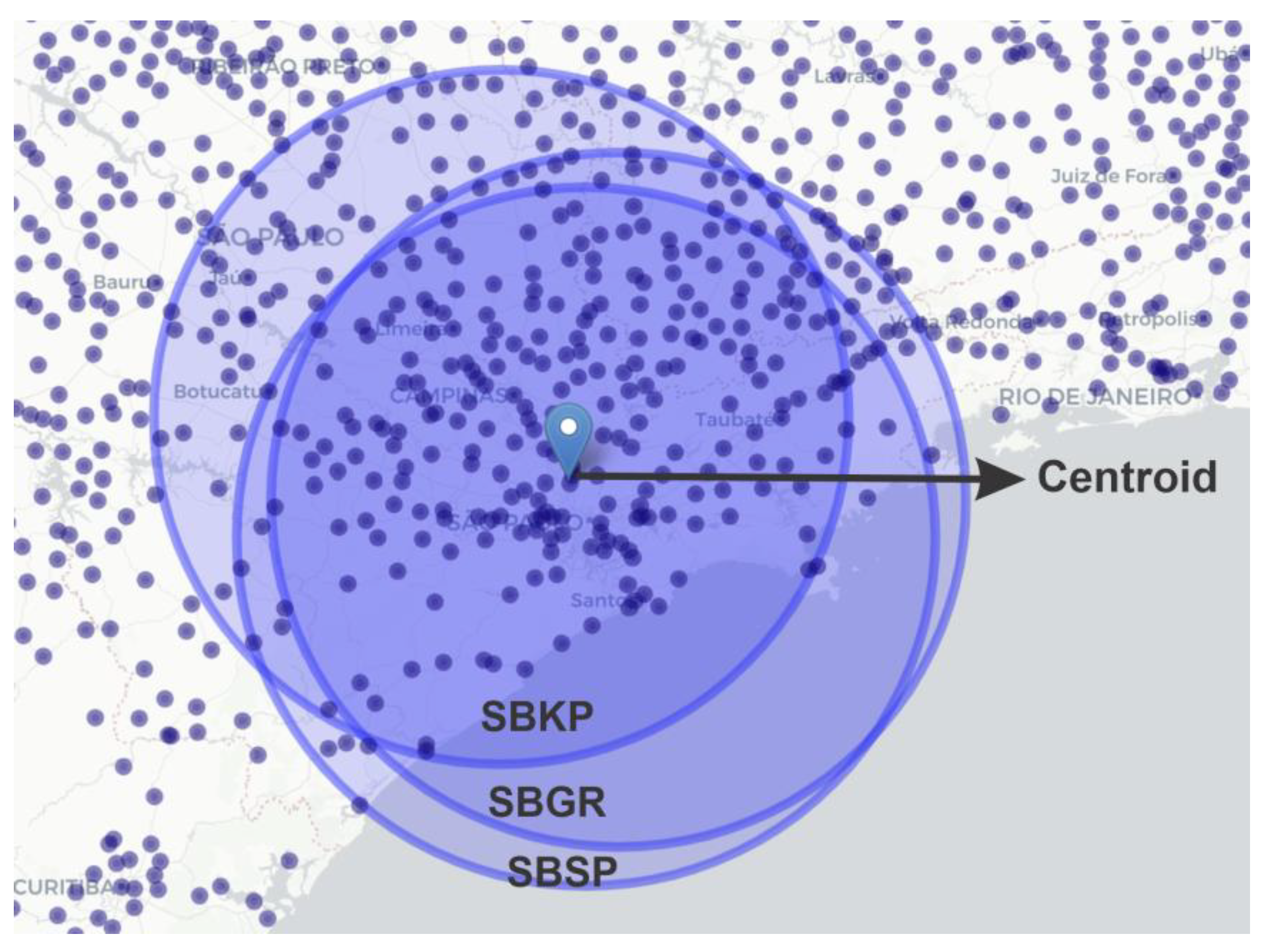
Figure 5 displays the catchment area of the three airports analyzed in São Paulo. SBKP, located further inland, has a catchment area that differs slightly from that of SBSP and SBGR. As a result, SBKP can serve users from more inland regions of São Paulo and southern Minas Gerais. Although the three airports share a large catchment area, further investigation is necessary to determine the individual contributions of each airport to the regional scenario.

4.1. Study of Attractiveness Coefficients for the Region of São Paulo

Table 2. Attractiveness coefficient according to the travel time model for SBSP, SBKP, and SBGR.

Airport	SBSP	SBKP	SBGR
T(P, A)	0.264	0.424	0.312

displays the probability of a user located in one of the cities within the catchment areas of the airports presented in Figure 2 selecting an airport based on the travel time required to reach them. Again, it is evident that, in terms of travel time, SBKP has a higher probability of being selected than SBSP or SBGR, albeit with a slight advantage for the latter.

Table 3. Attractiveness coefficient according to the circular buffer model for SBSP, SBKP, and SBGR.

Airport	SBSP	SBKP	SBGR
D(P, A)	0.237	0.521	0.242

presents the probability that a user that is in one of the cities in the areas of influence of the airports shown in Figure 6 chooses one of the options, considering only the travel time taken from his position to the airport. It is observed that, based on this aspect, SBKP has a greater probability of being chosen than the SBSP or SBGR, in which case both airports would have practically the same probability of choice.

This section examines the Huff coefficients based on the time a user travels from a municipality P to an airport k. The classic Huff study used the straight-line distance from a user to a store [29]. However, this method does not consider geographic barriers, such as uneven terrain, which can affect travel time. Thus, the displacement time model for data analysis was adopted in this study.

Table 4. Attractiveness coefficient according to the Huff model for SBSP, SBKP, and SBGR.

Year	SBSP	SBKP	SBGR
2010	0.287	0.266	0.446
2011	0.276	0.292	0.431
2012	0.265	0.304	0.431
2013	0.257	0.307	0.436
2014	0.252	0.306	0.442
2015	0.259	0.306	0.435
2016	0.274	0.296	0.43
2017	0.277	0.291	0.432
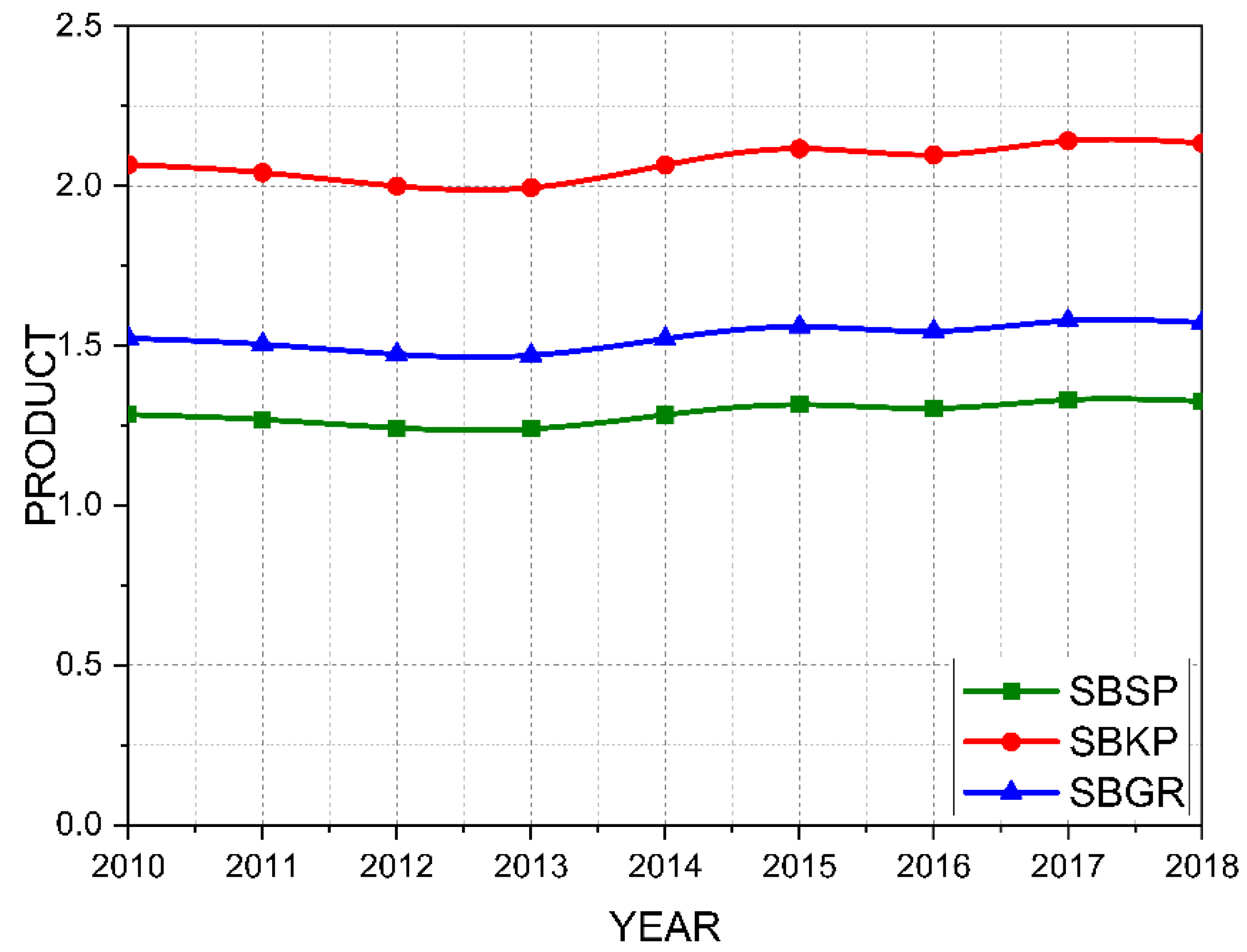
2018	0.273	0.282	0.445

presents the attractiveness coefficient according to the Huff model for the airports SBSP, SBKP, and SBGR. The Huff model considers airport attractiveness parameters that can vary periodically. Therefore, an annual evaluation was chosen for the coefficient associated with the Huff model. During the analyzed period, it was observed that SBGR showed stability in terms of regional relevance. On the other hand, SBSP had a slight drop in regional significance, followed by an increase of similar magnitude for SBKP.

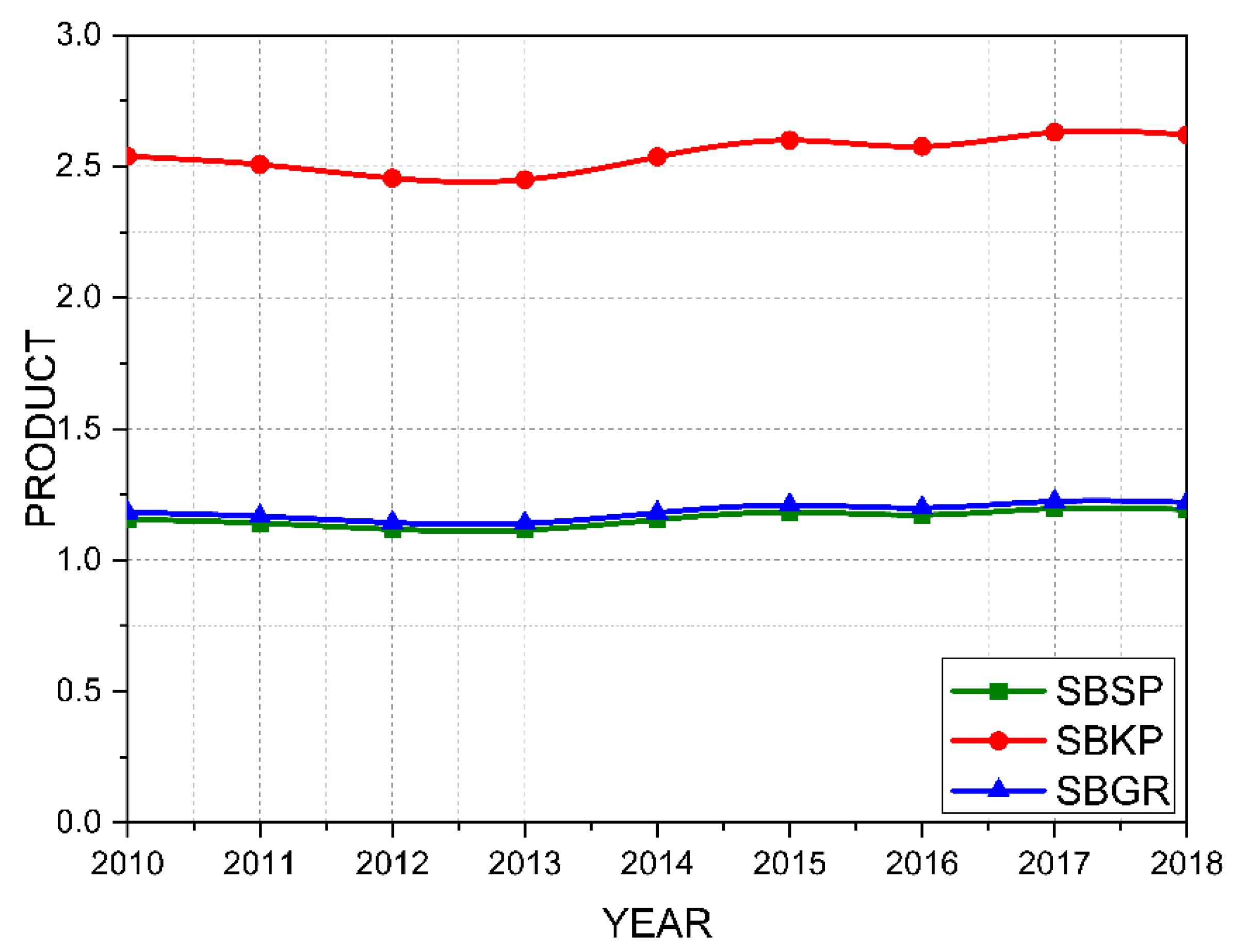
Figure 6 presents the results for the variable product for the three analyzed airports using the circular buffer model. Based on the data presented in Figure 4, SBGR is expected to have a higher product generation since it concentrates on a greater air cargo volume. However, analyzing SBKP using the circular buffer model in Figure 6, it is observed that the theoretical values for the product variable expected for this terminal are higher than those of the buffer model for SBGR or SBSP. Through this analysis, it can be concluded that for every monetary unit invested in SBKP, 2.5 monetary units are generated, whereas for SBGR or SBSP, each economic unit invested generates 1.2 monetary units. This occurs because the circular buffer model considers that the user’s choice is based on the straight-line distance to the airport. Thus, the airport closest to a higher number of users receives a greater weight in the division of economic data. Based on this model, it can be concluded that SBKP has a better geographic and strategic position than SBGR or SBSP. Therefore, the geographic location tends to favor product generation in Campinas.

In this case, the buffer model can show that there is a greater propensity for product generation when investments are made in SBKP. However, the buffer model does not consider the location’s geography or ground transportation means. For example, there may be a natural barrier that the user must circumvent. In this case, the travel time model may be a better indicator for predictive analysis.

The travel time model considers that the user chooses an airport based on the time it takes to travel from one airport to another. Therefore, the weights associated with each airport in this model consider that users choose airports closer to their starting point. In addition, unlike the circular buffer model, the travel time model considers the existing ground infrastructure for airport access.

Figure 7 presents the results for the product variable for the three analyzed airports using the weight distribution of the travel time model. In this case, it is observed that SBKP has a higher attractiveness for more users. This is because the average travel time from the analyzed cities to SBKP is equivalent. Therefore, through this model, it can be perceived that SBKP has better accessibility than SBGR or SBSP. Thus, being closer to more users, SBKP presents a higher product valuation than SBGR or SBSP. This may indicate that if investments are directed towards SBKP, more users will likely choose to use this airport than SBGR or SBSP. However, this analysis tends to be flawed in one aspect. When the region has airports with different attractions, users may choose a more distant airport because only the more distant airport can provide the service they need. Thus, distribution based solely on travel time may not be realistic. In this case, it is necessary to include factors related to the attractiveness of each airport.

Therefore, the most realistic analysis should consider factors that will lead a user to choose one airport over another. In this case, probabilistic models are more suitable for analysis than statistical models. In this case, research by the Huff model can be used to determine the actual values associated with the product generated by each airport. This is because the Huff analysis considers factors of the attractiveness of the three airports. Thus, it can confirm what is expected in the study of this section: SBGR should present a higher product generation because it concentrates the most significant movement of passengers and air cargo in the country.

As can be inferred, the circular buffer and travel time models lack sensitivity to the economic shocks that occurred during the period. In these models, the distribution tends to remain stable regardless of the shocks. However, by using an improved model, it becomes possible to capture the changes that occur and how they affect the distribution of the product variable.

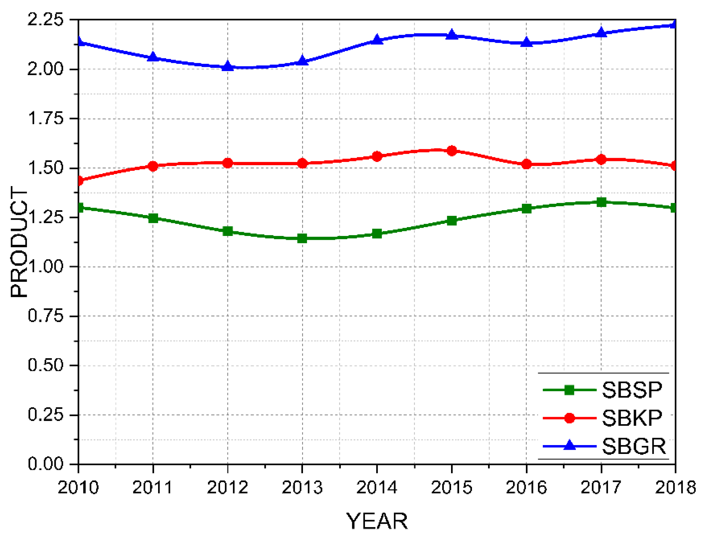
Figure 8 presents the multiplier of the product variable for the three airports analyzed using the weighting factor of the Huff model. In this case, when passenger and air cargo movement are considered attractive factors, SBGR presents higher product generation than SBKP and SBSP. This analysis shows the expected division of GDP generation in the region considering data such as the transportation movement of people and goods. Adapting the Huff model proposed in this work considers factors such as the user’s travel time to the airport and attractiveness parameters such as the movement of passengers and air cargo. Due to these considerations, the Huff model can be expected to present a more realistic approach to calculating the weights associated with air transportation. From the analysis of Figure 8, it is possible to notice that for each monetary unit invested in SBGR in 2018, there was a return in the product of 2.25 monetary units. By the analysis by Huff model, the second most influential airport in the region is SBKP, which generates a multiplier of 1.5× for each real investment. Finally, São Paulo Airport generates an associated product of 1.3× compared with the investment made.

Table 5. Average updated product for São Paulo airports.

Airport	Average	Standard Deviation	Margin of Error (~95% I.C.)
SBSP	1.2435	0.067	0.0438
SBKP	1.5241	0.027	0.027
SBGR	2.1218	0.0466	0.0466

presents the updated average product for the airports in the state of Sao Paulo. It can be observed that SBGR has an average multiplier for the period of 2.1218. This means that for every monetary unit invested in SBGR, a return of 2.1218× is expected. Among the three analyzed airports, it can be observed that SBGR has the highest return, followed by SBKP and lastly, the least profitable is SBSP. Based on the analysis of the product variable, the Huff model indicates that investing in SBGR would be more suitable. However, using the travel time model, the most suitable airport for investment is SBKP, as it is located in a better strategic geographic position than SBSP or SBGR and has the potential to serve more users.

4.2. Income Variable

The variable “income” is a multiplier considering the direct and indirect effects of income associated with the air transportation sector. The value associated with the income multiplier means that for each monetary unit invested in the air transportation sector, there is a return of x in terms of salaries. In this case, larger airports with many employees allocate a significant portion of their investment to maintain operations and pay their staff. The three models showed significant differences when analyzing the results proposed for the income variable.

Although the evaluated income remains stable in general, there is a notable change in 2015 due to the economic crisis in Brazil. This crisis resulted in a significant number of job losses, particularly among lower-level workers. Consequently, the average salary increased, leading to a divergence in the income trend observed in the models.

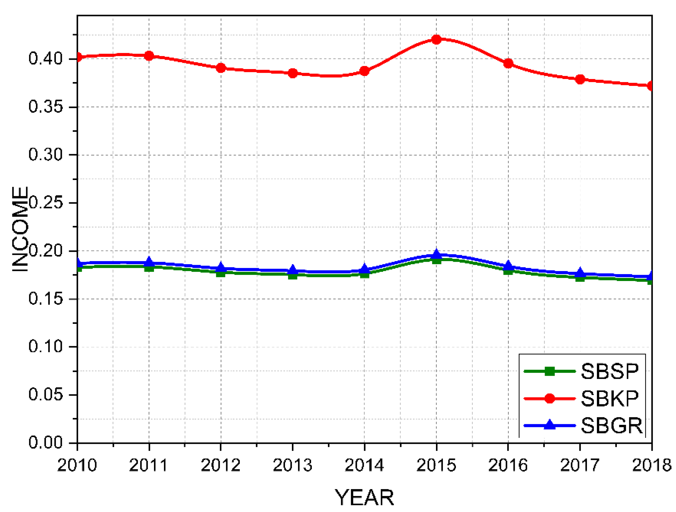
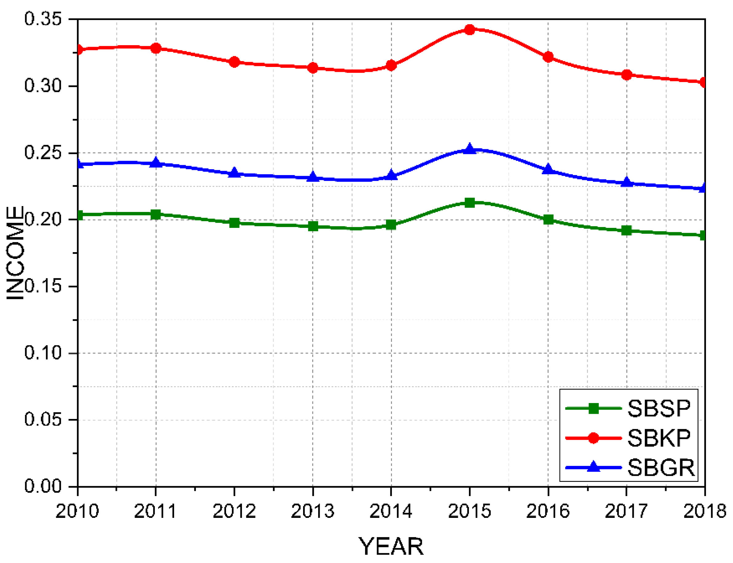
Figure 9 shows the income variable for the three analyzed airports using the circular buffer distribution model. Again, SBKP showed a higher return than SBSP and SBGR. Based on the analysis in Figure 9, SBKP is expected to have a return of about 0.37× the investment made as direct income associated with air transportation. On the other hand, SBSP and SBGR have a return of about 0.17× the investment made as immediate income. However, the distribution of this data does not align with expectations, as one would expect SBSP to have a higher return as it relies on a larger number of employees to maintain its operation.

Figure 10 shows the income variable for the three analyzed airports using the travel time model. If the three airports were able to offer the same service and the user could choose between any of them based solely on travel time, the income return for the airports would be as shown in Figure 10. In this case, the income variable for SBKP in 2018 was 0.3, whereas it was 0.23 for SBGR and 0.18 for SBSP.

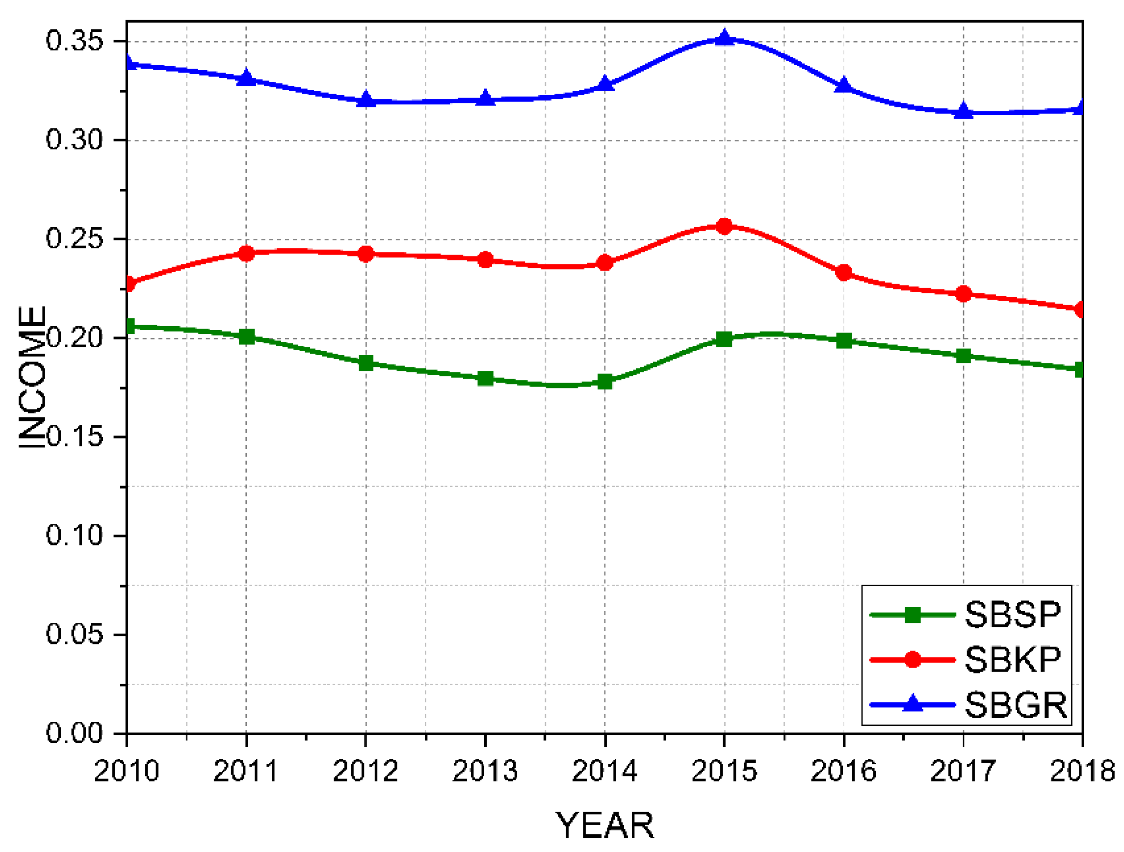
Taking attractiveness into account provides a more realistic understanding of each airports’ contributions to the income associated with air transport in the period shown. Figure 11 shows the income variable for the three airports analyzed using the Huff model. In this case, the Huff model yields a result closer to the expected outcome. It can be observed that SBGR has a more significant impact on the income associated with air transport in the region than SBKP or SBSP.

Table 6. Updated average income for São Paulo airports.

Airport	Average	Standard Deviation	Margin of Error (~95% I.C.)
SBSP	0.1918	0.0100	0.3273
SBKP	0.2353	0.0123	0.0117
SBGR	0.3273	0.0082	0.0077

presents the updated average income for the airports in São Paulo. The data obtained from the Huff model were taken into consideration. It can be observed that SBGR has an average multiplier for the period of 0.3273. This means that for every monetary unit invested in SBGR, an expected return of 0.3273× is generated as the payment of salaries and consequent income generation. Among the three airports analyzed, it is observed that SBGR has the highest return, followed by SBKP, and finally, the airport that would spend the least on salaries is SBSP.

Based on the analysis of the income variable, there is a higher probability that investments made in SBGR will be converted into salaries, as indicated by the Huff model. This happens because SBGR already has an extensive infrastructure and the investment required for payments is high. Thus, a significant portion of the investment is intended for salary payments. On the other hand, if we consider the travel time model, the airport that would generate more income would be SBKP, which does not reflect reality since SBKP’s operation is smaller than SBGR’s. Therefore, the Huff model is considered more suitable for distribution.

5. Conclusions

This study proposes a methodology that combines the IO tables model and distribution models for economic analysis of a region based on the presence of airport infrastructure. The proposed method is an alternative for analyzing a region with two or more airports. The study provides a distribution of economic data associated with three airports in the state of São Paulo: Guarulhos International Airport—Governor André Franco Montoro (SBGR), Viracopos International Airport (SBKP), and Congonhas International Airport Deputado Freitas Nobre (SBSP).

The study considers air traffic and economic data from 2010 to 2018 and brings an innovative method to obtain the significant economic impacts at airports that compete for the same influence area. Unlike other studies that analyze only one airport or locations close to it, this study presents three important characteristics: (i) the use of IO tables to regionalize the municipalities of the influence area of the airport facilities under study, (ii) the economic effect results for some of the airports with the highest passenger and air cargo movements in the country, and (iii) the use of three different models of weights to determine the attractiveness coefficient of each airport. The deterministic models analyzed are the buffer and travel time, and the probabilistic model is the Huff model, which is associated with the airport’s attractiveness. In addition, the modeling adopted a geographic and temporal approach to quantify the impact of airports in regions with an overlap of influence.

The study of the attractiveness coefficient through the Huff model shows that SBGR represents about 44.5% of the users’ preference in São Paulo. Additionally, the annual analysis shows that SBGR has a consolidated position compared with its peers from 2010 to 2018.

However, the attractiveness coefficients according to both the travel time and circular buffer models show that SBKP has a strategic geographical position. In this case, SBKP has the ability to be more accessible to the vast majority of users from SBGR and SBSP. Therefore, if investments are made to expand and popularize SBKP, the geographical location should favor product generation in the state. As a result, when analyzing the generation of product and income, SBGR has the highest generation of product and income in the analyzed region, followed by SBKP and then SBSP.

The analysis carried out proved to be important for identifying trends in the attractiveness of regional sectors. The three models prove to be useful for analysis. However, the circular buffer and travel time models do not take into account the effects of economic shocks on the distribution. They assume a constant distribution pattern, regardless of external factors. By improving the model, it becomes possible to capture the changes that occur and how they affect the distribution of the variables. The Huff model presents the current scenario based on the attractiveness of each airport. These values make it possible to determine the contribution of each airport to the regional scenario and assist in determining user consumption trends. The travel time model presents an idealistic view, where the user’s decision is based solely on travel time. This model is useful in cases where a company wants to offer a service to a specific region. Thus, it would be possible to compare the airport in which an investment would be made with its peers to identify which market share the airport can gain considering the existing ground infrastructure. Finally, the circular buffer model idealizes the travel time model case. In this case, the time the user would take to reach the airport is ignored. Instead, the user’s decision is based on the straight-line distance. This model is useful in analyzing where investors can improve not only airport infrastructure but also access to the airport. Therefore, it can be concluded that each model is useful in a particular case and it is difficult to determine the best model among the three.

Thus, this study aims to develop tools for investors and public managers in decision making and investment allocation related to airport infrastructure. The developed models are expected to be applied to determine investment opportunities or better use of public resources. One of the main limitations of this study is the uncertainty associated with the estimation of the attractiveness coefficients, particularly the λ parameter of the Huff model, which is an empirical parameter reflecting the effect of distance between an airport and a municipality. Additionally, the attractiveness of an airport was assumed to be solely a function of passenger and air cargo movements, which may not accurately reflect the true attractiveness of an airport. Therefore, it is suggested to collect empirical data to evaluate the attractiveness of airports and determine which services impact consumer preference when choosing an airport. This could be achieved by conducting a survey at airports in the State of São Paulo to determine user preferences and the attractiveness associated with each airport.

Another suggestion would be to expand the analysis nationally and re-evaluate the country’s main cargo and passenger airports. This expansion would allow for data collection on the national airport scenario, determining the most attractive terminals and their main contributions to Brazil’s GDP. By doing so, it would be possible to identify key investment and resource allocation areas for public managers and investors in the airport industry.