Analysis of the Performance of Machine Learning Models in Predicting the Severity Level of Large-Truck Crashes

Abstract

Large-truck crashes often result in substantial economic and social costs. Accurate prediction of the severity level of a reported truck crash can help rescue teams and emergency medical services take the right actions and provide proper medical care, thereby reducing its economic and social costs. This study aims to investigate the modeling issues in using machine learning methods for predicting the severity level of large-truck crashes. To this end, six representative machine learning (ML) methods, including four classification tree-based ML models, specifically the Extreme Gradient Boosting tree (XGBoost), the Adaptive Boosting tree (AdaBoost), Random Forest (RF), and the Gradient Boost Decision Tree (GBDT), and two non-tree-based ML models, specifically Support Vector Machines (SVM) and k-Nearest Neighbors (k-NN), were selected for predicting the severity level of large-truck crashes. The accuracy levels of these six methods were compared and the effects of data-balancing techniques in model prediction performance were also tested using three different resampling techniques: Undersampling, oversampling, and mix sampling. The results indicated that better prediction performances were obtained using the dataset with a similar distribution to the original sample population instead of using the datasets with a balanced sample population. Regarding the prediction performance, the tree-based ML models outperform the non-tree-based ML models and the GBDT model performed best among all of the six models.

1. Introduction

In the United States, large trucks, as a significant means of freight transportation, play a major role in the transportation system. Crashes associated with large trucks often lead to substantial economic costs and serious or even fatal injuries. Accurate prediction of the severity level of a reported truck crash can help rescue teams and emergency medical services take the right actions and provide proper medical care, thereby reducing its economic and social costs.

In general, the following KABCO scale is frequently used by law enforcement for classifying the severity levels of a crash: K stands for fatal injury, A stands for incapacitating injury, B stands for non-incapacitating injury, C stands for possible injury, and O stands for no injury. In crash severity prediction studies, the response classes are often categorized into different levels, including two levels, three levels, and so on [1]. The response classes are usually determined by the research objectives and data quality. Detailed information about crash datasets will be presented in the data collection and description section.

A variety of modeling methods have been used in previous studies to predict crash severity. These methods include both traditional regression models and Machine Learning (ML)-based methods. Traditional regression methods are not good at capturing and interpreting associations between independent variables and dependent variables due to the limitation of predefined assumptions [2]. Therefore, recently, many researchers have turned to ML methods, and various ML methods have been adopted for crash prediction purposes. Among them, the Decision Tree, Support Vector Machine (SVM), and k-Nearest Neighbor (k-NN) methods have been widely employed for crash severity prediction. It is unclear, however, whether different types of ML-based models perform equally well. In addition, to develop a reliable prediction model, some attention has been paid to the selection of sample datasets for training classifiers. Some researchers concluded that a training sample with a skewed class distribution tends to make classifiers biased [3]. To solve this issue, some researchers suggest using a dataset with a balanced number of instances of different classes, while other scholars suggest that it is more beneficial to use a sample that has a class distribution the same as its population [4]. Indeed, in crash severity prediction, the number of instances relating to AK-level crashes is generally far fewer than the number of instances relating to non-AK-level crashes. Therefore, the effects of different data-balancing methods on the prediction performance of different modeling approaches need to be investigated.

This study aims to investigate the performance of different ML methods in predicting the severity levels of large-truck crashes and the effects of data-balancing techniques on model prediction performance. First, three resampling techniques, namely random undersampling, SMOTE oversampling, and mix sampling, were used to pre-process the original training dataset. Then, six representative machine learning methods, including four classification tree-based ML models, specifically the Extreme Gradient Boosting tree (XGBoost), Adaptive Boosting tree (AdaBoost), Random Forest (RF), and Gradient Boost tree (GBDT), and two non-tree-based ML models, specifically Support Vector Machines (SVM) and k-Nearest Neighbors (k-NN), were selected to predict the severity level of large-truck crashes. After that, the performances of different models using different types of training datasets were compared and analyzed.

In this study, an overview of previous research on the subject was summarized and then the dataset used for his study was explained, and the analysis methodology was introduced. Finally, a thorough discussion of the modeling outcomes and their implications was discussed, and further suggestions were made.

2. Literature Review

2.1. Crash Severity Prediction Models

Previous studies have investigated different aspects of traffic safety analysis: Single-vehicle crashes and multi-vehicle crashes, pedestrian collisions, macro-level crash analysis, and micro-level crash analysis. For example, Wei et al. (2021) proposed a novel Bayesian spatial random parameters logit (SRP-logit) model to explore the risk factors associated with the severity of rural single-vehicle (SV) crashes [5]. The results indicated that the SRP-logit model exhibits the best-fit performance compared with the multinomial logit model, random parameter logit model, and random intercept logit model.

Guo et al. (2018) compared different approaches to modeling macro-level cyclist safety. Four types of models were developed: The Poisson lognormal model (PLN), random intercepts PLN model (RIPLN), random parameters PLN model (RPPLN), and spatial PLN model (SPLN) [6]. The SPLN model performed best, and the results highlighted the significant effects of spatial correlation.

Cai et al. (2021) investigated the factors associated with the severity of low-visibility-related rural single-vehicle crashes [7]. In their study, a latent class clustering model was implemented to partition the whole dataset into sub-datasets before modeling. Then, a spatial random parameters logit model was established for each dataset to capture unobserved heterogeneity and spatial correlation.

Among all the modeling approaches, ML techniques stand out as an alternative to statistical methods. A variety of ML modeling methods have been adopted in all aspects of crash-safety studies, including decision tree models, neural networks, Support Vector Machines, and ensemble learning classifiers. In particular, there is growing interest in using tree-based ML techniques to predict and identify crash severity.

Li et al. (2012) compared the performance of the Support Vector Machine (SVM) model and the ordered probit (OP) model in predicting the injury severity associated with individual crashes [8]. It was found that the SVM model produced a better prediction performance for crash injury severity than the OP model.

Pineda-Jaramillo et al. (2022) used a set of machine-learning models to predict the severity of a vehicle–pedestrian collision. The results showed that the Linear Discriminant Analysis model surpasses other machine learning models considering the evaluation metrics [9].

Chang and Chien (2013) examined the effects of factors related to drivers and vehicles on heavy-truck crashes using the classification and regression tree method [10].

Yu and Abdel-Aty (2014) developed a crash severity analysis regression model by first identifying factors that can explain the occurrence of severe crashes through a random forest approach [11].

Iranitalab and Khattak (2017) compared the performance of Multinomial Logit, Nearest Neighbor Classification, Support Vector Machines, and Random Forests in crash risk prediction. In their study, the effects of data clustering preprocessing were also investigated [12]. Although the results indicated that clustering methods can improve prediction performance under certain conditions, in the real world, it is not practical to cluster a crash before its crash severity can be predicted.

Tang et al. (2019) proposed a two-layer crash severity predicting framework [13]. The first layer incorporates three tree-based models: Random Forest, an Adaptive Boosting tree, and a Gradient Boost Decision tree. The second layer combines all the prediction results of the developed tree-based models through logistic regression.

Schlögl et al. (2019) conducted a comparison of seven methods for identifying contributing factors to traffic crashes [14]. A series of statistical learning techniques (including all four types of logistic regression, tree-based ensemble methods, the BRNN, and the Pegasos SVM) were compared regarding their predictive performance. The results showed good performance of tree-based methods.

2.2. Data Balancing Techniques in Crash Severity Prediction Modeling

To develop a reliable prediction model, some attention has been paid to the selection of appropriate sample datasets for training or fitting models. As we know, high-imbalance datasets often occur in real-world applications. Trained with such a dataset, standard ML classifiers tend to be biased [3]. The effects of class imbalance have attracted more and more attention in recent years. To solve this issue, previous studies have proposed solutions from the dataset perspectives and algorithmic perspectives. From the dataset perspective, one can use many different forms of resampling to preprocess the data to obtain balanced training datasets. At the algorithmic level, solutions include creating new algorithms or modifying existing ones. Compared with the algorithmic level approach, the data-level approach seems to be more straightforward and has greater promise to overcome the class-imbalance problem [15]. Therefore, this study focuses on the data preprocessing perspective. In general, three types of resampling approaches can be used to balance classes. These are oversampling methods, undersampling methods, and mixed methods. Oversampling includes the techniques that balance the number of instances between classes by increasing the number of minority classes until the distribution of classes is balanced, while undersampling includes the techniques to balance classes by reducing the number of instances from the majority class. Finally, mixed techniques include techniques that integrate the above two techniques.

In recent years, several studies have explored crash severity prediction with data-balancing techniques. For example, Mujalli et al. (2016) discussed the effects of three types of different data-balancing approaches on traffic crash data [16]. Then, Bayes classifiers were developed based on the imbalanced and balanced datasets. It was found that using the balanced training datasets reduced the misclassification of AK-level crashes.

Schlögl et al. (2019) adopted a mixed approach in which a combination of oversampling and undersampling was used to preprocess the dataset [14]. The findings revealed that there is a trade-off between accuracy and sensitivity. They conclude that this was inherent to imbalanced classification problems.

Rivera et al. (2020) assessed five classification algorithms on an original imbalanced dataset [17]. Five re-sampling algorithms were tested: The synthetic minority oversampling method (SMOTE), borderline SMOTE, adaptive synthetic sampling, random undersampling, and random oversampling. The results indicated that the imbalance between binary labels negatively affected the performance of both classifiers. Moreover, random oversampling performs best.

Abou Elassad et al. (2020) developed a decision support system based on four ML methods [18]. This study also studied the effects of three balancing methods: Oversampling, undersampling, and synthetic minority over-sampling (SMOTE). The best performances were acquired by SMOTE balancing.

In summary, various ML-based modeling approaches have been used to predict crash severity. Among these models, classification tree-based ML models (e.g., Extreme Gradient Boosting tree (XGBoost), Adaptive Boosting tree (AdaBoost), Random Forest (RF), and Gradient Boost Decision Tree (GBDT)), Support Vector Machines (SVM), and k-Nearest Neighbors (kNN) are the most popular ML techniques that have been used for crash severity prediction. However, it is unclear whether different types of ML-based models perform equally well. Moreover, few studies have considered the tree-based ML models as a group and compared them with other types of ML methods. Several questions remain open and need further exploration. Therefore, this study aims to compare the performances of six machine learning models in predicting large-truck crash risk. In addition, the effects of the data imbalance issue on the performance of different modeling approaches are still not clear. To fill this gap, the three most commonly used data balancing techniques, random undersampling, SMOTE oversampling, and mix sampling, will be used to preprocess the original training dataset to test the effectiveness of data balancing in model prediction performance.

3. Study Data

3.1. Data Source

The truck crash records of the state of Texas from 2016 to 2019 were pulled from the Texas Crash Records Information System (CRIS). In the raw dataset, there are over 170 attributes in each record, including information about the drivers, the number of vehicles involved, crash characteristics, weather conditions, and roadway location and conditions.

3.2. Variables Selection and Setting

The severity level of crashes was the prediction label. It was categorized into three levels: Crashes with Property Damage Only (PDO) (y = 0), crashes with Slight Injuries (SLIG) (y = 1), and crashes in which someone is Killed or has Severe Injuries (KSEV) (y = 2). In the training dataset, as shown in Figure 1a, there were 72.45% PDO-level crashes, 22.84% SLIG-level crashes, and 4.71% KSEV-level crashes. In the testing dataset, as shown in Figure 1b, there were 73.36% PDO-level crashes, 22.27% SLIG-level crashes, and 4.37% KSEV-level crashes. It can be seen that the data are very imbalanced because a class distribution with an imbalance ratio greater than 1.5 can be considered imbalanced [19], and the distribution of the three severity levels of the testing dataset is highly consistent with that of the training dataset.

Forty independent variables were carefully selected from over 170 attributes based on the analysis of their correlations and data quality. These attributes of the large-truck crash data belong to different categories, as shown in

Table 1. Variables and Descriptions.

Traffic Control		Weather Characteristics
none	1 for no traffic control, 0 otherwise (baseline)	clr	1 for clear weather condition, 0 otherwise (baseline)
st_sign	1 for traffic control is stop sign, 0 otherwise	rain	1 for raining weather condition, 0 otherwise
sig_light	1 for signal light controlled, 0 otherwise	snw	1 for snowing weather condition, 0 otherwise
yld_sign	1 for yield sign controlled, 0 otherwise	blowing	1 for blowing sand weather condition, 0 otherwise
flash_light	1 for flashing light controlled, 0 otherwise	fog	1 for fog weather condition, 0 otherwise
mk_lane	1 for markedlane controlled, 0 otherwise	sleet	1 for sleet weather condition, 0 otherwise
sig_camera	1 for signal camera controlled, 0 otherwise	sv_crosswinds	1 for severe crosswinds weather condition, 0 otherwise
Light characteristics		Median type
day_light	1 for crash during daylight, 0 otherwise (baseline)	median_none	1 lane with no median, 0 otherwise (baseline)
dawn	1 for crash during dark yet not lighted, 0 otherwise	unprotected	1 lane with unprotected, 0 otherwise
dk_no_light	1 for crash during dawn, 0 otherwise	posi_barrier	1 lane with positive barrier, 0 otherwise
dk_light	1 for crash during dark yet lighted, 0 otherwise	one_way_pair	1 lane with one-way pair, 0 otherwise
dusk	1 for crash during dusk, 0 otherwise	curbed	1 lane with curbed, 0 otherwise
Roadway functional system		Road alignment
r_int_hwy	1 crashes in rural interstate highway, 0 otherwise (baseline)	stgt_evel	1 for straight level road alignment, 0 otherwise (baseline)
u_int_hwy	1 crash in urban interstate highway, 0 otherwise	stgt_grade	1 for straight grade road alignment, 0 otherwise
r_ppl_a	1 crash in rural principle arterial, 0 otherwise	stgt_hillcrest	1 for straight hillcrest road alignment, 0 otherwise
u_oth_ppl_a	1 crash in urban other principle arterial, 0 otherwise	curve_level	1 for curve level road alignment, 0 otherwise
u_minor_a	1 crash in urban minor arterial, 0 otherwise	curve_grade	1 for curve grade road alignment, 0 otherwise
r_minor_a	1 crash in rural minor arterial, 0 otherwise	curve_hillcrest	1 for curve hillcrest road alignment, 0 otherwise
Location of first harmful event		Base type
on_rd	1 for crash occurred on road, 0 otherwise (baseline)	soil	1 for soil road, 0 otherwise (baseline)
on_shlder	1 for crash occurred on shoulder, 0 otherwise	granular	1 for granular road, 0 otherwise
on_median	1 for crash occurred on median, 0 otherwise	asph	1 for asphalt road, 0 otherwise
off_rd	1 for crash occurred off road, 0 otherwise	concr	1 for concrete road, 0 otherwise
Shoulder type left		Curb type left
shldr_lt_none	1 for no left shoulder, 0 otherwise (baseline)	curb_lt_none	1 for no left curb, 0 otherwise (baseline)
shldr_lt	1 if left shoulder exists, 0 otherwise	curb_lt	1 if left curb exists, 0 otherwise
Shoulder type right		Curb type right
shldr_rt_none	1 for no right shoulder, 0 otherwise (baseline)	curb_rt_none	1 for no right curb, 0 otherwise (baseline)
shldr_rt	1 if right shoulder exists, 0 otherwise	curb_rt	1 if right curb exists, 0 otherwise
Road type		Crash contributing factors
2lane_ 2way	1 for road type that is 2 lanes, 2 way, 0 otherwise (baseline)	fatigue	1 for driver under influence of fatigue, 0 otherwise
4ormore_div	1 for road type that is 4 or more, divided, 0 otherwise	drug	1 for driver under influence of drug, 0 otherwise
4ormore_undiv	1 for road type that is 4 or more, undivided, 0 otherwise	alcohol	1 for driver under influence of alcohol, 0 otherwise
Lane width and shoulder width		Numerical variables
lane_wid	width of lanes in feet	adt_adj_curnt_amt	adjusted average daily traffic for the current year for crashes located on the road
shldr_width_left	width of left shoulder in feet	crash_spd_lim	speed limit of the lane
shldr_width_right	width of right shoulder in feet	trk_aadt_pct	adjusted average daily traffic percent
		nbr_of_lane	number of lanes

. The variable selection process was detailed as follows. The first step is to reduce collinearity variables. Then, categorical variables were converted to dummy variables. It can be observed that the variables in the same category were highly correlated. Taking the “Traffic Control” category as an example, there are six types of traffic control types: “none”, “stopsign”, “signallight”, “yieldsign”, “flashinglight” and “markedlane”, and “signal camera”; in other words, a crash can fall into one of these six conditions. If all these dummy variables were included in modeling, their sum would be equal to 1. This can cause a dummy variable trap, therefore one baseline variable for each category will be selected [20]. Moreover, variables without a clear causal relationship with the dependent variable were removed to avoid the endogeneity problem [21]. Finally, 40 independent variables were selected, as listed in Table 1, and the distributions of variables are presented in

Table 2. Distribution of the Variables.

Variable	Crash Injury Severity			Total	Percent	Variable	Crash Injury Severity			Total	Percent
	PDO	SLIG	KSEV				PDO	SLIG	KSEV
Traffic Control						Weather Characteristics
none	6587	1819	275	8681	10.44%	clr	43,087	13,219	2764	59,070	71.04%
st_sign	2679	915	273	3867	4.65%	rain	6333	1978	332	8643	10.39%
sig_light	7271	2081	253	9605	11.55%	snw	133	26	5	164	0.20%
yld_sign	938	262	28	1228	1.48%	blowing	36	13	8	57	0.07%
flash_light	283	96	32	411	0.49%	fog	422	188	90	700	0.84%
mk_lane	31,653	10,224	1872	43,749	52.62%	sleet	153	35	9	197	0.24%
sig_camera	116	33	5	154	0.19%	sv_crosswinds	159	40	11	210	0.25%
Light Characteristics						Median Type
day_light	45,662	13,980	2326	61,968	74.53%	median_none	17,147	5482	1639	24,268	29.19%
dawn	828	276	84	1188	1.43%	unprotected	5882	1818	368	8068	9.70%
dk_no_light	6667	2249	894	9810	11.80%	posi_barrier	11,128	3634	720	15,482	18.62%
dk_light	6534	2150	480	9164	11.02%	one_way_pair	103	18	1	122	0.15%
dusk	448	139	39	626	0.75%	curbed	675	220	27	922	1.11%
Roadway Functional System						Road Alignment
r_int_hwy	21,967	6639	829	29,435	35.40%	stgt_evel	46,507	14,148	2729	63,384	76.23%
u_int_hwy	5766	1958	733	8457	10.17%	stgt_grade	6265	2161	516	8942	10.75%
r_ppl_a	17,158	5611	769	23,538	28.31%	stgt_hillcrest	1799	741	150	2690	3.24%
u_oth_ppl_a	2348	680	139	3167	3.81%	curve_level	3304	999	265	4568	5.49%
u_minor_a	2853	963	438	4254	5.12%	curve_grade	1947	652	152	2751	3.31%
r_minor_a	6567	1769	538	8874	10.67%	curve_hillcrest	449	121	26	596	0.72%
Location of First Harmful Event						Base Type
on_rd	52,128	16,415	3226	71,769	86.31%	soil	372	133	42	547	0.66%
on_shlder	764	190	130	1084	1.30%	granular	34,451	10,964	2561	47,976	57.70%
on_median	1873	641	115	2629	3.16%	asph	788	223	50	1061	1.28%
off_rd	5653	1608	373	7634	9.18%	concr	24,821	7534	1191	33,546	40.34%
Shoulder Type Left						Curb Type Left
shldr_lt_none	4725	1254	586	6565	8.39%	curb_lt_none	3211	1162	197	4570	27.43%
shldr_lt	51,941	16,290	3459	71,690	91.61%	curb_lt	9225	2518	348	12,091	72.57%
Shoulder Type Right						Curb Type Right
shldr_rt_none	5813	1964	755	8532	10.19%	curb_rt_none	3754	1239	234	5227	29.12%
shldr_rt	54,458	17,180	3573	75,211	89.81%	curb_rt	9721	2636	368	12,725	70.88%
Road Type						Crash Contributing Factors
2lane_2way	9890	3310	1185	14,385	17.30%	fatigue	804	386	129	1319	1.59%
4ormore_div	43,114	13,338	2202	58,654	70.54%	drug	100	84	88	272	0.33%
4ormore_undiv	7355	2189	454	9998	12.02%	alcohol	348	235	167	750	0.90%

. There were 83,148 large-truck crashes in the final dataset.

4. Methodology

4.1. Crash Severity Modeling Methods

As mentioned in the literature review, in this study, six representative machine learning methods, including four representative classification tree-based ML models (e.g., XGBoost, AdaBoost, RF, and GBDT, and two non-tree-based ML models (e.g., SVM and kNN) were selected for developing crash severity prediction models.

4.1.1. Random Forest (RF)

RF builds trees from samples that were drawn from the training dataset. It is a combination of Breiman’s bagging idea and Ho’s “random subspace method” [22]. Decisions are made considering all individual trees in the ensemble. It can be achieved by either averaging the probabilistic predictions of the classifiers or letting each classifier vote.

In this study, the input samples for RF are represented as $\mathrm{x}=\left\{\left[{\mathrm{x}}_{\mathrm{i}1},{\mathrm{x}}_{\mathrm{i}2},...,{\mathrm{x}}_{\mathrm{in}} \right],{\mathrm{y}}_{\mathrm{i}}\right\}$ where i = 1, 2, 3…, m and m indicate the number of crash samples, and n is the number of independent variables. The values of the dependent variable y (y = 0.1, or 2) correspond to different levels of crash severity. The python interface to RF, available through the package RandomForestClassifier from scikit-learn, is used.

4.1.2. Adaptive Boosting (AdaBoost)

AdaBoost is a method of making classifications by combining weak learners with a weighted majority vote (or sum). Taking into account the previous weak learners’ errors, it updated the sample accordingly [23]. The basic steps of this algorithm can be explained as follows [24]:

Given a training dataset $\mathrm{D}=\left\{\left({\mathrm{x}}_1,{\mathrm{y}}_1\right),\left({\mathrm{x}}_2,{\mathrm{y}}_2\right),\cdots ,\left({\mathrm{x}}_{\mathrm{N}},{\mathrm{y}}_{\mathrm{N}}\right)\right\}$, a strong classifier $\mathrm{C}\left(\mathrm{x}\right)$ is generated by the following steps:

Initialization of the weight value distribution of the training data,${\mathrm{W}}_1=\left({\mathrm{w}}_{11},\cdots ,{\mathrm{w}}_{1\mathrm{i}},\cdots ,{\mathrm{w}}_{1\mathrm{N}},\right)$, ${\mathrm{w}}_{1\mathrm{i}}=\frac{1}{\mathrm{N}},\mathrm{i}=1,2,\cdots ,\mathrm{N}$, m = 1, 2,⋯, M (m is the times of iteration).

Using the training dataset as the weight distribution ${\mathrm{W}}_{\mathrm{m}}$ to learn, we obtain the basic classification ${\mathrm{C}}_{\mathrm{m}}\left(\mathrm{x}\right)$ according to the Gini indexes of different influencing factors k.

The classification error rate of ${\mathrm{C}}_{\mathrm{m}}\left(\mathrm{x}\right)$ is calculated as follows:

$${\mathrm{e}}_{\mathrm{m}}=\mathrm{P}\left({\mathrm{C}}_{\mathrm{m}}\left(\mathrm{x}\right)\ne {\mathrm{y}}_{\mathrm{i}}\right)={\displaystyle \sum }_{\mathrm{i}=1}^{\mathrm{N}}{\mathrm{w}}_{\mathrm{mi}}\mathrm{I}\left({\mathrm{C}}_{\mathrm{m}}\left(\mathrm{x}\right)\right)\ne {\mathrm{y}}_{\mathrm{i}}$$

We calculate the “amount of say”, ${\mathrm{a}}_{\mathrm{m}}$ of ${\mathrm{C}}_{\mathrm{m}}\left(\mathrm{x}\right)$ according to its classification error ${\mathrm{e}}_{\mathrm{m}}$

$${\mathrm{a}}_{\mathrm{m}}=\frac{1}{2}\log \frac{1-{\mathrm{e}}_{\mathrm{m}}}{{\mathrm{e}}_{\mathrm{m}}}$$

4.1.3. Gradient Boosting Decision Tree (GBDT)

GBDT is one of the boosting algorithms. The motivation is to combine several weak models to produce a powerful ensemble. Similar to other boosting algorithms, GBDT builds the additive model in a greedy way.

We assume that F(x) is an approximation function of the dependent variable y based on a set of independent variables x. F(x) can be expressed as $\mathrm{F}\left(\mathrm{x}\right)={\displaystyle \sum }_{\mathrm{m}=1}^{\mathrm{M}}{\mathsf{\gamma }}_{\mathrm{m}}{\mathrm{h}}_{\mathrm{m}}(\mathrm{x})$, where ${\mathrm{h}}_{\mathrm{m}}\left(\mathrm{x}\right)$ represents the basic functions that are usually called weak learners in the context of boosting. The loss function can be defined as $\mathrm{L}\left(\mathrm{y},\mathrm{F}\left(\mathrm{x}\right)\right)=\log \left(1+{\mathrm{e}}^{-\mathrm{yF}\left(\mathrm{x}\right)}\right)$. Similar to other boosting algorithms, GBDT builds the additive model in a greedy fashion: The initial model is problem-specific, and for the least-squares regression, one usually chooses the mean of the target values. Gradient Boosting attempts to solve this minimization problem numerically via the steepest descent [24].

4.1.4. Extreme Gradient Boosting (XGBoost)

A variant of gradient-boosted regression trees is Extreme Gradient Boosting (XGBoost) [25]. Due to a number of optimizations—simplifying the objective functions but maintaining the optimal computational speed—XGBoost is a very fast and efficient tree-boosting algorithm [26].

The XGBoost method is based on the processes of additive learning. The first learner is fitted based on the input data, then according to the residuals of the first learner, a second learner is then fitted to reduce the residual of the first weak learner. The model’s final prediction is a summary result of each learner. The python interface to XGBoost, available through package XGboost, is used.

4.1.5. Support Vector Machine (SVM)

A Support Vector Machine (SVM) is a supervised linear classifier that constructs hyperplanes to classify labels [27]. We consider a training set represented by ${\left\{\left({\mathrm{x}}_{\mathrm{i}},{\mathrm{y}}_{\mathrm{i}}\right)\right\}}_{\mathrm{i}=1}^{\mathrm{N}}$, where x_i is the n-dimensional dependent variable and yi represents the independent variable, assume y_i = 1 represents the positive group and the independent variable y_i = −1 represents the negative group. SVM maps each input point x_i in the feature space H and finds a decision surface that separates binary points. The python interface to SVM, available through the package SVM from scikit-learn, is used.

4.1.6. k-Nearest Neighbor (k-NN)

As one of the non-parametric classifiers, k-Nearest neighbor (k-NN) is one of the most commonly used methods [28]. In k-NN, crash records are represented by independent variables as a point in the feature space. When classifying one record of severity, the k-NN classifier assign points based on the distance between the point and the points in the training dataset. In this study, the Euclidean distance is used.

In this study, the python interface to k-NN, available through the package Nearest Neighbors from scikit-learn, is used.

4.2. Data-Balancing Techniques

To test the effectiveness of sampling balancing techniques in detecting the severity level of a large-truck crash, three commonly used resampling approaches were selected to balance the training datasets: The synthetic minority oversampling technique (SMOTE), Random undersampling (RUS), and mixed techniques.

• SMOTE: Using k-Nearest Neighbors, this method aims to create synthetic instances for minority classes [29]. Depending upon the amount of over-sampling required, neighbors from the k nearest neighbors are randomly chosen.
• RUS: Aims to balance the class distribution by randomly eliminating the number of instances of the majority class until the dataset is balanced [3]. The major disadvantage of RUS is that it can delete instances that could be important for data analysis.
• The Mixed technique: This method combines both SMOTE and RUS techniques. In this method, the instance number of the minority class is increased while the instance number of the majority class is discarded until the classes are balanced, while the dataset size remains the same as the original dataset size [16].

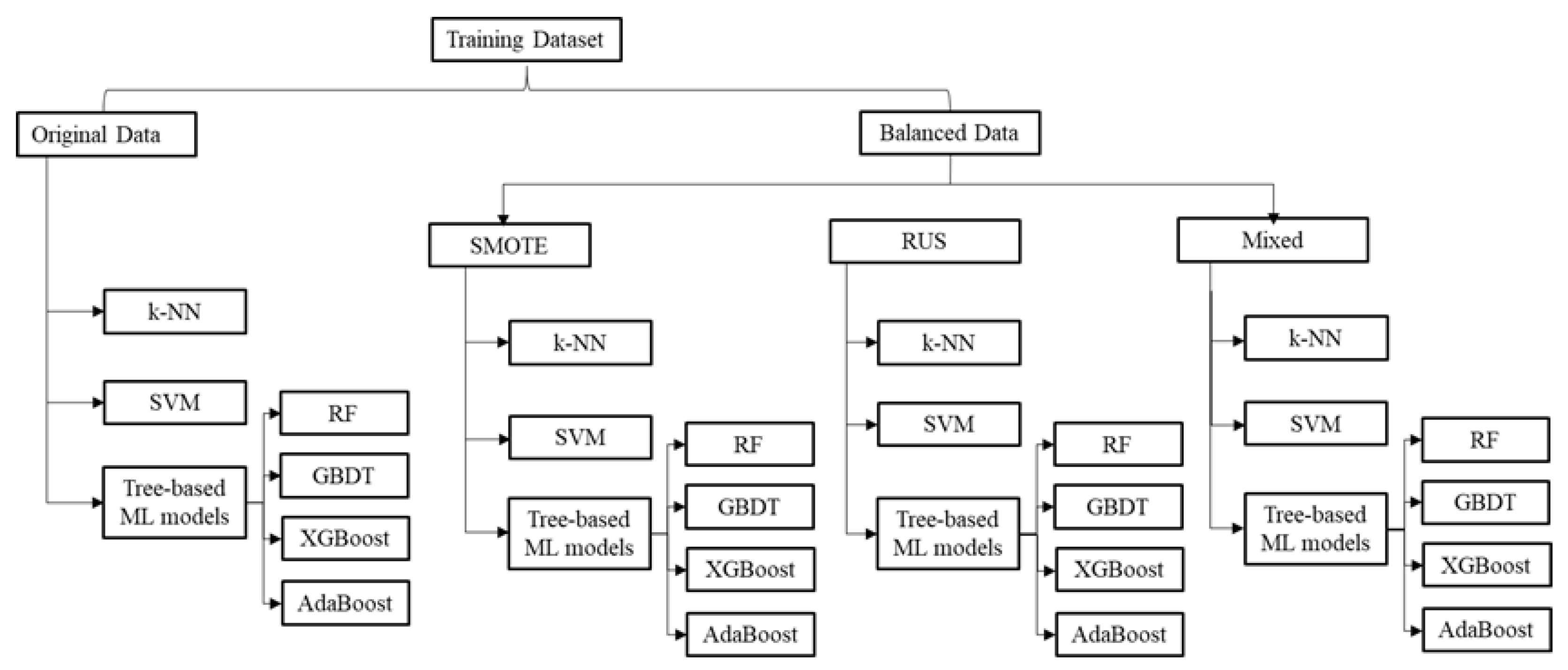
These three resampling techniques are performed in the program python, and the package “imbalanced-learn” is used.

4.3. Study Design

This research was designed to predict the severity level of a large-truck crash based on the comparison of different classification models. As mentioned in the data description section, the final cleaned dataset was divided into a dedicated training dataset (which contains records from the year 2016 to 2018) and a dedicated testing dataset (which contains records from the year 2019). As shown in Figure 2, three resampling techniques including random undersampling, oversampling, and mixed sampling were implemented on the training dataset to create three correspondingly balanced datasets. Together with the original dataset, which is kept the same as the training dataset, a total of four datasets were used to develop different prediction models. Since six classifiers, including four classification tree-based ML models (XGBoost, AdaBoost, RF, and GBDT), and two non-tree-based ML models (SVM and k-NN), were selected in this study, combined with the four datasets, a total of twenty-four prediction models were developed. The effects of class-balancing techniques on model prediction performance were tested by comparing the performance of different models. Figure 2 shows all the modeling scenarios.

4.4. Prediction Evaluation Measures

To evaluate the prediction performance of the model, there were mainly two types of evaluation measures. The first one is threshold-based measures, such as sensitivity, precision, specificity, and the F-measure, which rely on one specific threshold. Since all these measures are decided based on one specific threshold, they cannot provide a comprehensive evaluation of the model performance. This problem can be solved by using non-threshold-based measures, such as ROC-AUC [30].

A Receiver Operator Characteristic (ROC) curve is a graphical plot used to show the diagnostic ability of binary classifiers. A ROC curve is constructed by plotting the true positive rate (TPR) against the false positive rate (FPR) [17], where TPR is the ratio of actual positive instances to all positive instances and FPR is the ratio of actual negative instances to all negative instances [31]. According to this definition, the area under the curve (AUC) indicates the performance of classifiers in separate classes. ROC-AUC values close to 1 describe a highly accurate classifier whereas values close to 0.5 describe a bad classifier [4]. Since there is no specific threshold for ROC-AUC, it can be used to evaluate a prediction model’s overall performance. In addition, ROC-AUC is not biased against the majority class [3]. Therefore, in this study, ROC-AUC is selected as the evaluation measure. In the following parts, ROC-AUC will be simplified as AUC.

5. Results and Analysis

The evaluation has two parts. First, to test the effects of different resampling techniques, the performances of different ML models developed using different training datasets were compared. After that, by using the training dataset that can provide the best performance, the results of different prediction models are further compared and analyzed.

5.1. Imbalanced versus Balanced Training Datasets

This section aims to investigate the effects of sample-balancing techniques on the model’s prediction ability. The original training dataset contained 61,983 crashes in which the severity distribution was 44,905 PDO crashes, 14,159 SLIG crashes, and 2919 KSEV crashes. Three new balanced datasets were created: RUS, SMOTE, and Mixed.

Table 3. Number of Instances in Original and Balanced Training Datasets.

Datasets		Total	PDO	SLIG	KSEV
Original dataset		61,983	44,905	14,159	2919
Balanced datasets	SMOTE	134,715	44,905	44,905	44,905
	RUS	8757	2919	2919	2919
	Mixed	61,983	20,661	20,661	20,661

shows the total number of instances across all datasets and their distribution by severity level.

As shown in Table 3, in the RUS dataset, the number of instances in the resulting datasets for all classes was reduced to the size of the minority class (2925 instances for KSEV). In the SMOTE dataset, the number of instances was increased to 44,905 instances for the PDO class. Finally, in the mixed dataset, the total number of instances of the dataset was kept the same at 61,983 crashes, yet the number of instances was evenly distributed among different classes (the number of instances of the major class was reduced to 20,661 and the number of the instances of the minority class was increased to 20,661).

For each training dataset (original, SMOTE, RUS, and Mixed), six different ML-based modeling methods were applied to develop different models. All the parameters for each model were optimized separately through the function GridSearchCV from scikit-learn until the best AUC score was reached. The testing results of models developed from balanced datasets were then compared with those developed from the original dataset. The AUCs of different models developed from different training datasets are derived and summarized in

Table 4. Overview of AUC Using Different Datasets.

Severity Levels	Datasets	Crash Severity Prediction Models
		XGBoost	GBDT	RF	AdaBoost	k-NN	SVM
PDO	Original	0.59	0.60	0.58	0.58	0.53	0.53
	SMOTE	0.57	0.57	0.57	0.55	0.55	0.51
	RUS	0.57	0.58	0.55	0.57	0.51	0.53
	Mixed	0.53	0.53	0.55	0.53	0.52	0.50
SLIG	Original	0.57	0.58	0.56	0.51	0.53	0.54
	SMOTE	0.55	0.55	0.52	0.51	0.52	0.51
	RUS	0.50	0.51	0.51	0.50	0.51	0.52
	Mixed	0.52	052	0.53	0.49	0.50	0.50
KSEV	Original	0.72	0.72	0.70	0.71	0.62	0.51
	SMOTE	0.70	0.69	0.70	0.67	0.61	0.50
	RUS	0.71	0.72	0.70	0.71	0.62	0.51
	Mixed	0.63	0.62	0.67	0.63	0.57	0.55

Bold: best results for each experiment.

. According to the results presented in Table 4, the following findings can be obtained:

For the tree-based ML methods (XGBoost, AdaBoost, RF, and GBDT), the overall results indicate that the original training dataset works better at predicting all three levels of severity when compared to the balanced datasets. This result is consistent with the findings of Liu et al. (2013) [32]. This result reflects a trade-off between specificity and sensitivity. With the original dataset, classifiers tend to perform better at predicting classes with majority instances and produce lower accuracy over classes with minority instances. Once the dataset is balanced, the accuracy of predicting the minority classes may be increased although at the cost of reducing the prediction accuracy of majority classes. Schlögl et al. (2019) substantiated that a trade-off between accuracy and sensitivity was inherent to imbalanced classification problems [14].

For non-tree-based ML methods (k-NN and SVM), the original dataset also works better. Taking the k-NN classifier as an example, the original dataset works better than the balanced datasets in SLIG- and KSEV-level prediction. Only the SMOTE dataset produced a relatively better PDO-level prediction than the original dataset. The overall results indicate that the original dataset works better in predicting most levels of severity when compared to the balanced datasets. Similar results are obtained for the SVM classifier.

According to Oommen et al. (2010), the imbalanced training dataset will not affect the maximum-likelihood logistic regression model performance if the training dataset has a similar distribution as the testing dataset [4]. In this study, as presented in Figure 1, the distribution of large-truck crash injury severity in training and testing datasets is very similar. Since using an imbalanced training dataset did not affect the model performance for all the tested ML-based models, it seems that Oommen’s conclusion is also applicable to ML-based models.

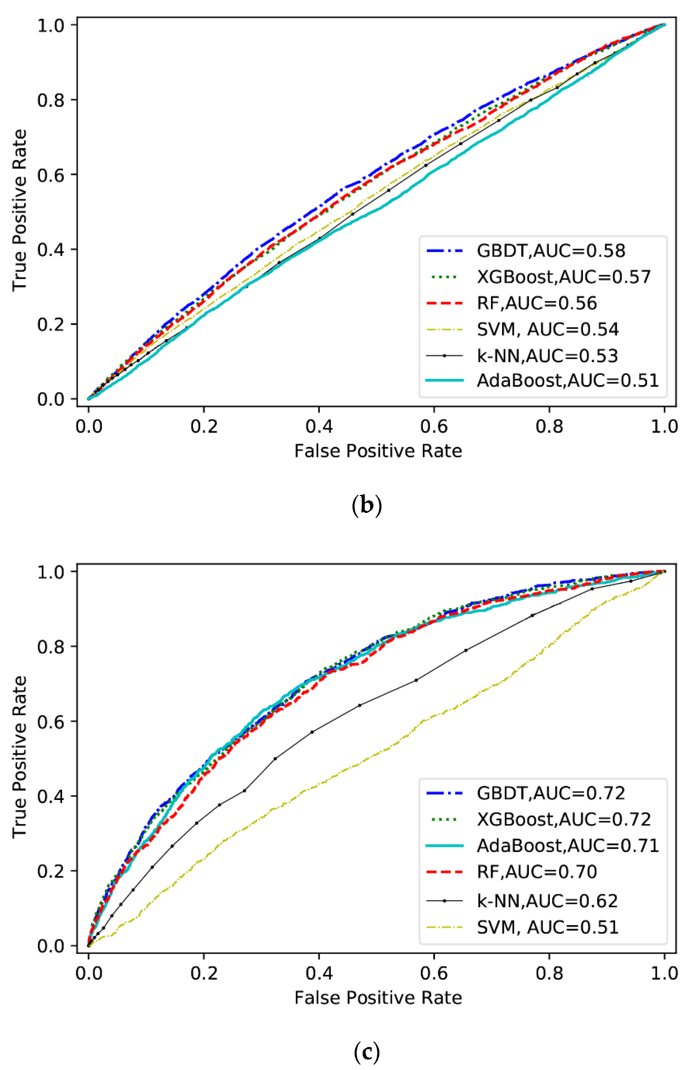
5.2. Prediction Performance of Machine Learning Models

Based on the above results, since there is nearly no improvement achieved by data balancing the training dataset for ML-based models, the original dataset was finally chosen to develop the final prediction models for ML-based models. To make a detailed comparison of the final six models, Figure 3 presents ROC curves of different severity levels.

As shown in Figure 3a, these curves can be divided into two groups, with one group consisting of tree-based models (XGBoost, AdaBoost, RF, and GBDT) and the other group consisting of non-tree-based models (SVM and k-NN). It indicates that the prediction performances of four tree-based ML models are better than the non-tree-based models for predicting PDO-level crashes. The GBDT model showed the best prediction performance.

Similar to Figure 3a, there are two groups of curves in Figure 3b. The difference between these two groups is not as significant as that shown in Figure 3a. One of the tree-based ML methods (AdaBoost) showed relatively low performance, while the other three tree-based algorithms (XGBoost, RF, and GBDT) still performed well. However, GBDT still showed the best results.

As shown in Figure 3c, the four tree-based ML model curves (XGBoost, AdaBoost, RF, and GBDT) are highly overlapped and superior to the other two non-tree-based ML model curves. The two non-tree-based curves are highly separated, and SVM showed the weakest performance.

Overall, all tree-based ML models (XGBoost, AdaBoost, RF, and GBDT) outperform the non-tree-based ML models (SVM and k-NN) at all three severity levels of crash predictions. This result is consistent with Chang and Chien (2013) [10]. They also demonstrated that classification tree analysis is an effective approach for analyzing the injury data of truck crashes. Among the four tree-based models, the GBDT model performs better than the other models.

6. Conclusions and Recommendations

This research was designed to predict the severity level of large-truck crashes based on the comparison of different classification models (XGBoost, AdaBoost, RF, GBDT, SVM, and k-NN). In order to determine the appropriate training dataset for each model, three sampling strategies, namely RUS, SMOTE, and Mixed, were employed to test the effects of data-balancing techniques on the prediction performance of ML-based modeling. The following are the key findings of this study, along with some corresponding recommendations:

• For XGBoost, GBDT, RF, AdaBoost, k-NN, and SVM tested in this study, using an imbalanced training dataset did not affect the model performance. In fact, the original dataset works better in predicting all three levels of severity when compared to the balanced datasets. Therefore, we would recommend using the training dataset that has a similar distribution as the prediction distribution to train the selected ML-based models.
• Classification tree-based ML models (XGBoost, AdaBoost, RF, and GBDT) perform relatively better than the non-tree-based ML models (SVM and k-NN) at all three severity levels. Among them, the GBDT model performs best.

As a result, the results of this study can be used to predict a reported crash whose severity is not known. Moreover, the modeling procedure can provide insight into the selection and development of ML models for large-truck crash severity prediction.

One limitation of the study is that the types of ML models used in this research are limited and the results of resampling may not be applicable to all kinds of ML models. In the future, the authors will further test the effectiveness of resampling in neural network modeling, Naive Bayes modeling, and so on. Furthermore, the modeling approach used in this study can be expanded to analyze other traffic safety problems such as crash frequency for different types of road function systems. In addition, it would also be interesting to explore the results of smaller data-balancing intervals.

References

1. Fiorentini, N.; Losa, M. Handling imbalanced data in road crash severity prediction by machine learning algorithms. Infrastructures 2020, 5, 61. [Google Scholar] [CrossRef]
2. Su, X.; Zhou, T.; Yan, X.; Fan, J.; Yang, S. Interaction trees with censored survival data. Int. J. Biostat. 2008, 4, 1–26. [Google Scholar] [CrossRef] [Green Version]
3. Kotsiantis, S.; Kanellopoulos, D.; Pintelas, P. Handling imbalanced datasets: A review. GESTS Int. Trans. Comput. Sci. Eng. 2006, 30, 25–36. [Google Scholar]
4. Oommen, T.; Baise, L.G.; Vogel, R.M. Sampling bias and class imbalance in maximum-likelihood logistic regression. Math. Geosci. 2011, 43, 99–120. [Google Scholar] [CrossRef]
5. Wei, F.; Cai, Z.; Wang, Z.; Guo, Y.; Li, X.; Wu, X. Investigating Rural Single-Vehicle Crash Severity by Vehicle Types Using Full Bayesian Spatial Random Parameters Logit Model. Appl. Sci. 2021, 11, 7819. [Google Scholar] [CrossRef]
6. Guo, Y.; Osama, A.; Sayed, T. A cross-comparison of different techniques for modeling macro-level cyclist crashes. Accid. Anal. Prev. 2018, 113, 38–46. [Google Scholar] [CrossRef]
7. Cai, Z.; Wei, F.; Wang, Z.; Guo, Y.; Chen, L.; Li, X. Modeling of Low Visibility-Related Rural Single-Vehicle Crashes considering Unobserved Heterogeneity and Spatial Correlation. Sustainability 2021, 13, 7438. [Google Scholar] [CrossRef]
8. Li, Z.; Liu, P.; Wang, W.; Xu, C. Using support vector machine models for crash injury severity analysis. Accid. Anal. Prev. 2012, 45, 478–486. [Google Scholar] [CrossRef]
9. Pineda-Jaramillo, J.; Barrera-Jiménez, H.; Mesa-Arango, R. Unveiling the relevance of traffic enforcement cameras on the severity of vehicle–pedestrian collisions in an urban environment with machine learning models. J. Saf. Res. 2022, 81, 225–238. [Google Scholar] [CrossRef]
10. Chang, L.-Y.; Chien, J.-T. Analysis of driver injury severity in truck-involved accidents using a non-parametric classification tree model. Saf. Sci. 2013, 51, 17–22. [Google Scholar] [CrossRef]
11. Yu, R.; Abdel-Aty, M. Utilizing support vector machine in real-time crash risk evaluation. Accid. Anal. Prev. 2013, 51, 252–259. [Google Scholar] [CrossRef]
12. Iranitalab, A.; Khattak, A. Comparison of four statistical and machine learning methods for crash severity prediction. Accid. Anal. Prev. 2017, 108, 27–36. [Google Scholar] [CrossRef] [PubMed]
13. Tang, J.; Liang, J.; Han, C.; Li, Z.; Huang, H. Crash injury severity analysis using a two-layer Stacking framework. Accid. Anal. Prev. 2019, 122, 226–238. [Google Scholar] [CrossRef] [PubMed]
14. Schlögl, M.; Stütz, R.; Laaha, G.; Melcher, M. A comparison of statistical learning methods for deriving determining factors of accident occurrence from an imbalanced high resolution dataset. Accid. Anal. Prev. 2019, 127, 134–149. [Google Scholar] [CrossRef] [PubMed]
15. Thammasiri, D.; Delen, D.; Meesad, P.; Kasap, N. A critical assessment of imbalanced class distribution problem: The case of predicting freshmen student attrition. Expert Syst. Appl. 2014, 41, 321–330. [Google Scholar] [CrossRef] [Green Version]
16. Mujalli, R.O.; López, G.; Garach, L. Bayes classifiers for imbalanced traffic accidents datasets. Accid. Anal. Prev. 2016, 88, 37–51. [Google Scholar] [CrossRef]
17. Rivera, G.; Florencia, R.; García, V.; Ruiz, A.; Sánchez-Solís, J.P. News classification for identifying traffic incident points in a Spanish-speaking country: A real-world case study of class imbalance learning. Appl. Sci. 2020, 10, 6253. [Google Scholar] [CrossRef]
18. Abou Elassad, Z.E.; Mousannif, H.; Al Moatassime, H. A proactive decision support system for predicting traffic crash events: A critical analysis of imbalanced class distribution. Knowl.-Based Syst. 2020, 205, 106314. [Google Scholar] [CrossRef]
19. Fernández, A.; García, S.; del Jesus, M.J.; Herrera, F. A study of the behaviour of linguistic fuzzy rule based classification systems in the framework of imbalanced data-sets. Fuzzy Sets Syst. 2008, 159, 2378–2398. [Google Scholar] [CrossRef]
20. Greene, W.H. Econometric Analysis, 4th ed.; International Edition; Prentice Hall: Hoboken, NJ, USA, 2000. [Google Scholar]
21. Duncan, G.J.; Magnuson, K.A.; Ludwig, J. The endogeneity problem in developmental studies. Res. Hum. Dev. 2004, 1, 59–80. [Google Scholar]
22. Breiman, L. Random forests. Mach. Learn. 2001, 45, 5–32. [Google Scholar] [CrossRef] [Green Version]
23. Chen, S.-H.; Pan, J.-S.; Lu, K. Driving Behavior Analysis Based on Vehicle OBD Information and Adaboost Algorithms. In Proceedings of the International Multiconference of Engineers and Computer Scientists, Hong Kong, China, 18–20 March 2015; pp. 18–20. [Google Scholar]
24. Li, J.; Liu, J.; Liu, P.; Qi, Y. Analysis of factors contributing to the severity of large truck crashes. Entropy 2020, 22, 1191. [Google Scholar] [CrossRef] [PubMed]
25. Fan, J.; Wang, X.; Wu, L.; Zhou, H.; Zhang, F.; Yu, X.; Lu, X.; Xiang, Y. Comparison of Support Vector Machine and Extreme Gradient Boosting for predicting daily global solar radiation using temperature and precipitation in humid subtropical climates: A case study in China. Energy Convers. Manag. Sci. 2018, 164, 102–111. [Google Scholar] [CrossRef]
26. Chen, T.; Guestrin, C. Xgboost: A Scalable Tree Boosting System. In Proceedings of the 22nd ACM SIGKDD International Conference on Knowledge Discovery and Data Mining, San Fransico, CA, USA, 13–17 August 2016; pp. 785–794. [Google Scholar]
27. Vapnik, V. The Nature of Statistical Learning Theory; Springer Science & Business Media: Berlin, Germany, 1999. [Google Scholar]
28. Cover, T.; Hart, P. Nearest neighbor pattern classification. IEEE Trans. Inf. Theory 1967, 13, 21–27. [Google Scholar] [CrossRef] [Green Version]
29. Chawla, N.V.; Bowyer, K.W.; Hall, L.O.; Kegelmeyer, W.P. SMOTE: Synthetic minority over-sampling technique. J. Artif. Intell. Res. 2002, 16, 321–357. [Google Scholar] [CrossRef]
30. Fernández, A.; García, S.; Galar, M.; Prati, R.C.; Krawczyk, B.; Herrera, F. Learning from Imbalanced Data Sets; Springer: Berlin, Germany, 2018; Volume 10. [Google Scholar]
31. Wei, F.; Cai, Z.; Guo, Y.; Liu, P.; Wang, Z.; Li, Z. Analysis of roadside accident severity on rural and urban roadways. Intell. Autom. Soft Comput. 2021, 28, 753–767. [Google Scholar] [CrossRef]
32. Liu, X.; Zhou, Z. Ensemble methods for class imbalance learning. In Imbalanced Learning: Foundations, Algorithms, and Applications; Wiley: Hoboken, NJ, USA, 2013. [Google Scholar]
Figure 1. Distribution of Large-Truck Crash Injury Severity in Training and Testing datasets. (a) Training dataset. (b) Testing dataset.
Futuretransp 02 00052 g001
Figure 2. Study Scenarios.
Futuretransp 02 00052 g002
Figure 3. Comparison of Prediction Performance of Different Models. (a) ROC curves of PDO-level crash prediction. (b) ROC curves of SLIG-level crash prediction. (c) ROC curves of KSEV-level crash prediction.
Futuretransp 02 00052 g003aFuturetransp 02 00052 g003b