Article

Optimal Transport Pricing in an Age of Fully Autonomous Vehicles: Is It Getting More Complicated?

by
Stefan Tscharaktschiew
1,* and
Christos Evangelinos
2
1
Institute of Transport and Economics, Technische Universität Dresden, 01062 Dresden, Germany
2
Department Aviation Management, IU International University of Applied Sciences, 10247 Berlin, Germany
*
Author to whom correspondence should be addressed.
Future Transp. 2022, 2(2), 347-364; https://doi.org/10.3390/futuretransp2020019
Submission received: 17 January 2022 / Revised: 29 March 2022 / Accepted: 30 March 2022 / Published: 6 April 2022

Abstract

:
Over the last several decades, transportation scientists have made substantial progress in identifying and tackling transport-related problems by elaborating sophisticated policy instruments. Originally, the policy instruments were developed and designed to tackle inefficiencies caused by conventional (human-driven) vehicles. However, questions remain regarding transportation policies, especially pricing instruments, in the future. With the advent of fully autonomous vehicles (driverless or self-driving cars), many of potentially disruptive changes to our transportation system are projected to occur. This gives rise to the question of how to adapt the existing, well established, policy instruments to make them applicable to a world of self-driving cars. The present paper utilizes one of the most widely deployed, most important (in terms of tax revenue), and most effective (in terms of carbon dioxide mitigation) current price-based policy instruments in the transport sector (i.e., the energy tax) to show how one of the most innovative features associated with fully autonomous vehicles (i.e., driverless vehicle relocation) affects the optimal design of a transportation tax. We adopt a microeconomics optimization framework and analytically derive the optimal energy tax under the assumption that driverless vehicle relocation is possible. Our main finding is that in a world of self-driving cars, the energy tax (likewise, a second-best miles tax) as a price-based policy instrument becomes more difficult to evaluate. With the capability of fully autonomous vehicles to relocate without passengers inside, the (analytical) expression for the optimal energy tax becomes more complex, and its (numerical) determination becomes more difficult since the feature of driverless vehicle repositioning imposes counteracting welfare effects as a response to a tax change. Policymakers and researches are encouraged to take on the challenge of increasing complexity to tackle transport-related inefficiencies in the era of self-driving cars.

1. Introduction

Over the last several decades, transportation scientists have made substantial progress in identifying and tackling transport-related problems (see, e.g., [1,2]). In fact, many of the proposals made by researchers have already been put into effect, or have at least contributed to a growing awareness and knowledge of transport-related problems and their long-term consequences. There are numerous examples, especially in regard to price-based measures, which are usually favored by economists: congestion pricing [3,4,5,6,7], energy/fuel taxation [8,9,10,11,12], parking pricing [13,14,15,16,17], and public transport subsidies [18,19,20,21], to name a few. To account for the complications associated with real-world problems, the methods and tools developed and applied by researchers have been continuously developed and improved. Examples include the heterogeneity of travelers, interactions with the broader fiscal system and the rest of the economy, and uncertainty (see [22]).
One area that requires further consideration is transportation policies, especially pricing instruments, in the future. Originally, they were developed and designed to tackle inefficiencies caused by conventional (human-driven) vehicles. With the advent of fully autonomous vehicles (also referred to as driverless or self-driving cars), however, many potentially disruptive changes to our transportation system are projected to occur [23,24,25,26]. The potential changes concern, for example, safety issues in terms of a predicted substantial reduction in road crashes, the way travelers may engage in more productive and more pleasant activities while driving (more precisely, while being driven), additional (induced) travel demand due to increased mobility of disabled and elderly people, and the generation of empty car trips as driverless vehicle repositioning allows the elimination of parking requirements at the traveler’s destination [27,28,29,30,31,32,33,34,35]. This gives rise to the question of how to adapt the existing, well-established, policy instruments to make them applicable to a world of self-driving cars. It is crucial that this question be answered, since poorly designed policy instruments might diminish the potential welfare gains from self-driving cars [36,37].
Research on the need for revising policy instruments owing to advanced automated vehicle technology is still in its infancy. A first study by Tscharaktschiew and Evangelinos [38] discusses how the structure of Pigouvian congestion tolls might change when time values go down due to in-vehicle time-use changes. The present paper utilizes one of the most widely deployed, most important (in terms of tax revenue), and most effective (in terms of carbon dioxide mitigation; see [39]) current price-based policy instruments in the transport sector (i.e., the energy tax) to show how one of the most innovative features associated with fully autonomous vehicles (i.e., driverless vehicle relocation) affects the optimal design of a transportation tax.
We adopt a microeconomics optimization framework in the tradition of [8], and follow-up studies like [9,40,41,42,43,44,45,46,47,48,49,50]. These studies have been used to provide comprehensive insights regarding the appropriateness of the level of the energy tax (in particular gasoline and diesel) currently levied in various countries. We apply the approach and analytically derive the optimal energy tax under the assumption that driverless vehicle relocation is possible. In the first part, to provide a starting point we reproduce the derivations of the existing literature, that is, assuming human-driven cars. We then extend the basic model to include parking and car ownership externalities but still abstracting from automated driving. Finally, we introduce empty vehicle mileage induced by driverless vehicle relocation and reinterpret the optimal energy tax.
Our main finding is that in a world of self-driving cars, the energy tax as a price-based policy instrument becomes more difficult to evaluate. With the capability of fully autonomous vehicles to relocate without passengers inside, the (analytical) expression for the optimal energy tax becomes more complex, and its (numerical) determination becomes more difficult since the feature of driverless vehicles relocation imposes counteracting welfare effects as a response to a tax change. Although we use the energy/fuel tax as an example, our findings can easily be transferred to the taxation of vehicles miles traveled (VMT tax) due to the structural similarity between (second-best) optimal energy and miles tax formulas (see [8,47]). Policymakers and researchers are encouraged to take on the challenge of increasing complexity to tackle transport-related inefficiencies in the era of self-driving cars.
The paper is organized as follows: Section 2 presents the analytical model and derives the formula for the corrective energy tax, assuming conventional cars. Section 3 sets the scene for studying transport pricing in the presence of self-driving cars by incorporating relevant issues such as car ownership and parking externalities into the basic approach. In Section 4 we derive the optimal energy tax formula in the presence of driverless vehicle relocation and discuss its components. Finally, Section 5 outlines the need for further research.

2. Optimal Transport Tax: Basic Model

There has been intense discussion about whether commercial car sharing will become more competitive in an era of fully autonomous vehicles; a number of studies cast doubt on a more widespread adoption. They argue that advanced automated vehicle technology could make private car ownership even more desirable [51,52,53,54]. Therefore, herein we focus on passenger travel by private car.
Before we add features related to self-driving cars to the approach, we start with the description of the basic model, as it is well-known from the literature providing analytical expressions for second-best optimal transport (energy/miles) taxes in a world of conventional (i.e., non-self-driving) cars. Our basic model is most similar to that of Parry [41], who develops and applies the model to calculate the optimal corrective gasoline tax in the US. Table 1 provides an overview of the most closely related literature. The most striking findings from these works can be summarized as follows: (i) in many countries current energy taxes are inefficiently low given pre-existing policies, thus higher energy taxes would increase welfare; (ii) the inefficiency gap is larger for diesel cars/fuel; (iii) a tax on vehicle miles rather than energy is preferable as it addresses mileage-related externalities more directly; (iv) using the transport tax (revenue) to enhance the efficiency of the tax system in general by reducing a distortive tax on, for example, labor income may raise the optimal tax level above its corrective Pigouvian level.
Table 2 provides an overview of the model’s main variables and parameters. To account for the possibility that in a future of fully autonomous vehicles car fleets will be dominated by electric vehicles rather than fuel-powered cars [55,56], the terms “energy” and “fuel” are used interchangeably throughout the paper.

2.1. The General Model Setup

Individuals maximize utility derived from general consumption (composite commodity) and traveling subject to a monetary budget and time constraint. However, they are adversely impacted by travel-related externalities stemming from energy consumption (e.g., local air pollution and global carbon dioxide emissions) and vehicle mileage (e.g., accidents and road congestion). The objective of the government is to maximize the (indirect) utility of households by setting an energy tax subject to a public budget constraint, where changes in tax revenues owing to a change in the level of the energy tax are balanced by lump-sum taxes/transfers. Despite its static nature, the model implicitly accounts for long-run policy-induced changes in vehicle energy intensity and miles traveled.
Let us generalize the representative household by positing the following utility function:
U   =   u m , v , X , L , T , E .
The utility function u is quasi-concave and increasing in arguments m, miles driven per vehicle; v, the vehicle stock of the household (vehicle stock is taken as a continuous variable because we are averaging over a large number of car owners); X , general consumption; and leisure, L. In contrast, utility is decreasing in arguments E , representing an index of non-congestion-related externalities (because T is an explicit argument in the utility function, congestion is modeled separately and so not included in E); and T , total automobile travel time which implicitly lowers utility by reducing time available for work and leisure. Note that all variables are in per capita terms.
A household’s aggregate travel time per period is
T   =   t M M ,
where t M is (average) travel time per mile depending on aggregate vehicle mileage ( t   >   0 meaning that time delays occur as a result of an increase in mileage), and
M   =   v m
is aggregate distance traveled (vehicle mileage) by the representative household.
The externality index E E F F ¯ , E M M ¯ captures traffic externalities stemming from energy/fuel consumption ( E F F ¯ ) and vehicle mileage ( E M M ¯ ), where E is increasing in all its arguments, F and M (a bar denotes an economy-wide variable perceived as exogenous by individual travelers). Partially differentiating E with respect to F and M yields marginal external damages (in utils) related to energy consumption (e.g., pollution) and vehicle mileage (e.g., accidents), respectively.
The budget constraint of the household—equating monetary expenditures on general consumption and traveling with aggregate monetary income—can be written as follows:
P F f m   +   c ( f ) v   +   p X X   =   I   +   G O V ,
where P F   =   p F   +   τ F denotes the full consumer price per unit of energy/fuel. The consumer price is composed of the pure fixed producer supply energy price (price net of taxes), p F , and the (current) energy tax τ F . Energy intensity (energy consumption per mile) is denoted by f. Correspondingly, the inverse of energy intensity then gives us energy/fuel economy, that is, possible mileage per unit of energy. Clearly, a higher fuel economy means a vehicle is more fuel efficient. Other costs of car ownership, c ( f ) , are a function of energy intensity. We assume c ( f )   <   0 , that is, c is higher for more energy-efficient vehicles, for example, due to the additional production costs of incorporating energy-saving technologies. The fixed price of the composite general consumption good is denoted p X . Aggregate household income, I   +   G O V , is composed of the given annual household labor income I and the endogenous tax/transfer G O V , capturing the recycling of government energy tax revenue. It can be either positive (transfer) or negative (tax) depending on whether the policy intervention (i.e., the change in the energy tax) increases or decreases aggregate public tax revenue (to the left or to the right of the maximum of the Laffer curve). Using G O V as a revenue recycling instrument implies that we neglect the potential of the transport tax to substitute a distorting tax on labor income (efficiency-neutral use of energy tax revenue).
The household’s time constraint allocates a time endowment left after working (labor supply is fixed), Γ , to leisure L and traveling T:
Γ   =   L   +   T .
The government budget constraint is
τ F F   =   G O V ,
where the energy tax base is
F   =   f M   =   f   ×   m   ×   v .

2.2. Optimization

2.2.1. Private Optimum

The optimization program of the household is to maximize the utility function Equation (1) with respect to choice variables m , v , f , and X subject to the monetary budget constraint Equation (4) and time constraint Equation (5), where per mile travel time, externalities, and government variables (taxes) are treated as given by the household members. Setting up the Lagrangian yields the following private first-order conditions:
1 λ u m   =   P F f   +   θ t v
c ( f )   =   P F m
1 λ u X   =   p X ,
where λ is the marginal utility of income (the Lagrange multiplier of the monetary budget constraint) and θ   =   1 λ u L     1 λ u T is the value of travel time (see [57] for an overview).
Equation (8) states that an individual chooses the amount of automobile travel in terms of vehicle mileage ( m * ) such that the last mile worth driving equals generalized cost. Vehicle mileage beyond m * would not be privately optimal because for each mile m   >   m * , generalized cost falls short of the corresponding benefit. Equation (9) means that travelers choose vehicle fuel economy (either in the short run through adapting on-the-road driving styles or in the long run through switching to more energy-efficient cars) such that the additional investment and operating costs associated with more fuel-efficient vehicles are balanced by savings in the energy cost of driving. Equation (10) implies that the household equates the marginal benefit of consumption with the marginal cost (price of goods and services) to determine the optimal level of consumption. Note that the first-order condition with respect to v is not displayed due to its similarity with Equation (8).

2.2.2. Social Optimum

The optimization program of the government is to maximize the household’s indirect utility function (expressed as a set of parameters Ω τ F , G O V , t , E perceived as exogenous by the household)
max τ F W Ω U * Ω   =   max m , v , f , X u m , v , X , T , E
λ P F f m   +   c ( f ) v   +   p X X     I     G O V
by choice of the energy tax τ F , where at this stage changes in per-mile travel time, external costs, and governmental tax revenue are explicitly taken into account.
After totally differentiating the indirect utility function with respect to τ F one obtains the marginal welfare effect of the energy tax:
d W d τ F   =   W τ F   +   W G o v d G o v d τ F   +   W t d t d τ F   +   W E d E d τ F ,
where
W E d E d τ F   =   W E F F ¯ E F F ¯ F d F d τ F   +   W E M M ¯ E M M ¯ M d M d τ F
represents the energy-tax-induced welfare effect associated with energy consumption ( d F / d τ F ) and vehicle mileage ( d M / d τ F ) externalities.
Rewriting the terms in Equation (14) as W E F E F and W E M E M yields (see Appendix A):
1 λ d W d τ F   =   e F d F d τ F Energy - related externalities   +   e M n c   +   e M c d M d τ F Mileage - related externalities     τ F d F d τ F Energy tax revenue
where
e F   =   1 λ W E F E F
e M c   =   θ t M
e M n c   =   1 λ W E M E M
characterize the marginal external costs stemming from energy consumption ( e F ) and vehicle mileage ( e M ), respectively. Marginal external costs related to vehicle mileage are differentiated according to their dependency on travel time, where e M c denotes congestion-related and e M n c non-congestion-related marginal external costs.
As Equation (15) shows, a (marginal) change in the energy tax affects welfare through three channels (Figure 1 provides an illustration of the equation and its components by adopting and reproducing the optimal gasoline tax calculation study by Parry [41]; note that in order to determine d F / d τ F and d M / d τ F , constant elasticity demand functions are applied):
First, there is an impact of the energy tax on energy-related external costs (green curve in Figure 1). Reasonably assuming that d F / d τ F   <   0 , an energy tax enhances welfare to the extent that a decline in energy consumption caused by a higher energy tax reduces energy-related external costs.
Second, in a similar way, welfare is affected by the impact of the energy tax on mileage-related external costs (red curve in Figure 1). Provided that changes in energy consumption and vehicle mileage due to a marginal change in τ F run in the same direction, a higher energy tax improves welfare as it reduces the mileage-related external costs of car driving.
Third, there is a direct effect of the change in the energy tax on corresponding tax revenue (blue curve in Figure 1). As d F / d τ F   <   0 , a reduction in energy tax revenue caused by a decline in energy consumption must be balanced by a reduction in government transfers (or higher taxes), which in turn makes households worse off.
Rewriting Equation (15) as
1 λ d W d τ F   =   e F     τ F d F d τ F   +   e M n c   +   e M c d M d τ F
reveals further interesting relationships. As becomes clear, energy-related externalities e F do not affect welfare if external costs are fully covered (internalized) by corresponding energy taxes, regardless of the strength of the change in energy consumption/demand. In contrast, in the case of e F   >   τ F (i.e., when the traveler’s tax payment for the consumption of one unit of energy is lower than the corresponding energy-related external damage cost), an energy-tax-induced decline in energy consumption would increase welfare.

2.2.3. Optimal Energy Tax

Equating (19) to zero and solving for τ F gives us the optimal energy tax (see Appendix B).
τ F *   =   e F   +   α e M n c   +   e M c / f ,
where
α   =   f × d M / d τ F d F / d τ F
is the fraction of the reduction in energy consumption that can be traced back to a decline in vehicle mileage, as opposed to improved fuel economy. A larger α implies a stronger contribution of mileage-related externalities to the optimal energy tax.
The optimal energy tax formula Equation (20) illustrates—similar to Equation (15)—the different effects influencing the optimal level of the energy tax.
First, the higher the energy-related external cost, e F , the higher the optimal energy tax in order to account for the damages associated with energy consumption. Second, the optimal energy tax increases with an increase in mileage-related externalities, e M , where dividing by f [liter or kwh per vkm] converts the marginal external cost expressed in USD per mile into USD per unit of energy. The factor α corrects for the importance of household responses with respect to mileage owing to a tax on energy.
The decomposition of the energy tax into its different components shows the various opposing forces affecting its optimal level. It depends on economic and transport-related data such as the level of pre-exiting taxes and energy prices as well as initial (average) fuel economy of the current car fleet; on the behavioral responses of travelers, in particular price elasticities of fuel and travel demand; and on the marginal external cost associated with energy consumption and vehicle mileage. Having the relevant data available, the optimal tax level can be quantified (see Table 1). In Figure 1, it is found at the intersection of the marginal welfare curve (black line) with the horizontal axis ( 1 / λ d W / d τ F τ F *   =   0 ).

3. Optimal Transport Tax: Extended Model

Before we come to our focal point of interest—the impact of an empty self-driving car’s ability to relocate (e.g., in the form of ‘return home’) on optimal transport taxes—we extend the basic model to include the direct and indirect impacts associated with vehicle ownership.
It is well known that the production, maintenance and disposal of vehicles cause the emission of (global) greenhouse gases, (local) air pollutants, and other pollutants [58,59]. Moreover, higher car ownership rates are found to substantially reduce urban density. Low urban density in turn discourages positive agglomeration economies, reinforces public transport inefficiency, and contributes to urban sprawl [60]. Reducing car ownership would thus help to mitigate the external costs related to the environment, to foster productivity, to make public transport more efficient, and to make urban form more compact.
Furthermore, it is also well established that parking—a complement to car ownership in a world of conventional cars—is associated with substantial external costs [13]. On the supply side, it is the pure amount of parking spaces in a geographical area that causes a number of adverse effects, as the land devoted to parking cannot be used for other purposes such as office buildings, residential housing, parks, and amenities. This in turn discourages positive agglomeration externalities [61], limits economic output by depressing commercial/industrial densities [62], causes environmental disamenities such as the urban-heat-island effect [63], and makes urban areas less vibrant [64]. On the demand side, travelers parking their cars impose a cruising-for-parking externality through making it more difficult for other travelers to find a vacant parking spot. While cruising, other travelers have to bear the additional opportunity cost of travel time and cause congestion for travelers in transit [65,66,67,68].
In the light of this, let index E now additionally comprise the adverse transport externalities stemming from car ownership (as apposed to car use), V , and parking, P : E , E V V ¯ , E P P V ¯ . We reasonably assume that V   =   v ( m ) with v / m 0 and that P   =   ϕ V with ϕ     1 . The parameter ϕ indicates the relationship between car ownership and the number of parking spaces. Naturally, ϕ has one as a lower bound, but in practice it may well exceed unity (e.g., ϕ 3 in Los Angeles County, California; see [69]).
Expanding the externality index as displayed by Equation (14) to account for the tax-induced welfare effects of car ownership and parking yields
W E d E d τ F   =     +   W E V V ¯ E V V ¯ V V m d m d τ F   +   W E P P V ¯ E P P V ¯ P P V V m d m d τ F
which is equivalent to
1 λ W E d E d τ F   =     +   e V V m d m d τ F   +   e P P V V m d m d τ F
with
e V   =   1 λ W E V E V   >   0
e P   =   1 λ W E P E P   >   0
representing the marginal external cost of car ownership and parking, respectively.
Following the same procedure for the derivation of the optimal energy tax as shown in the previous section, we obtain
τ F * * = τ F *   +   1 f β e V V m   +   β e P P V m ,
where τ F * is given by Equation (20) and
β   =   f   ×   d m / d τ F d F / d τ F .
Multiplying V / m by m / V   ×   V / m   =   1 allows us to rewrite Equation (26) as
τ F * *   =   τ F *   +   1 f β e V ϵ m V V m     0 + β e P ϕ ϵ m V V m     0 ,
where
ϵ m V   =   V m m V     0
is the elasticity of household car ownership with respect to individual distance traveled.
Equation (28) makes clear that with the consideration of the adverse societal effects stemming from vehicle ownership and parking, the analytical expression for the optimal energy tax becomes more complicated. On the one side, the second term on the right-hand side of the optimal tax formula makes it more difficult to determine the optimal level of the tax. On the other side, the good news is that the direction of the term is unambiguous. Both car ownership and parking externalities raise the optimal tax, which is unsurprising given that the tax serves as an indicator for the marginal external cost of driving and related issues.
Figure 2 supports the line of reasoning: Suppose that τ F 0 is the initial level of the tax and that τ F 0   <   τ F * , that is, the current tax level is inefficiently low. A higher transport tax would reduce vehicle mileage and energy consumption, and therefore the corresponding external cost. The result would be a welfare improvement up to the tax level τ F * that maximizes social welfare W m a x * (green curve). Because externalities related to car ownership and parking are not considered in calculating the optimal tax level τ F * , at the initial tax level τ F 0 the truth welfare curve (blue curve) is below the welfare curve yielding τ F * as optimal tax. Now suppose the truth (blue) welfare curve is our basis. Again, a higher transport tax would reduce vehicle mileage. This, in turn, would reduce a household’s car dependence, and the required amount of parking associated with it. The result would also be a welfare improvement, but in this case up to the tax level τ F * *   >   τ F * that maximizes social welfare W m a x * * (blue curve). In other words, with some externalities left unconsidered, increasing the tax level from τ F 0 to τ F * enhances welfare compared to the status quo, but the true welfare maximum cannot be reached because the true socially optimal tax is τ F * * rather than τ F * and τ F * *   >   τ F * .

4. Optimal Transport Tax: Extended Model with Driverless Vehicle Relocation

Now consider a world with fully autonomous vehicles where driverless vehicle relocation is possible. Different forms of vehicle repositioning are conceivable [31]: after dropping off the passengers at their destination, the empty driverless vehicle returns home, searches for a cheaper parking spot at a remote parking area, or just cruises (circles around). All forms of vehicle relocation have in common that they induce additional empty vehicle miles traveled, while removing the need for parking at the traveler’s destination. Cruising even removes the need for parking in principle, and so makes it possible to eliminate the parking spot or to make it available to other potential users (e.g., visitors) [70]. However, one of the most essential differences among the relocation strategies lies in the availability of the car to other household members. While return to home allows for intra-household vehicle sharing [71,72], thereby providing the unprecedented opportunity to reduce household car ownership without compromising overall individual mobility, the other options obviously do not entail this opportunity.
Let us denote empty vehicle mileage (per vehicle) by n and define aggregate driverless mileage as
N   =   n v .
Intra-household vehicle sharing and its impact on car ownership can then be formalized by defining V   =   v ( m , n ) , where v / n     0 . The direct effect of vehicle relocation on the amount of parking spaces is captured by defining ϕ as a function on n . The relationship ϕ n with ϕ / n     0 implies that vehicle relocation may or may not reduce the amount of parking. Whether ϕ / n     0 holds as an inequality or an equality depends on the specific form of vehicle repositioning.
Similar to Equation (22), we decompose the externality index E , E N N ¯ to account for the adverse welfare effects of driverless vehicle mileage owing to a change in the transport tax:
W E d E d τ F =   +   W E N N ¯ E N N ¯ N d N d τ F   +   W E V V ¯ E V V ¯ V V n d n d τ F + W E P P V ¯ E P P V ¯ P P V V n d n d τ F   +   W E P P V ¯ E P P V ¯ P P n d n d τ F
which is equivalent to
1 λ W E d E d τ F   =     +   e N d N d τ F + e V V n d n d τ F   +   e P P V V n d n d τ F   +   e P P n d n d τ F
with
e N   =   1 λ W E N E N   >   0 ,
representing the marginal external cost of empty vehicle mileage.
The optimal energy tax in the presence of driverless vehicle relocating can then be expressed as
τ F * * *   =   τ F * *   +   1 f γ e N 1 :   >   0 + δ e V ϵ n V V n 2 :     0   +   δ e P ϕ ϵ n V V n 3 :     0 + δ e P ϵ n P P n 4 :     0
with
γ   =   f   ×   d N / d τ F d F / d τ F
δ   =   f   ×   d n / d τ F d F / d τ F ,
and
ϵ n V   =   V n n V     0
ϵ n P   =   P n n P     0
as the elasticities of household car ownership and parking demand with respect to individual empty (driverless) vehicle miles traveled. The elasticity ϵ n V can reasonably be assumed to be approximately zero when vehicle relocation takes place in the form of cruising or parking elsewhere, but significantly smaller than zero when unoccupied vehicles return home after dropping off passengers at their destination, thereby enabling intra-household car sharing. The elasticity ϵ n P can be viewed as being negative when empty vehicles cruise or return to home, and zero otherwise (note that both cruising and return to home avoid parking at the traveler’s destination).
As Equation (34) makes clear, the empty vehicle relocation of driverless cars complicates the optimal tax formula and consequently makes the determination of socially optimal transport pricing more difficult. Four additional effects enter into the optimal tax formula, as follows.
The first term in brackets in Equation (34) captures the adverse impacts resulting from empty vehicle mileage per se, irrespective of the specific form of vehicle relocation (return to home vs. self-parking elsewhere vs. cruising). Here one can think of the classical externalities which are well-known from the world of conventional cars, notably congestion, accidents, pollution, noise, road damage, etc. It can be expected that due to technological innovation and because of the merits of autonomous vehicle technology in terms of road capacity improvement, in-vehicle time use, crash reduction, etc. [23], the marginal external cost of driverless vehicle mileage will be smaller than that of the mileage of occupied vehicles (i.e., e N   <   e M ) . However, it is essential to recognize that vehicle relocation means that e N comes on top of e M . So, ceteris paribus, the first term causes an upward adjustment of the optimal transport tax.
The second term in brackets in Equation (34) reflects the relationship between empty vehicle relocation and car ownership externalities. If vehicle relocation enables households to reduce car ownership (this is projected for the return-to-home option as it opens up the possibility for intra-household car sharing (see above)), empty vehicle miles, with all other things being equal, would bring a welfare improvement through a reduction of car ownership externalities. However, because a transport tax increases the cost of travel regardless of whether the car is empty or occupied, ultimately it discourages vehicle relocation and so the potential of intra-household car sharing. To this end, a lower tax would be warranted on efficiency grounds to provide an incentive for vehicle relocation in the form of return to home. Hence, the second term, ceteris paribus, causes a downward adjustment of the optimal transport tax, provided that the vehicle relocates with the return-to-home option.
The intuition for third term in brackets in Equation (34) is similar to the second term, but goes one step further. On account of the relationship between empty vehicle relocation and car ownership as just described, there is a further impact on parking externalities. As car ownership declines, parking requirements shrink on average, and so the external cost associated with parking decreases as well. A lower transport tax would stimulate this, provided that ϵ n V   <   0 , so, the third term, ceteris paribus, also causes a downward adjustment of the optimal transport tax.
The fourth term in brackets in Equation (34) reflects the direct effect of empty vehicle mileage on parking externalities. In contrast to the third term, it does not work through car ownership. Whenever vehicle relocation enables travelers to avoid parking at their destination or at any other location that is not their residence, parking demand declines ϵ n P   <   0 and therefore also the adverse effects associated with parking. Hence, even without any change in car ownership, driverless vehicle relocation would increase social welfare through this channel. However, because a higher tax discourages vehicle relocation, a downward adjustment of the optimal transport tax would, ceteris paribus, increase social welfare.
Interestingly, empty vehicle relocation makes the determination of the (second-best) socially optimal transport tax not only more difficult as additional information and data are needed (e.g., e N , e V , e P , ϵ n V , ϵ n P ), but also less predictable. The reason for this is that the first term in the extended optimal transport tax formula (Equation (34)) is positive, whereas the others are negative (if ϵ n V   <   0 , ϵ n P   <   0 ). Put differently, the first term and the combined second, third, and fourth terms run in opposite directions.
The implication of this finding is essential. Suppose that the current level of the transport tax (e.g., energy tax as here or miles tax) is at its socially optimal level. Our findings then suggest that with the emergence of self-driving cars, it is not unequivocally clear how to adjust—upward or downward—the tax to maintain economic efficiency (see Figure 2). An in-depth elaboration of the net effect is needed.

5. Final Remarks

In the present paper we have shown that the emergence of driverless cars is likely to make the design and evaluation of optimal transport taxes more complex. We adopted the famous Parry/Small framework to develop analytical expressions of second-best optimal transport taxes and discuss their optimal level. The original framework was designed to capture conventional cars, and we augmented it to include fully autonomous vehicles. Figure 3 merges our stepwise model extensions, capturing driverless vehicle relocation as the final step. Starting with the standard approach that accounts for energy- and mileage-related externalities, we integrated car ownership and parking externalities to pave the way for considering self-driving cars. While purely adding car ownership and parking externalities (in a world of conventional cars) unambiguously increases the optimal tax (see impact (2) in Figure 3), the possibility of driverless vehicle relocation may further increase or decrease the optimal tax level (see impacts (3a) and (3b) in Figure 3). When mileage-related externalities owing to empty trips dominate, the result will be a further increase of the tax. In contrast, when driverless vehicle relocation reduces car ownership as it opens up the opportunity for intra-household car sharing and reduces the need for parking, and when these beneficial effects dominate, the result will be a decrease of the tax. Depending on the strength of the latter relationship, the optimal tax could even fall short of the current level of the tax (see impact (3b-3) in Figure 3). In light of this, it is likely that researchers and policymakers will be confronted with an increase in complexity and forced to reevaluate well-established transportation research knowledge and policy. We expect both to take on this challenge.
There are several avenues for further research: Using an energy tax as an example, we focused on a second-best (nationwide) pricing instrument in the transport sector. Our analysis of the need for restructuring optimal second-best pricing instruments should carry over to more sophisticated first-best instruments that may vary by time of day or location [73]. Regarding autonomous vehicle features, we focused on the impact of driverless vehicle relocation on transport pricing. However, repositioning driverless cars (e.g., in the form of ‘return to home’) is just one channel through which autonomous vehicle technology will affect travel decisions and behavior as well as pricing instruments. In addition to pricing instruments, numerous non-price-based policies (regulations) exist in the transport sector and related fields (see, e.g., [74,75,76,77,78,79]). It would be interesting to see whether regulatory measures also require a reassessment against the backdrop of an emerging advanced autonomous vehicle technology. How to implement transport taxes specifically designed for self-driving cars could become an important research topic in the future. The reason is that public entities might have difficulties in distinguishing between human-driven and driverless cars [80]. Our findings could also shed new light on research about acceptability. Recent studies dealing with the acceptability of autonomous vehicles (see, e.g., [81,82,83,84,85,86,87,88,89,90]) have revealed a significant willingness to pay either for autonomous driving in general or certain features of autonomous vehicle technology, especially for those having positive attitudes toward the technology. However, many studies also find that a non-negligible fraction of current car users are reluctant and currently unwilling to pay anything for advanced vehicle automation, highlighting the potential role of psychological factors. It would then be interesting to reanalyze acceptability under the premise that potential users of autonomous vehicle technology are at the same time confronted with adjusted transportation policies (e.g., higher tolls or taxes). Finally, by gathering relevant data, the optimal tax level could be calculated empirically, thereby offering information on the sign and size of the tax adjustment the present paper has identified theoretically. In order to do so, the contribution of car ownership taxes and parking charges to internalize the respective externalities should be taken into account.

Author Contributions

Conceptualization, S.T. and C.E.; formal analysis, S.T.; investigation, S.T. and C.E.; methodology, S.T.; project administration, S.T.; visualization, S.T. and C.E.; writing—original draft, S.T.; writing—review and editing, C.E. All authors have read and agreed to the published version of the manuscript.

Funding

Stefan Tscharaktschiew gratefully acknowledges financial support by the German Research Foundation (Deutsche Forschungsgemeinschaft, DFG): grant 434191927.

Institutional Review Board Statement

Not applicable.

Informed Consent Statement

Not applicable.

Data Availability Statement

Not applicable.

Conflicts of Interest

The authors declare no conflict of interest.

Appendix A. Derivation of the Marginal Welfare Change

The total differential of the household’s indirect utility function, as indicated by Equation (13), is
d W d τ F   =   W τ F   +   W G o v d G o v d τ F   +   W t d t d τ F   +   W E d E d τ F
Decomposing and rewriting the externality term gives
d W d τ F   =   W τ F   +   W G o v d G o v d τ F   +   W t d t d τ F   +   W E F E F d F d τ F   +   W E M E M d M d τ F
Replacing terms W τ F , W G o v , W t yields
d W d τ F   =   λ f m v   +   λ d G o v d τ F     W L W T M d t d τ F   +   W E F E F d F d τ F   +   W E M E M d M d τ F
Dividing both sides by λ , the marginal utility of income, gives us the welfare change in monetary terms
1 λ d W d τ F   =   f m v   +   d G o v d τ F     1 λ W L     W T M d t d τ F   +   1 λ W E F E F d F d τ F   +   1 λ W E M E M d M d τ F
Next we totally differentiate the government budget constraint
d G o v d τ F   =   G o v τ F   +   G o v F d F d τ F
giving us
d G o v d τ F   =   F   +   τ F d F d τ F
Plugging Equation (A6) into Equation (A4), recalling F   =   f m v (see Equation (7)), gives us
1 λ d W d τ F   =   τ F d F d τ F     1 λ W L     W T M d t d τ F   +   1 λ W E F E F d F d τ F   +   1 λ W E M E M d M d τ F
Using θ   =   1 λ u L     1 λ u T and d t d τ F   =   t d M d τ F yields
1 λ d W d τ F   =   τ F d F d τ F     θ t M d M d τ F   +   1 λ W E F E F d F d τ F   +   1 λ W E M E M d M d τ F
After using the definition of the marginal external damages (expressed in monetary terms) as displayed in Equations (16)–(18), we arrive at Equation (15).

Appendix B. Derivation of the Optimal Energy Tax

Setting the marginal welfare change as displayed in Equation (15) or Equation (19) to zero
1 λ d W d τ F   =   0   =   e F     τ F d F d τ F   +   e M n c   +   e M c d M d τ F
and solving for τ F yields
τ F   =   e F   +   e M n c   +   e M c d M / d τ F d F / d τ F
From using Equation (21) we obtain the optimal energy/fuel tax as displayed in Equation (20).

References

  1. Parry, I.W.H.; Walls, M.; Harrington, W. Automobile Externalities and Policies. J. Econ. Lit. 2007, 45, 373–399. [Google Scholar] [CrossRef]
  2. Small, K.A.; Verhoef, E.T. The Economics of Urban Transportation; Routledge: Abingdon, UK, 2007. [Google Scholar]
  3. Anas, A. The cost of congestion and the benefits of congestion pricing: A general equilibrium analysis. Transp. Res. Part B Methodol. 2020, 136, 110–137. [Google Scholar] [CrossRef]
  4. Anas, A.; Lindsey, R. Reducing urban road transportation externalities: Road pricing in theory and in practice. Rev. Environ. Econ. Policy 2011, 5, 66–88. [Google Scholar] [CrossRef] [Green Version]
  5. Arnott, R.; De Palma, A.; Lindsey, R. Economics of a bottleneck. J. Urban Econ. 1990, 27, 111–130. [Google Scholar] [CrossRef]
  6. Lehe, L. Downtown congestion pricing in practice. Transp. Res. Part C Emerg. Technol. 2019, 100, 200–223. [Google Scholar] [CrossRef]
  7. Rouwendal, J.; Verhoef, E.T. Basic economic principles of road pricing: From theory to applications. Transp. Policy 2006, 13, 106–114. [Google Scholar] [CrossRef]
  8. Parry, I.W.H.; Small, K.A. Does Britain or the United States have the right gasoline tax? Am. Econ. Rev. 2005, 95, 1276–1289. [Google Scholar] [CrossRef] [Green Version]
  9. Santos, G. Road fuel taxes in Europe: Do they internalize road transport externalities? Transp. Policy 2017, 53, 120–134. [Google Scholar] [CrossRef] [Green Version]
  10. Hirte, G.; Tscharaktschiew, S. Optimal fuel taxes and heterogeneity of cities. Rev. Reg. Res. 2015, 35, 173–209. [Google Scholar] [CrossRef]
  11. Tscharaktschiew, S.; Hirte, G. The drawbacks and opportunities of carbon charges in metropolitan areas—A spatial general equilibrium approach. Ecol. Econ. 2010, 70, 339–357. [Google Scholar] [CrossRef]
  12. Borck, R.; Brueckner, J.K. Optimal energy taxation in cities. J. Assoc. Environ. Resour. Econ. 2018, 5, 481–516. [Google Scholar] [CrossRef] [Green Version]
  13. Inci, E. A review of the economics of parking. Econ. Transp. 2015, 4, 50–63. [Google Scholar] [CrossRef]
  14. Anderson, S.P.; De Palma, A. The economics of pricing parking. J. Urban Econ. 2004, 55, 1–20. [Google Scholar] [CrossRef]
  15. Tscharaktschiew, S.; Reimann, F. On employer-paid parking and parking (cash-out) policy: A formal synthesis of different perspectives. Transp. Policy 2021, 110, 499–516. [Google Scholar] [CrossRef]
  16. Shoup, D. Pricing curb parking. Transp. Res. Part A Policy Pract. 2021, 154, 399–412. [Google Scholar] [CrossRef]
  17. Ostermeijer, F.; Koster, H.; Nunes, L.; van Ommeren, J. Citywide parking policy and traffic: Evidence from Amsterdam. J. Urban Econ. 2022, 128, 103418. [Google Scholar] [CrossRef]
  18. Hörcher, D.; Tirachini, A. A review of public transport economics. Econ. Transp. 2021, 25, 100196. [Google Scholar] [CrossRef]
  19. Parry, I.W.H.; Small, K.A. Should urban transit subsidies be reduced? Am. Econ. Rev. 2009, 99, 700–724. [Google Scholar] [CrossRef] [Green Version]
  20. Basso, L.J.; Silva, H.E. Efficiency and substitutability of transit subsidies and other urban transport policies. Am. Econ. J. Econ. Policy 2014, 6, 1–33. [Google Scholar] [CrossRef]
  21. Jara-Díaz, S.R.; Gschwender, A. The effect of financial constraints on the optimal design of public transport services. Transportation 2009, 36, 65–75. [Google Scholar] [CrossRef]
  22. Fosgerau, M.; van Dender, K. Road pricing with complications. Transportation 2013, 40, 479–503. [Google Scholar] [CrossRef]
  23. Fagnant, D.J.; Kockelman, K. Preparing a nation for autonomous vehicles: Opportunities, barriers and policy recommendations. Transp. Res. Part A Policy Pract. 2015, 77, 167–181. [Google Scholar] [CrossRef]
  24. Harb, M.; Stathopoulos, A.; Shiftan, Y.; Walker, J.L. What do we (Not) know about our future with automated vehicles? Transp. Res. Part C Emerg. Technol. 2021, 123, 102948. [Google Scholar] [CrossRef]
  25. Milakis, D.; Van Arem, B.; van Wee, B. Policy and society related implications of automated driving: A review of literature and directions for future research. J. Intell. Transp. Syst. 2017, 21, 324–348. [Google Scholar] [CrossRef]
  26. Guerra, E.; Morris, E.A. Cities, Automation, and the Self-parking Elephant in the Room. Plan. Theory Pract. 2018, 19, 291–297. [Google Scholar] [CrossRef]
  27. Duarte, F.; Ratti, C. The impact of autonomous vehicles on cities: A review. J. Urban Technol. 2018, 25, 3–18. [Google Scholar] [CrossRef]
  28. Karbasi, A.; O’Hern, S. Investigating the Impact of Connected and Automated Vehicles on Signalized and Unsignalized Intersections Safety in Mixed Traffic. Future Transp. 2022, 2, 24–40. [Google Scholar] [CrossRef]
  29. Zhong, H.; Li, W.; Burris, M.W.; Talebpour, A.; Sinha, K.C. Will autonomous vehicles change auto commuters’ value of travel time? Transp. Res. Part D Transp. Environ. 2020, 83, 102303. [Google Scholar] [CrossRef]
  30. Zhang, W.; Guhathakurta, S.; Khalil, E.B. The impact of private autonomous vehicles on vehicle ownership and unoccupied VMT generation. Transp. Res. Part C Emerg. Technol. 2018, 90, 156–165. [Google Scholar] [CrossRef] [Green Version]
  31. Millard-Ball, A. The autonomous vehicle parking problem. Transp. Policy 2019, 75, 99–108. [Google Scholar] [CrossRef]
  32. Larson, W.; Zhao, W. Self-driving cars and the city: Effects on sprawl, energy consumption, and housing affordability. Reg. Sci. Urban Econ. 2020, 81, 103484. [Google Scholar] [CrossRef]
  33. Levin, M.W.; Wong, E.; Nault-Maurer, B.; Khani, A. Parking infrastructure design for repositioning autonomous vehicles. Transp. Res. Part C Emerg. Technol. 2020, 120, 102838. [Google Scholar] [CrossRef]
  34. Tscharaktschiew, S.; Reimann, F.; Evangelinos, C. Repositioning of driverless cars: Is return to home rather than downtown parking economically viable? Transp. Res. Interdiscip. Perspect. 2022, 13, 100547. [Google Scholar] [CrossRef]
  35. Zakharenko, R. Self-driving cars will change cities. Reg. Sci. Urban Econ. 2016, 61, 26–37. [Google Scholar] [CrossRef]
  36. Bösch, P.M.; Ciari, F.; Axhausen, K.W. Transport policy optimization with autonomous vehicles. Trans. Res. Rec. 2018, 2672, 698–707. [Google Scholar] [CrossRef] [Green Version]
  37. Cohen, T.; Cavoli, C. Automated vehicles: Exploring possible consequences of government (non) intervention for congestion and accessibility. Transp. Rev. 2019, 39, 129–151. [Google Scholar] [CrossRef] [Green Version]
  38. Tscharaktschiew, S.; Evangelinos, C. Pigouvian road congestion pricing under autonomous driving mode choice. Transp. Res. Part C Emerg. Technol. 2019, 101, 79–95. [Google Scholar] [CrossRef]
  39. Sterner, T. Fuel taxes: An important instrument for climate policy. Energy Policy 2007, 35, 3194–3202. [Google Scholar] [CrossRef]
  40. Parry, I.W.H.; Timilsina, G.R. How should passenger travel in Mexico City be priced? J. Urban Econ. 2010, 68, 167–182. [Google Scholar] [CrossRef]
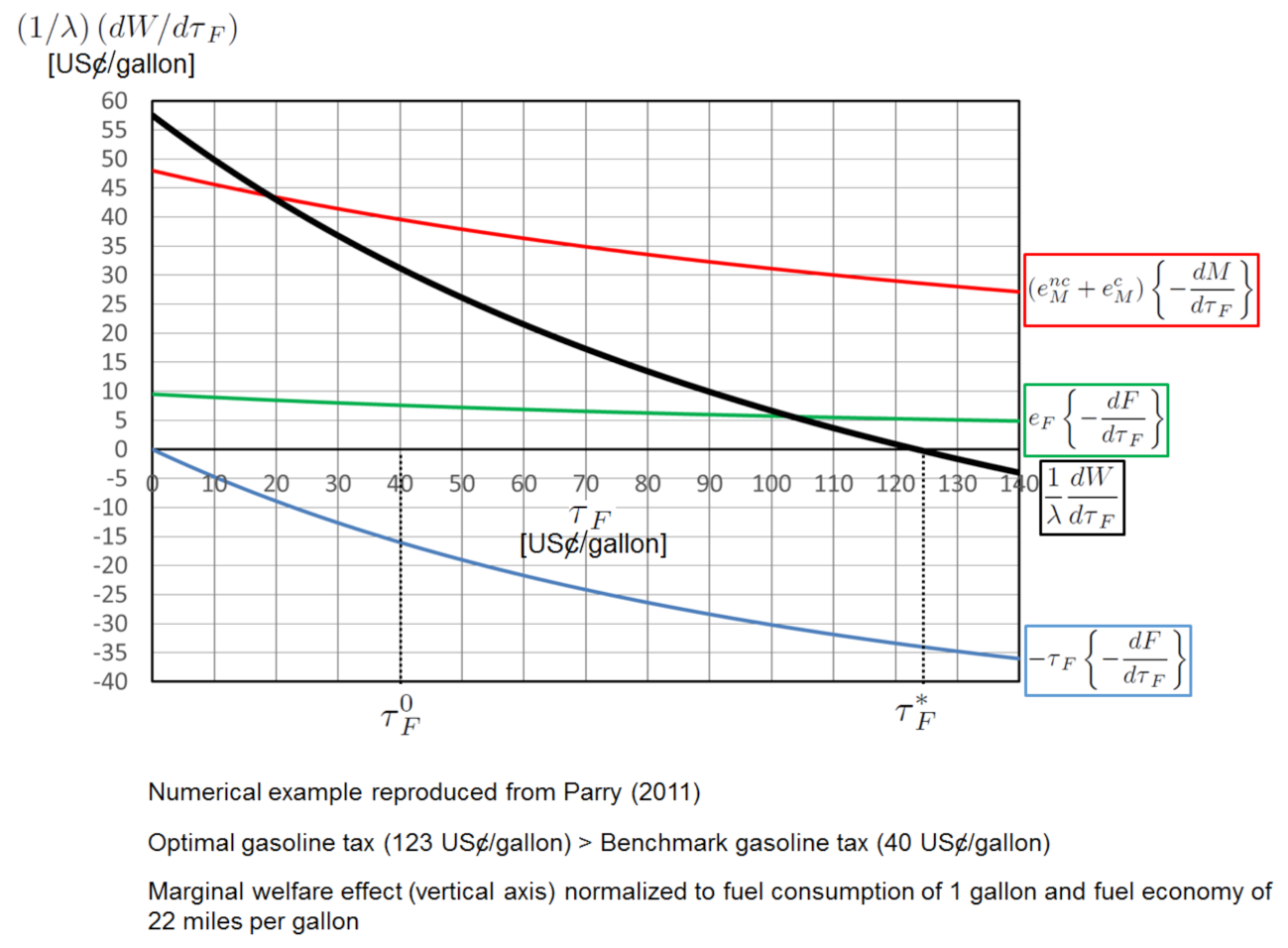
  41. Parry, I.W.H. How much should highway fuels be taxed? In US Energy Tax Policy, 1st ed.; Metcalf, G.E., Ed.; Cambridge University Press: New York, NY, USA, 2011; pp. 269–297. [Google Scholar]
  42. Tscharaktschiew, S. Shedding light on the appropriateness of the (high) gasoline tax level in Germany. Econ. Transp. 2014, 3, 189–210. [Google Scholar] [CrossRef]
  43. Tscharaktschiew, S. How much should gasoline be taxed when electric vehicles conquer the market? An analysis of the mismatch between efficient and existing gasoline taxes under emerging electric mobility. Transp. Res. Part D Transp. Environ. 2015, 39, 89–113. [Google Scholar] [CrossRef]
  44. Lin, C.-Y.C.; Prince, L. The optimal gas tax for California. Energy Policy 2009, 37, 5173–5183. [Google Scholar] [CrossRef] [Green Version]
  45. Wangsness, P.B. How to road price in a world with electric vehicles and government budget constraints. Transp. Res. Part D Transp. Environ. 2018, 65, 635–657. [Google Scholar] [CrossRef]
  46. West, S.E.; Williams, R.C., III. Optimal taxation and cross-price effects on labor supply: Estimates of the optimal gas tax. J. Public Econ. 2007, 91, 593–617. [Google Scholar] [CrossRef]
  47. Hirte, G.; Tscharaktschiew, S. The role of labor-supply margins in shaping optimal transport taxes. Econ. Transp. 2020, 22, 100156. [Google Scholar] [CrossRef]
  48. Parry, I.W.H. How should heavy-duty trucks be taxed? J. Urban Econ. 2008, 63, 651–668. [Google Scholar] [CrossRef]
  49. Parry, I.W.H.; Strand, J. International fuel tax assessment: An application to Chile. Environ. Dev. Econ. 2012, 17, 127–144. [Google Scholar] [CrossRef] [Green Version]
  50. Antón-Sarabia, A.; Hernández-Trillo, F. Optimal gasoline tax in developing, oil-producing countries: The case of Mexico. Energy Policy 2014, 67, 564–571. [Google Scholar] [CrossRef]
  51. Bösch, P.M.; Becker, F.; Becker, H.; Axhausen, K.W. Cost-based analysis of autonomous mobility services. Transp. Policy 2018, 64, 76–91. [Google Scholar] [CrossRef]
  52. Nazari, F.; Noruzoliaee, M.; Mohammadian, A.K. Shared versus private mobility: Modeling public interest in autonomous vehicles accounting for latent attitudes. Transp. Res. Part C Emerg. Technol. 2018, 97, 456–477. [Google Scholar] [CrossRef]
  53. Wadud, Z.; Chintakayala, P.K. To own or not to own—That is the question: The value of owning a (fully automated) vehicle. Transp. Res. Part C. Emerg. Technol. 2021, 123, 102978. [Google Scholar] [CrossRef]
  54. Wadud, Z.; Mattioli, G. Fully automated vehicles: A cost-based analysis of the share of ownership and mobility services, and its socio-economic determinants. Transp. Res. Part A Policy Pract. 2021, 151, 228–244. [Google Scholar] [CrossRef]
  55. Chen, S.; Wang, H.; Meng, Q. Optimal purchase subsidy design for human-driven electric vehicles and autonomous electric vehicles. Trans. Res. Part C Emerg. Technol. 2020, 116, 102641. [Google Scholar] [CrossRef]
  56. Wu, J.; Liao, H.; Wang, J.W.; Chen, T. The role of environmental concern in the public acceptance of autonomous electric vehicles: A survey from China. Transp. Res. Part F Traffic Psychol. Behav. 2019, 60, 37–46. [Google Scholar] [CrossRef]
  57. Small, K.A. Valuation of travel time. Econ. Transp. 2012, 1, 2–14. [Google Scholar] [CrossRef]
  58. Hayashi, Y.; Kato, H.; Teodoro, R.V.R. A model system for the assessment of the effects of car and fuel green taxes on CO2 emission. Transp. Res. Part D Transp. Environ. 2001, 6, 123–139. [Google Scholar] [CrossRef]
  59. Santos, G.; Behrendt, H.; Maconi, L.; Shirvani, T.; Teytelboym, A. Part I: Externalities and economic policies in road transport. Res. Transp. Econ. 2010, 28, 2–45. [Google Scholar] [CrossRef]
  60. Ostermeijer, F.; Koster, H.; van Ommeren, J.; Nielsen, V.M. Automobiles and urban density. J. Econ. Geogr. 2022. [Google Scholar] [CrossRef]
  61. Pons-Rigat, A.; Proost, S.; Turró, M. Workplace parking policies in an agglomeration: An illustration for Barcelona. Econ. Transp. 2020, 24, 100194. [Google Scholar] [CrossRef]
  62. Gabbe, C.J.; Manville, M.; Osman, T. The opportunity cost of parking requirements: Would Silicon Valley be richer if its parking requirements were lower? J. Transp. Land Use 2021, 14, 277–301. [Google Scholar] [CrossRef]
  63. Onishi, A.; Cao, X.; Ito, T.; Shi, F.; Imura, H. Evaluating the potential for urban heat-island mitigation by greening parking lots. Urban For. Urban Green. 2010, 9, 323–332. [Google Scholar] [CrossRef]
  64. Bunten, D.M.; Rolheiser, L. People or parking? Habitat Int. 2020, 106, 102289. [Google Scholar] [CrossRef]
  65. Geroliminis, N. Cruising-for-parking in congested cities with an MFD representation. Econ. Transp. 2015, 4, 156–165. [Google Scholar] [CrossRef]
  66. Inci, E.; van Ommeren, J.N.; Kobus, M. The external cruising costs of parking. J. Econ. Geogr. 2017, 17, 1301–1323. [Google Scholar] [CrossRef] [Green Version]
  67. Shoup, D.C. Cruising for parking. Transp. Policy 2006, 13, 479–486. [Google Scholar] [CrossRef]
  68. Van Ommeren, J.; McIvor, M.; Mulalic, I.; Inci, E. A novel methodology to estimate cruising for parking and related external costs. Transp. Res. Part B Methodol. 2021, 145, 247–269. [Google Scholar] [CrossRef]
  69. Chester, M.; Fraser, A.; Matute, J.; Flower, C.; Pendyala, R. Parking infrastructure: A constraint on or opportunity for urban redevelopment? A study of Los Angeles County parking supply and growth. J. Am. Assoc. 2015, 81, 268–286. [Google Scholar] [CrossRef]
  70. Molenda, I.; Sieg, G. Residential parking in vibrant city districts. Econ. Transp. 2013, 2, 131–139. [Google Scholar] [CrossRef] [Green Version]
  71. Khayati, Y.; Kang, J.E.; Karwan, M.; Murray, C. Household use of autonomous vehicles with ride sourcing. Transp. Res. Part C Emerg. Technol. 2021, 125, 102998. [Google Scholar] [CrossRef]
  72. Khayati, Y.; Kang, J.E.; Karwan, M.; Murray, C. Household Activity Pattern Problem with Autonomous Vehicles. Netw. Spat. Econ. 2021, 21, 609–637. [Google Scholar] [CrossRef]
  73. Simoni, M.D.; Kockelman, K.M.; Gurumurthy, K.M.; Bischoff, J. Congestion pricing in a world of self-driving vehicles: An analysis of different strategies in alternative future scenarios. Transp. Res. Part C Emerg. Technol. 2019, 98, 167–185. [Google Scholar] [CrossRef] [Green Version]
  74. Cutter, W.B.; Franco, S.F. Do parking requirements significantly increase the area dedicated to parking? A test of the effect of parking requirements values in Los Angeles County. Transp. Res. Part A Policy Pract. 2012, 46, 901–925. [Google Scholar] [CrossRef] [Green Version]
  75. Davis, L.W.; Knittel, C.R. Are fuel economy standards regressive? J. Assoc. Environ. Resour. Econ. 2019, 6, S37–S63. [Google Scholar] [CrossRef] [Green Version]
  76. De Borger, B.; Proost, S. Traffic externalities in cities: The economics of speed bumps, low emission zones and city bypasses. J. Urban Econ. 2013, 76, 53–70. [Google Scholar] [CrossRef]
  77. Nie, Y.M. On the potential remedies for license plate rationing. Econ. Transp. 2017, 9, 37–50. [Google Scholar] [CrossRef] [Green Version]
  78. Nitzsche, E.; Tscharaktschiew, S. Efficiency of speed limits in cities: A spatial computable general equilibrium assessment. Transp. Res. Part A Policy Pract. 2013, 56, 23–48. [Google Scholar] [CrossRef]
  79. Tscharaktschiew, S. Why are highway speed limits really justified? An equilibrium speed choice analysis. Transp. Res. Part B Methodol. 2020, 138, 317–351. [Google Scholar] [CrossRef]
  80. Cascetta, E.; Cartenì, A.; Di Francesco, L. Do autonomous vehicles drive like humans? A Turing approach and an application to SAE automation Level 2 cars. Transp. Res. Part C Emerg. Technol. 2022, 134, 103499. [Google Scholar] [CrossRef]
  81. Gkartzonikas, C.; Gkritza, K. What have we learned? A review of stated preference and choice studies on autonomous vehicles. Transp. Res. Part C Emerg. Technol. 2019, 98, 323–337. [Google Scholar] [CrossRef]
  82. Bansal, P.; Kockelman, K.M.; Singh, A. Assessing public opinions of and interest in new vehicle technologies: An Austin perspective. Transp. Res. Part C Emerg. Technol. 2016, 67, 1–14. [Google Scholar] [CrossRef]
  83. Bansal, P.; Kockelman, K.M. Are we ready to embrace connected and self-driving vehicles? A case study of Texans. Transportation 2018, 45, 641–675. [Google Scholar] [CrossRef]
  84. Daziano, R.A.; Sarrias, M.; Leard, B. Are consumers willing to pay to let cars drive for them? Analyzing response to autonomous vehicles. Transp. Res. Part C Emerg. Technol. 2017, 78, 150–164. [Google Scholar] [CrossRef] [Green Version]
  85. Cartenì, A. The acceptability value of autonomous vehicles: A quantitative analysis of the willingness to pay for shared autonomous vehicles (SAVs) mobility services. Transp. Res. Interdiscipl. Perspect. 2020, 8, 100224. [Google Scholar] [CrossRef]
  86. Becker, F.; Axhausen, K.W. Literature review on surveys investigating the acceptance of automated vehicles. Transportation 2017, 44, 1293–1306. [Google Scholar] [CrossRef] [Green Version]
  87. Wali, B.; Santi, P.; Ratti, C. Modeling consumer affinity towards adopting partially and fully automated vehicles—The role of preference heterogeneity at different geographic levels. Transp. Res. Part C Emerg. Technol. 2021, 129, 103276. [Google Scholar] [CrossRef]
  88. Elvik, R. The demand for automated vehicles: A synthesis of willingness-to-pay surveys. Econ. Transp. 2020, 23, 100179. [Google Scholar] [CrossRef]
  89. Sheela, P.V.; Mannering, F. The effect of information on changing opinions toward autonomous vehicle adoption: An exploratory analysis. Int. J. Sustain. Transp. 2020, 14, 475–487. [Google Scholar] [CrossRef]
  90. Liu, P.; Guo, Q.; Ren, F.; Wang, L.; Xu, Z. Willingness to pay for self-driving vehicles: Influences of demographic and psychological factors. Transp. Res. Part C Emerg. Technol. 2019, 100, 306–317. [Google Scholar] [CrossRef]
Figure 1. Example of the marginal welfare effect of the gasoline tax and optimal gasoline tax (reproduced from [41]).
Futuretransp 02 00019 g001
Figure 2. Optimal transport tax.
Futuretransp 02 00019 g002
Figure 3. Stepwise change in optimal transport taxes owing to self-driving cars.
Futuretransp 02 00019 g003
Table 1. Related Literature.
StudyInstrumentRegion
Parry and Small (2005) [8]Gasoline tax, Miles taxUS, UK
Santos (2017) [9]Gasoline tax, Diesel taxVarious European countries
Parry and Timilsina (2010) [40]Gasoline tax, Miles taxMexico City
Parry (2011) [41]Gasoline tax, Diesel tax (heavy-duty trucks)US
Tscharaktschiew (2014) [42]Gasoline taxGermany
Tscharaktschiew (2015) [43]Gasoline tax (with EV substitution)Germany
Lin and Prince (2009) [44]Gasoline taxCalifornia
Wangsness (2018) [45]Kilometer tax (peak, off-peak)Norway (urban, rural)
West and Williams (2007) [46]Gasoline tax 1 US
Hirte and Tscharaktschiew (2020) [47]Gasoline tax, Miles tax 1 US, UK
Parry (2008) [48]Diesel tax (heavy-duty trucks)US
Parry and Strand (2012) [49]Gasoline tax, Diesel tax (commercial trucks)Chile
Antón-Sarabia and Hernández-Trillo (2014) [50]Gasoline taxMexico
1 Focus on the role of labor supply.
Table 2. Notational glossary.
NotationDescription
UUtility
XGeneral consumption
LLeisure
vVehicle stock of the household
mVehicle mileage per traveler (occupied trips)
MVehicle mileage per household (occupied trips)
tTravel time per mile
TAggregate travel time of the household
fFuel/energy consumption per mile
FAggregate fuel/energy consumption of the household
EExternality index
p F Fuel/energy price
p X Price of the composite commodity
τ F Fuel/energy tax
c ( f ) Costs of car ownership not related to energy consumption
IHousehold labor income
G O V Revenue recycling instrument of the government (tax or transfer)
Γ Total time endowment of the household
λ Marginal utility of monetary household income
θ Value of travel time
e F Marginal external cost of fuel/energy consumption
e M Marginal external cost of vehicle mileage
WWelfare
Ω Set of parameters exogenous to the household
ϕ Parking requirement per vehicle
PParking requirement per household
nDriverless vehicle mileage per traveler (unoccupied trips)
NDriverless vehicle mileage per household (unoccupied trips)
Publisher’s Note: MDPI stays neutral with regard to jurisdictional claims in published maps and institutional affiliations.

