Application of Machine Learning Classifiers for Mode Choice Modeling for Movement-Challenged Persons

Abstract

In this study, we aimed to evaluate the performance of various machine learning (ML) classifiers to predict mode choice of movement-challenged persons (MCPs) based on data collected through a questionnaire survey of 384 respondents in Dhaka, Bangladesh. The mode choice set consisted of CNG-driven auto-rickshaw, bus, walking, motorized rickshaw, and non-motorized rickshaw, which was found as the most prominent mode used by MCPs. Age, sex, income, travel time, and supporting instrument (as an indicator of the level of disability) utilized by MCPs were explored as predictive variables. Results from the different split ratios with 10-fold cross-validation were compared to evaluate model outcomes. A split ratio of 60% demonstrates the optimum accuracy. It was found that Multi-nominal Logistic Regression (MNL), K-Nearest Neighbors (KNN), and Linear Discriminant Analysis (LDA) show higher accuracy for the split ratio of 60%. Overfitting of bus and walking as a travel mode was found as a source of classification error. Travel time was identified as the most important factor influencing the selection of walking, CNG, and rickshaw for MNL, KNN, and LDA. LDA and KNN depict the supporting instrument as a more important factor in mode choice than MNL. The selection of rickshaw as a mode follows a relatively normal probability distribution, while probability distribution is negatively skewed for the other three modes.

1. Introduction

Transportation mode choice is an integral part of a trip-making process. Transportation planners model the mode choice decision to predict the travel demand and understand the causal factors influencing mode choice in order to undertake more pragmatic, efficient, and sustainable transportation policies [1]. Traditionally, analysis of mode choice of individuals in travel behavior research is widely supported by discrete choice models based on the principles of utility maximization, i.e., trip makers will select the mode with the highest utility [2]. Discrete choice models are most notably based on logit models, such as the multinomial logit model and the nested logit model [1,2]. However, logit models have a solid mathematical and statistical foundation that requires input data to fulfill a number of assumptions, e.g., that the probability of selection of a travel mode should be independent of the attributes of other alternate travel modes [3]. Machine learning (ML) techniques are nonparametric, and aim to determine the underlying pattern within the data instead of making assumptions regarding the data; hence, ML techniques are flexible in nature. ML tools evaluate the complex relationships among variables in a more prudent way by diving them into the accuracy of the predictions, sources of error in prediction, the relative significance of factors influencing a phenomenon, probability of occurrence of a phenomenon, etc. [4,5,6].

In recent years, there has been a growing interest in applying ML methods to model individual choice behavior. ML tools have been used in different fields of transportation planning: mode choice behavior, accident analysis, traffic safety, and traffic signal control in studies, and in most cases, it has been found that ML outperforms logit models [5,6,7,8]. ML methods have been applied for modeling mode choice for freight transport [9], home-based trips for individuals [4,8,10], commuters’ mode choice [11], school trips [12], and location-based social networks to understand human mobility and people’s behaviors by mining check-in patterns [13,14]. Based on the literature, no study has yet been conducted to exclusively explore the mode choice of persons with a disability (PWDs) using ML techniques. Although there are studies regarding mobility patterns and travel behavior of persons with a disability using different logistic regression and participatory methods [15,16,17,18,19], rarely has any study focused on the application of ML classifiers for analyzing the travel behavior of PWDs (PWDs are people with physical or cognitive impairment. PWDs include people with deformity in the leg or hand, mental instability, blindness, or an inability to hear).In this study, we aimed to address this gap in the literature by applying various ML classification techniques to analyze the mode choice of mobility-challenged persons (MCPs), a group of persons with an impairment in their legs who depend on a wheelchair, walking frame, crutch, and/or cane for their movement [20], in Dhaka, Bangladesh. We developed different ML models/codes to predict the mode choice of MCPs with relevant factors as predictors (as discussed in the next paragraph) as a maiden approach to explain mode choice of PWDs using ML. We compared ML models to determine whether there was a significant difference between the performance of ML techniques and identified which ML techniques performed more efficiently in predicting mode choice of MCPs in Dhaka.

Literature reveals that socio-demographics such as age, sex, travel time, and income are significant factors influencing mode choice. Elderly people prefer to travel in a comfortable, safe, and convenient mode [21,22]. Likewise, women prefer to choose a comfortable, convenient, and safe mode [23]. Both elderly people and women are considered to be not as physically strong as younger or middle-aged people and males, respectively. As a result, they prefer to travel by a transport mode which will minimize physical exertion. For this, elderly people and women are less inclined to walk and prefer other modes of transport [21]. Monthly income is an important determinant of mode choice. People with higher income have greater financial means and a higher propensity to travel by modes with relatively higher travel cost [24]. Upper-income households and individuals are thought to place a higher value on the comfort and convenience associated with the private car [25]. Travel time is another very significant factor, as people usually prefer to travel by a mode that will minimize their travel time. People generally prefer to travel by motorized means such as bus or car when distances are farther, but walking is preferred for shorter distances of travel [3,26,27,28].

Along with the previously described factors, supporting instrument (walking frame, cane, crutch, wheelchair) as a disability-related parameter can play a large role in the selection of mode choice for MCPs. For example, Frey (2013) found that wheelchair users are more reluctant to travel by bus than crutch or cane users in developing countries [17]. Based on the literature review, age, sex, income, supporting instrument, and travel time for regular trips are considered as predictor variables to model the mode choice of MCPs. However, there is a dearth of research focusing on the mobility challenges faced by MCPs in megacities in developing countries. Therefore, it is necessary to understand the problems of the transportation system that MCPs face in selecting their travel mode using a study area from a developing country.

In this study, we aimed to investigate mode choice of MCPs using ML methods based on data collected through questionnaire surveys. We first describe the ML tools used in this study, then explore the parameters and cross-validation methods used for evaluating the performance of the classifiers. Findings from the study are presented. In the result section, along with the performance of the model, the relative importance of the considered factors (including disability parameter) influencing mode choice are explored. Hopefully, the findings of the study will provide effective insight to develop pragmatic policy measures to ensure sustainable mobility for MCPs and provide relevant recommendations in this regard.

2. Study Area

Dhaka, the capital city of Bangladesh, was selected as the study area. Dhaka is the 11th megacity in the world, with a population of 20 million [29]. According to World Bank (2018), more than 1 million PWDs are living in Dhaka city [30]. Literature reveals that it is very common for PWDs in Dhaka to face mobility challenges due to the unfriendly nature of transportation modes and pedestrian infrastructures [31,32] and a lack of awareness among transportation workers about the mobility rights of PWDs [33,34,35]. Nonetheless, the struggle faced by the PWDs regarding mobility in the megacity is mostly invisible, and overshadowed by the other problems in the transport sector of the city. A number of empirical studies have shed light on the inaccessibility of transportation systems for MCPs in Dhaka [30,33,34]. Due to the presence of a large number of PWDs (including MCPs) and poor accessibility of the transportation system for PWDs, Dhaka was selected as the case study area for the research, as it is an ideal city to examine the mode choice of MCPs in a disadvantaged situation and explore the influence of mobility challenges on mode choice.

3. Data for the Study

A total of 400 MCPs from Dhaka city were selected as samples for the study using the Convenience Sampling Method. A paper-based questionnaire interview was conducted. The survey was conducted at rehabilitation centers and orthopedic departments of several hospitals, as MCPs are likely to visit these places for their medical treatment. Selected survey locations were the Centre for Rehabilitation for the Paralyzed, Bangabandhu Sheikh Mujib Medical University, the Physically Challenged Development Foundation, and the National Grass-root Disable Organization. Each of these institutions granted permission to survey their constituents, and all MCPs surveyed consented to take part in the study. However, as MCPs were not always eager to share their mobility-related data owing to privacy concerns, the sample size was limited to 400 participants. A brief description of the respondents is provided in

Table 1. A brief overview of the stratification of samples and ordinal scaling of factors.

Factor and Categories	Percentage	Factor and Categories	Percentage
Sex		Income
Male	45.4%	<25,000 BDT (Lower income)	33.4%
Female	54.6%	25,000–50,000 BDT (Middle income)	47.3%
		>50,000 BDT (Higher-income)	19.3%
Age		Mobility aid
0–25 years (Young)	25.8%	Wheelchair	31.8%
25–50 years (Middle Aged)	41%	Walking Frame/Crutch	34.3%
Greater than 50 years (Elderly people)	33.2%	Walking Stick	34%

. In the survey, MCPs were asked to provide information regarding mode choice for regular trips, age, sex, income, car ownership, travel time, and supporting instrument used.

4. Machine Learning Classifiers

In this section, classification methods used in the study are described in brief, and information about the calibration process of the classifier is provided. The following ML techniques were employed in the current study, as they are widely used in transportation mode choice modelling (

Table 2. Minimum sample requirement for different ML methods and their application in mode choice modelling.

ML Techniques	Procedure for Determining Minimum Number of Samples	Required Number of Samples for This Study	Literature on Particular ML Technique Used for Mode Choice Modelling
Multi-nominal logistic (MNL) regression	10 cases per predictor [36]	10 × 5 = 50	[4,6,8,9]
Naïve Bayes (NB)	Naïve Bayes can be applied on relatively smaller size of samples. Chen et al. (2021) found that when the sample is less than 400 and the number of categories is less than 24, naïve Bayes shows a satisfactory accuracy [15]	As Naïve Bayes works for small sample sizes and the literature testifies, 384 samples will be sufficient	[6,9,37]
Linear Discriminant Analysis (LDA)	Number of samples must be larger than number of predictors [38]	No of samples 384 which is greater than no of predictors 5.	[8,39]
Random Forest (RF)	Random Forest can be applied to a smaller number of samples. Scholarly articles reveal RF can be applied on a relatively smaller number of samples for classification. Farhadian et al. (2020) applied RF on 356 samples and received satisfactory peformance [40]	384 samples will be sufficient	[4,9,41]
Neural Network (Nnet)	50 times more than the number of independent variables [42]	Number of required samples 50 × 5 = 250	[4,9,13]
K-Nearest Neighbor (KNN)	Classification of features in KNN depends on distance between data points instead of number of samples [43,44]	384 samples will be sufficient	[9,37]
Gradient Boosting	It can be applied to a dataset as small as 100 samples [45]	384 samples will be sufficient	[4,9,45]

). According to the literature, these models are suitable to develop predictive models with as little as 50 samples.

• Multi-nominal logistic (MNL) regression
• Naïve Bayes (NB)
• Linear Discriminant Analysis (LDA)
• Random Forest (RF)
• Neural Network (Nnet)
• K-Nearest Neighbor (KNN)
• Gradient Boosting

In this study, multi-nominal logistic regression (MNL) is used to determine the probability of selecting a transportation mode, using the logistic function to minimize the pertaining cost function. Likewise, discrete choice model, MNL is fit using maximum likelihood estimation [4].

Naïve Bayes (NB) function is based on the Bayes theorem and follows a conditional probability model. The inherent assumption of NB is that every pair of features is independent. It classifies the outcome following a supervised learning technique. NB requires only a small amount of data to develop the model. To calculate the probability of mode selection, it was assumed that mode choice followed a Gaussian distribution [4,10].

Linear discriminant analysis (LDA) is a method used to find a linear combination of features that characterizes or separates two or more classes of objects or events. The LDA technique is widely used for solving problems with a small sample size [38].

Neural network (Nnet) is akin to biological neurons, where neurons or nodes are connected to form a network. Neural network transforms input features through hidden layers to effectively model the outputs with due consideration of complex interaction and structures within the data. The backpropagation algorithm was used to allocate weight to each layer [4,7]. The number of hidden layers considered for this study was three.

Random Forest (RF) is an ensemble classification method that operates by creating multiple decision trees during the training phase. The key difference between RF and a decision tree is that decision trees only consider the best split for all variables at each node, while RF develops a collection of trees in a random manner. These trees grow by the addition of random elements, i.e., by the selection of few variables in a random combination by the algorithm. Each tree makes its own prediction, and the most voted classification is selected as the final output by the algorithm. The sample size for a random forest acts as a control on the degree of randomness. Increasing the sample size results in a less random forest, which may lead to overfit. Decreasing the sample size increases the variation in the individual trees within the forest, preventing overfitting, but negatively influences model performance. A useful side effect is that lower sample sizes reduce the time needed to train the model. In comparison to Decision Tree, RF is more well-suited for a relatively smaller sample size. Random Forest can consider several to thousands of trees to build the model. In this study, 1000 trees were considered for RF classification [4,5,9,41].

K-Nearest Neighbor (KNN) is an unsupervised learning algorithm based on the k training examples within the closest distance of each query point. KNN classifies the query point based on the closest neighbors of each point [4,9]. In this study, the value of k was considered to be 10.

Gradient Boosting is an ensemble meta estimator of weak prediction models, typically decision trees, which are widely used for classification. Classes are predicted by the algorithm in terms of the majority vote of the weak learners’ predictions weighted based on respective accuracy rates. It can be applied on a small sample (such as 100–1000) [45,46].

The R packages used in developing ML models and algorithms are: foreign [47], reshape2 [48], caret [49], pdp [50], neuralnet [51], gbm [52], MASS [53], cvms [54], tibble [55], class [56], CaTools [57], and ISLR [58].

5. Comparison of Models

A combination of k fold cross-validation and the holdout method was used to compare the classification models using software R 4.0.2 version [59]. There is not sufficient research on the suitable split ratio between training and test data and how the split ratio influences the predictive capability of the model. A common practice is to split the data into a 2:1 ratio. However, it is never guaranteed that a 2:1 split ratio (training set > test set) will provide the best result [60]. For this, we replicated a number of split ratios of the dataset and evaluated the performance of the model empirically.

At first, the data was divided into Training Set (TRS) and Test Set (TSS) for a split ratio of 0.1, 0.2, 0.3, and 0.4 for test data maintaining the condition of TRS > TSS. Next, TRR was subjected to k-fold cross-validation to randomly partition the TRS into k disjoint subsets. K-fold cross-validation utilizes (k-1) sets from the TRS to train the model and the rest one subset (kth) of the TSS is used to test the model. For different k values and split ratios, the performance of the classifiers was evaluated. Then, the models were estimated based all of the training data. Later, these models were applied to the testing dataset to predict the mode choice [9]. The developed model was applied on the TSS to evaluate the predictive capacity of the model in terms of accuracy, F1 score, recall, and kappa [61].

Accuracy, precision, kappa, recall, and F1 score are the most commonly used parameters to evaluate performance of ML models [4,62,63,64,65,66], and these parameters have been employed to assess performance of each of the ML models of mode choice in this study.

Accuracy (A): Accuracy is the percentage of observations classified accurately in a dataset. Accuracy is determined by the number of correctly classified observations divided by the total number of observations used for classification.

Precision (P): Precision is the ratio of correctly classified observations to the total number of retrieved instances for a similar class in the dataset. It is also well-known as positive predictive value [64]. Precision is calculated by dividing the total number of predicted accurate classes by the total number of actual observations for that class.

Kappa: Cohen’s kappa (k) is a metric used to determine inter-reliability and intra-rater reliability between observed and predicted data. Kappa considers the probability of agreement occurring by chance. Values of kappa from 0 to less than 0.2, 0.21–0.4, 0.41–0.6, 0.61–0.8, and 0.81–1.00 represent no agreement, slight agreement, fair agreement, substantial agreement, and almost perfect agreement, respectively. Kappa (k) is calculated as below:

K = (po − pe)/(1 − pe)

where po equals relative observed agreement among raters and pe equals the hypothetical probability of chance agreement calculated using the observed data.

Four metrics, accuracy, precision, recall, and F1-score, are used to evaluate the performance of the models based on the confusion matrix generated by the model [65].

Recall (R): Recall measures the fraction of the observation belonging to a particular class that has been particularly classified properly by the model. Recall is also called sensitivity. It is determined by dividing correctly classified observations for a class by the total number of actual observations predicted for that class by the model [66].

F1-score (FS): F1-score is the harmonic mean of precision and recall. While precision and recall consider only false positive and false negative, respectively, F1-score considers both. F1 is very useful when class distribution is uneven [63].

$$\mathrm{FS}=\frac{2\mathrm{x} \mathrm{P}\ast \mathrm{R}}{\mathrm{P}+\mathrm{R}}$$

Assume that we have two modes X and Y, and the total number of observations is 50. A ML method has correctly classified 20 mode X observations as mode X, 10 mode X observations as mode Y, 5 mode Y observations as mode X, and 15 mode Y observations as mode Y (

Table 3. A hypothetical scenario calculating comparison parameters of classifiers.

Observed	Predicted		Total
	X	Y
X	20 (XX)	10 (XY)	30
Y	5 (YX)	15 (YY)	20
Total	25	25	50 (T)

).

Accuracy of the model = (XX + YY)/T = [(20 + 15)/100] = 0.7;

Precision for mode X, PX = XX/(XX + XY) = 20/25 = 0.8;

Recall for mode X, RX = XX/(XX + YX) = 20/30 = 0.67; and

F1-score for mode X, FX = 2 × PX × RX/(PX + RX) = [2 × (0.8 × 0.67)]/(0.8 + 0.67) = 0.73

To calculate kappa, agreement between predicted and observed data is identified. Here we have agreement of X predicted as 20 and Y predicted as 15.

Observed proportionate agreement

Po = (20 + 15)/50 = 0.7

Probability of predicting X px = [(XX + XY)/T] × [(XX + YX)/T] = (25/50) × (30/50) = 0.30

Probability of predicting Y py = [(YY + XY)/T] × [(YY + YX)/T] = (25/50) × (20/50) = 0.20

Overall agreement of X or Y is pe = px + py = 0.30 + 0.20 = 0.50

K = (po − pe)/(1 − pe) = (0.7 − 0.5)/(1 − 0.5) = 0.4

6. Data Analysis and Results

After analyzing these data, it was found that the primary mode choice for regular trips of MCPs comprises bus, walking, rickshaw, and compressed natural gas (CNG)-driven auto-rickshaw (locally known as CNG). The rickshaw, a tricycle pulled by a person, was found to be the most prominent mode (45%) used by MCPs, while22% of the MCPs were found to use the CNG auto-rickshaw, a gas-driven vehicle, for regular trips. The percentage of MCPs depending on walking on a regular trip with the support of a wheelchair or other walking instruments was 16%. The percentage of MCPs using the bus (including minibuses) was considerably lower (14%). Considering the challenges faced by PWDs to board buses which are lacking wheelchair ramps and the overcrowded nature of the buses of Dhaka city, it is likely that MCPs will have less inclination to travel by bus [67,68]. Car transportation covers only 4% of the mode share of MCPs.

It was found that car-user MCPs have a much higher dependence on cars, as MCPs who own a car did not use any other modes. However, bus-, rickshaw-, CNG-, and walking-dependent MCPs were found to use alternative modes in addition to their regular mode of travel. As the choice of car as a travel mode of MCPs was determined only by car ownership, MCPs using cars were not considered for ML classification, leading to a reduced total sample of 384.

As the supporting instrument was a nominal variable, it was converted to an ordinal variable for data analysis. The severity of disability was dependent upon the physical capability to transfer body weight to the legs, which helps to determine movement-supporting instruments used by MCPs by medical professionals. The wheelchair is recommended to persons who can put the least amount of weight on their legs or are not capable of using their leg(s) to walk. Canes are recommended to MCPs whose lower limbs can tolerate a relatively higher amount of weight, and hence, they are least dependent on movement-supporting instruments. Meanwhile, walking frames and crutches are suggested to MCPs who can use their lower limbs to move from one place to another but can transfer a relatively smaller amount of weight on their legs in comparison to cane users. For this, the dependency of MCPs on supporting instruments can be considered between wheelchair and cane users [69,70]. MCPs using a wheelchair, walking frame, crutch, or cane are provided with an ordinal scale of 3, 2, or 1, respectively, representing highest, moderate, or least levels of disability. Similarly, sex is coded as female (0) or male (1).

Classification models were built using R programming software. R has several packages that allow the application of ML models. The authors report only results from k = 10 fold, as there were rarely any changes in the accuracy measures found for k = 20 and k = 30. For 10-fold cross-validation, each classification method was run for a split ratio of 0.9, 0.8, 0.7, and 0.6.

6.1. Accuracy of the Classifiers

Figure 1 reveals the maximum, minimum, and average accuracy for each classification method based on split ratios. In terms of the average accuracy, MNL was found to have the best result of 77.76%. Among the other ML techniques, LDA and KNN had the second- and third-highest average accuracy of 73.63% and 75.68%, respectively. The next best classifiers were Naïve Bayes (70.52%) and Bagging (70.10%), with average accuracies greater than 70%. Random Forrest, Neural network, and Gradient boosting had accuracies of 65.83%, 68.3%, and 65.1%, respectively. Gradient boosting was found to have the lowest average accuracy. Values of accuracy had the lowest standard deviation, with a split ratio of 0.6 across all classifiers; therefore, it was chosen as the optimal solution. As optimal ratio helps to build better prediction based on the more efficient model, a split ratio of 0.6 was used for subsequent analysis.

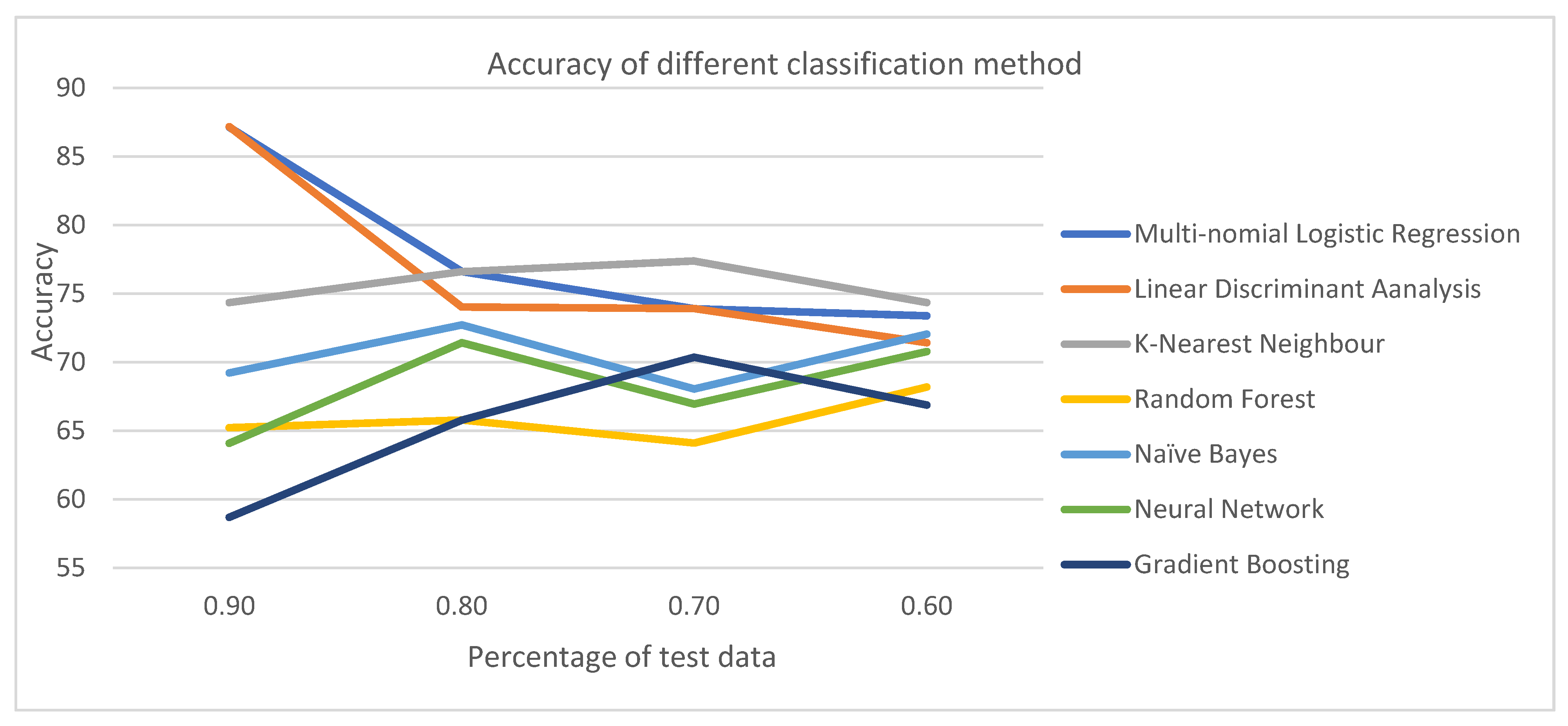
Figure 2 depicts how accuracy changes with the split ratio. Different patterns in the accuracy changes were found among classification methods. For MNL and LDA, accuracy continued to decline with the increase in testing samples. Interestingly, accuracy was enhanced when the split ratio changed from 0.9 to 0.7, but was reduced for a split ratio of 0.6 for KNN and Gradient Boosting. For RF, Naïve Bayes and Nnet accuracy were reduced when the split ratio changed from 0.9 to 0.8, increased when the split ratio was 0.7, and then were reduced when the split ratio was 0.6. Linear Discriminant Analysis had the highest range of accuracy values, followed by MNL and Gradient boosting. KNN had the lowest range of accuracy. It can be concluded that with the increase in training data, accuracy has not always increased. 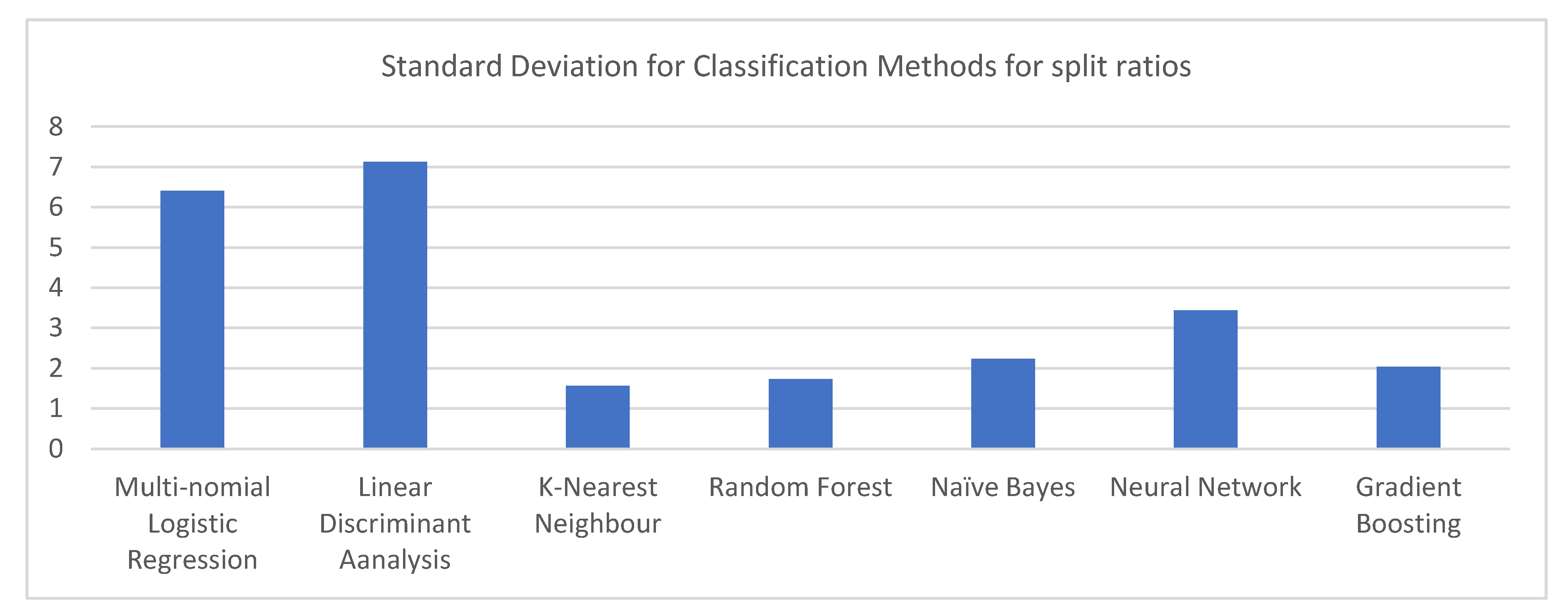Figure 3 reveals the standard deviation of the accuracy of classification methods. It was found that MNL had the highest standard deviation of accuracy and KNN had the lowest standard deviation of accuracy. It can be interpreted that the accuracy of MNL declined most with the increase in test data.

Figure 3 shows the standard deviation of the accuracy of classification methods of split ratios. KNN has the lowest standard deviation, while LDA has the highest standard deviation. This implies that with a change in training and testing samples, accuracy has changed least for KNN and most for LDA.

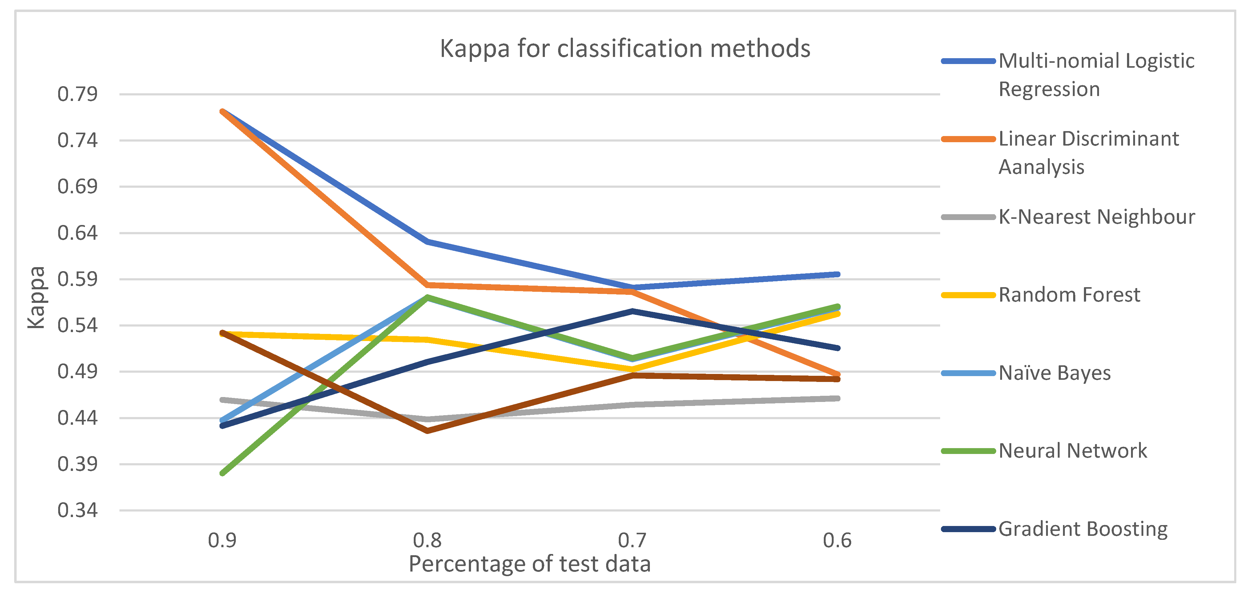
6.2. Kappa Statistics for Classifiers

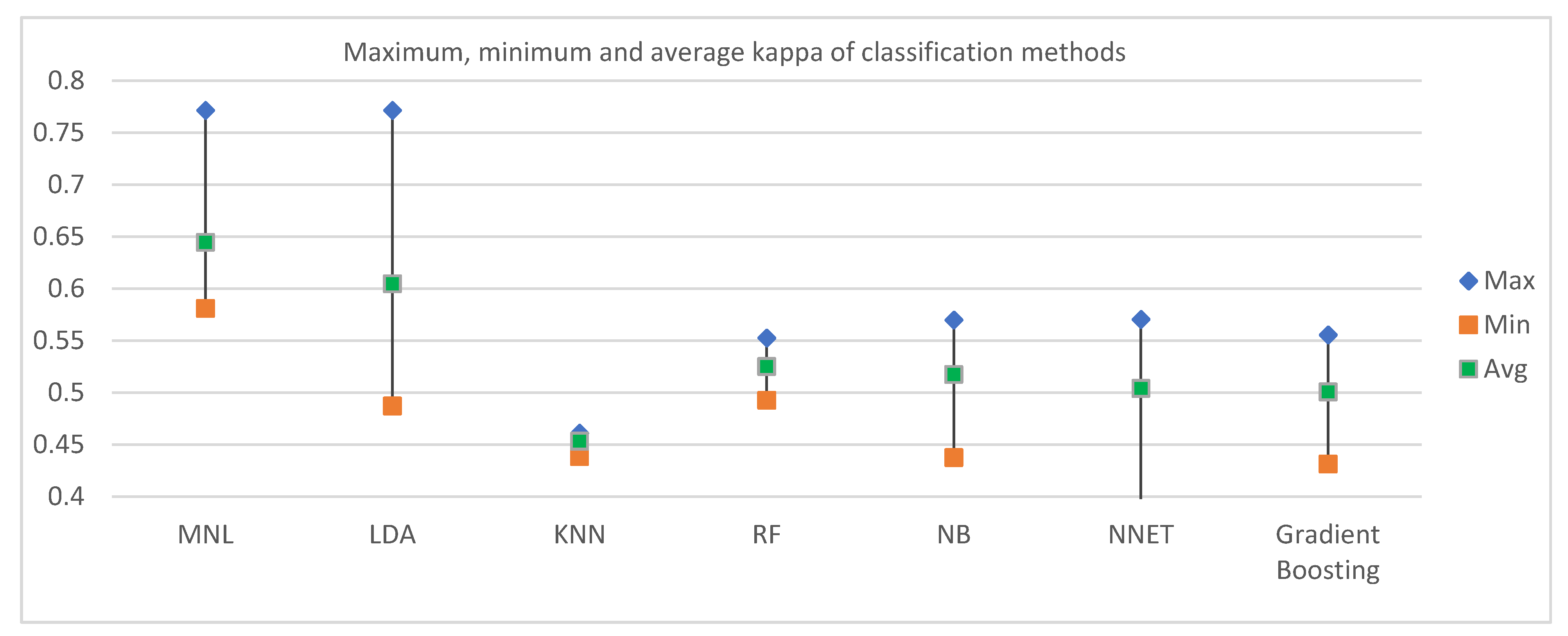
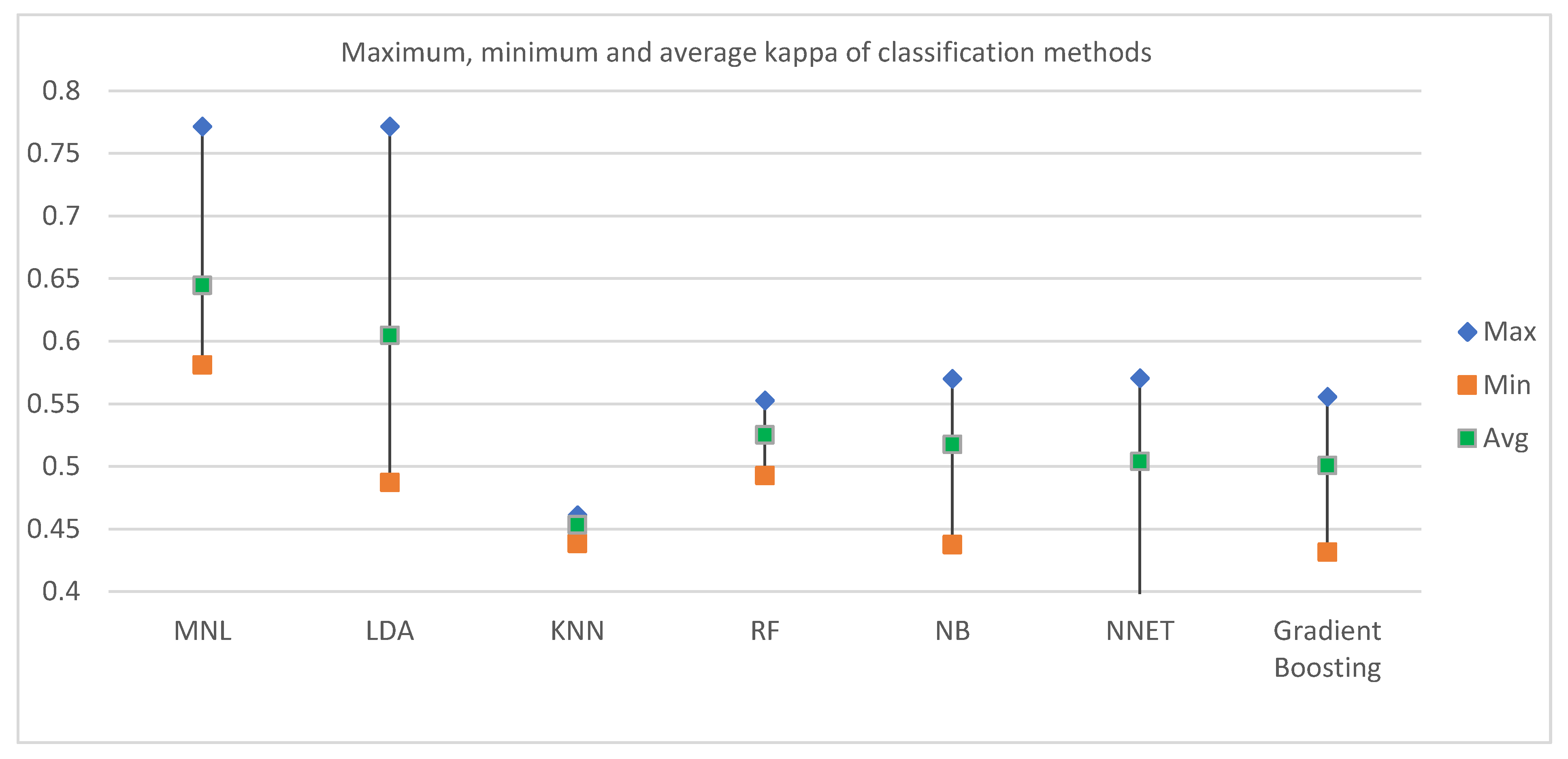
Figure 4 reveals the maximum, minimum, and average kappa for each classification method based on split ratios. In terms of the average accuracy, MNL was found to have the best result (0.644). Among the other ML techniques, LDA and RF had the second and third highest average kappa of 0.6046 and 0.5250, respectively. The next best classifiers in terms of kappa were found in Naïve Bayes and Neural Network.

Figure 5 reveals how kappa changes with the split ratio for different classification methods. The pattern of changing kappa with a split ratio varies among classification methods. MNL and RF follow similar patterns: kappa decreases with an increase in test data up to a split ratio of 0.7, and then reduces at a split ratio of 0.6. For NB and Neural Network, kappa enhances when the split ratio is changed from 0.9 to 0.8, but increases when the split ratio changes to 0.7; it later decreases again when the split ratio becomes 0.6. Kappa increases for Gradient boosting but decreases for KNN when the split ratio is changed from 0.9 to 0.8. Later Kappa continues to increase for both of the methods until the split ratio reaches 0.6.

6.3. Precision, Recall, and F-1 Score for Classifiers

Along with MNL, LDA and KNN have higher accuracy. Because of this, LDA and KNN were used for further analysis of precision, recall, and F1-score to compare with MNL. It was found that KNN had higher precession for the bus mode choice in comparison to MNL and LDA. For CNG and rickshaw, MNL was found to make a more precise prediction for all split ratios except 0.9. For walking, LDA provided a more precise prediction for split ratio 0.9, while MNL provided higher precision for split ratio 0.7. MNL and LDA simultaneously provided a higher level of precision for the split ratio of 0.8 for walking, while LDA and KNN simultaneously had higher precision for the split ratio of 0.6 for walking. It can be stated that LDA was more precise to predict walking (Table 2).

For the bus, the value of recall was found to be higher for LDA for split ratios 0.7 and 0.8.The recall value was the same for MNL, LDA, and KNN for bus for a split ratio of 0.9, and MNL and KNN for the split ratio of 0.6. For CNG, the value of recall was found to be higher for KNN for a split ratio of 0.8, while the value of recall was the same for three methods for the split ratio of 0.9, 0.7, and 0.6. Rickshaw had the highest recall for MNL for split ratio 0.9, while recall value was the same and higher for MNL and KNN, respectively, for split ratios 0.8 and 0.6. MNL and KNN had a higher recall for the rickshaw for a split ratio of 0.7. MNL and LDA had an equal and higher recall, respectively, for split ratio 0.9 for walking. These three methods had the same recall for walking for a split ratio of 0.8. For split ratios 0.6 and 0.7, highest recall was found for MNL and LDA, respectively, for walking. As MNL had the highest value of recall for three split ratios, it can be stated that LDA has a relatively higher sensitivity for walking (

Table 4. Precision, Recall, and F1-Score for MNL, LDA, and KNN.

	Classifier		MNL			LDA			KNN
Split Ratio	Modes	Precision	Recall	F-1 Score	Precision	Recall	F-1 Score	Precision	Recall	F-1 Score
0.9	Bus	0.83	0.75	0.79	0.75	0.75	0.75	1	0.75	0.86
	CNG	0.7	0.67	0.68	1	0.67	0.8	0.57	0.67	0.62
	Rickshaw	0.68	1	0.81	0.85	0.96	0.9	0.76	0.83	0.79
	Walking	0.82	0.83	0.83	1	0.83	0.91	0.75	0.5	0.6
0.8	Bus	0.89	0.62	0.73	0.86	0.46	0.6	1	0.62	0.76
	CNG	0.83	0.71	0.77	0.62	0.57	0.59	0.79	0.79	0.79
	Rickshaw	0.73	0.95	0.83	0.12	0.92	0.22	0.06	0.92	0.11
	Walking	1	0.58	0.74	1	0.67	0.8	0.83	0.42	0.56
0.7	Bus	0.75	0.44	0.55	0.73	0.5	0.59	0.89	0.44	0.59
	CNG	1	0.57	0.72	0.68	0.57	0.62	0.77	0.57	0.65
	Rickshaw	0.85	0.97	0.9	0.72	0.88	0.79	0.75	0.97	0.84
	Walking	1	0.71	0.83	0.92	0.71	0.8	0.83	0.71	0.76
0.6	Bus	0.8	0.46	0.59	0.81	0.5	0.62	0.81	0.5	0.62
	CNG	0.64	0.5	0.56	0.61	0.5	0.55	0.61	0.5	0.55
	Rickshaw	0.71	0.86	0.78	0.15	0.88	0.26	0.15	0.88	0.26
	Walking	0.83	0.89	0.86	0.91	0.71	0.8	0.91	0.71	0.8

).

KNN had the highest F1-score for split ratios 0.9 and 0.8, while LDA had the highest F1-score for split ratio 0.7 for the bus. Both LDA and KNN had a higher F1-score for a split ratio of 0.6. The highest F1-score was found for MNL for the split ratio of 0.9 for CNG, while the highest F1-score was found for split ratios 0.7 and 0.8 for KNN. MNL had the highest F1-score for a rickshaw for split ratios 0.8, 0.7, and 0.6. KNN had the highest F1 -score for a split ratio of 0.6 for the rickshaw. Walking had the highest F1-score for LDA for all split ratios.

6.4. Sources of Overfitting

As split ratio 0.7 provided optimum results among different split ratios, and MNL, LDA, and KNN had higher accuracy than other methods, confusion matrix for these three classification methods were explored for identifying the source of overfitting. MNL, LDA, and KNN had accuracies of 73.88%, 71.43%, and 74.36%, respectively. Bus (>80%) and walking (>90%) had a higher percentage of accurate prediction, which is a very likely source of overfitting. Considering the relatively small number of MCPs using buses and walking in comparison to using CNG and rickshaws, it is likely that the model might be overfitting for bus and walking (

Table 5. Confusion matrix MNL.

	Bus	CNG	Rickshaw	Walking
Bus	0.8	0	0.2	0
CNG	0.181818	0.636364	0.181818	0
Rickshaw	0.103448	0.149425	0.712644	0.034483
Walking	0.033333	0.033333	0.1	0.833333

and

Table 6. Confusion matrix LDA.

	Bus	CNG	Rickshaw	Walking
Bus	0.8125	0	0.1875	0
CNG	0.173913	0.608696	0.217391	0
Rickshaw	0.086022	0.150538	0.677419	0.086022
Walking	0.045455	0	0.045455	0.909091

).

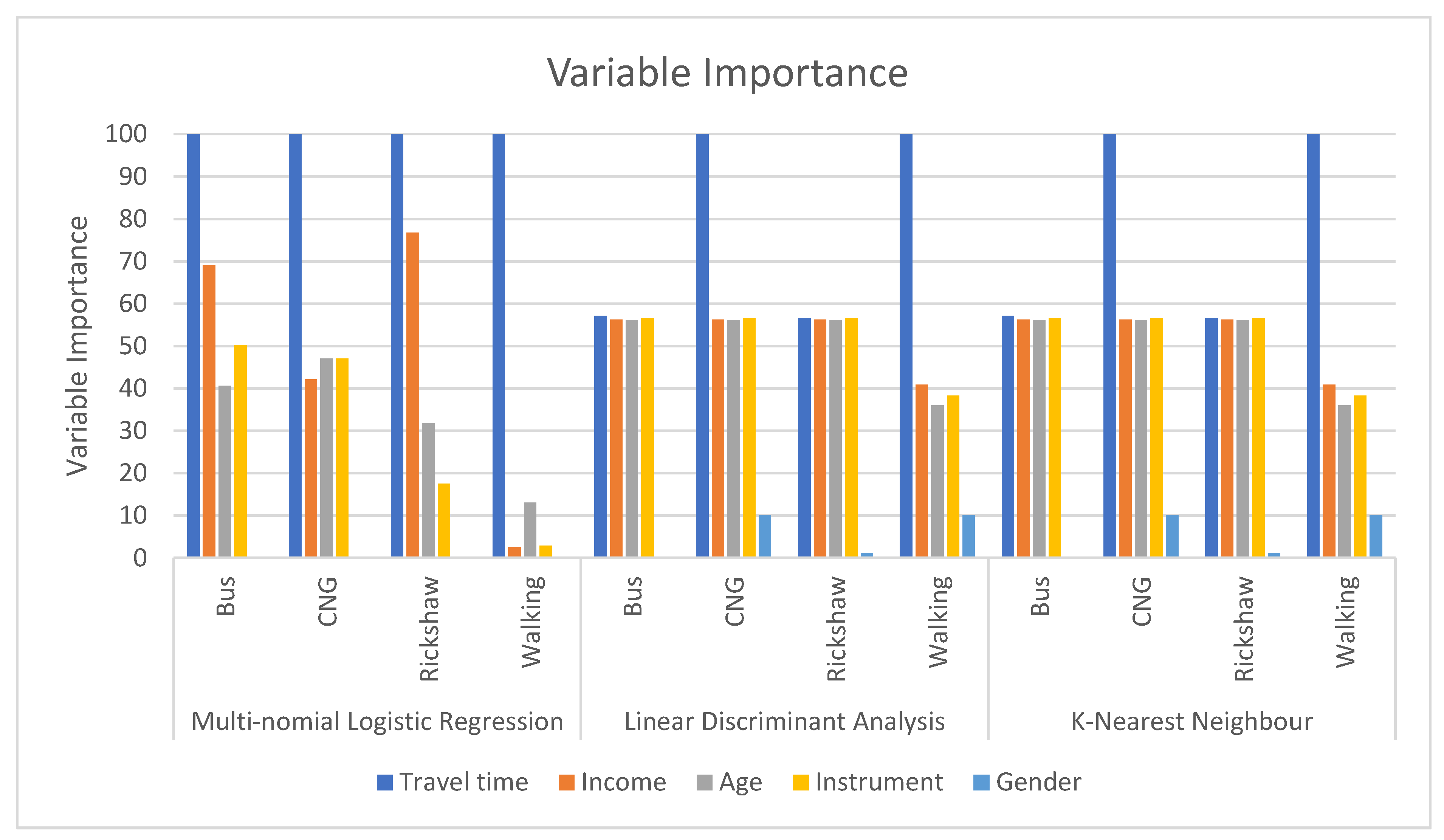
6.5. Variable Importance for Modes

Variable importance helps to understand the level of utilization of independent variables to make accurate predictions. The more a model relies on an independent variable in predicting the outcome, the higher that variable’s importance [63]. The VarImp( ) function was used to determine the variable importance of each factor in the model to make a prediction. First, age, sex, income, travel time, and supporting instrument were used in the same model to determine the variable importance. Later, each variable’s influence on the accuracy of the model was inspected by excluding each factor one at a time during development of the model. Thus, five models were developed, each excluding one of the factors, to determine the impact of that specific factor on the accuracy of the model. Figure 6 represents the variable importance for travel time, age, income, walking instrument, and sex. Travel time has been found as the most important factor in model selection for all modes for MNL. CNG and walking have the highest variable importance for LDA and KNN, while variable importance was found to be 25% for travel time for selecting rickshaw and bus as travel modes for LDA and KNN. MNL had higher variable importance for income and age in the selection of bus and rickshaw as a travel mode in comparison to KNN and LDA, and MNL had lower variable importance for income in the selection of bus and rickshaw as a travel mode in comparison to KNN and LDA. Supporting instrument had 20% or more than 20% variable importance for the selection of bus, CNG, and rickshaw for KNN and LDA, indicating that mobility impairment of MCPs plays an important role for the selection of these travel modes. In comparison to MNL, KNN and LDA had higher variable importance for supporting instruments (i.e., disability parameter) in the selection of rickshaw, bus, and walking. It can be stated that LDA and KNN found disability as a more important factor for the selection of bus, walking, and rickshaw as travel modes of MCPs. Sex was found to have no importance in the selection of travel modes from MNL. However, it was found that sex plays a (meager) role in selecting CNG, walking, and rickshaw, although the contribution is small in comparison to other factors.

Another way to explore the influence of variables in terms of prediction of mode choice within the models is to hold out individual variables from the models and assess changes in model accuracy.

Table 7. Confusion matrix KNN.

	Bus	CNG	Rickshaw	Walking
Bus	0.8125	0	0.1875	0
CNG	0.173913	0.608696	0.217391	0
Rickshaw	0.086022	0.150538	0.677419	0.086022
Walking	0.045455	0	0.045455	0.909091

reveals how the accuracy of each model changed with the exclusion of travel time, age, income, supportive instrument, and sex from the model for MNL, LDA, and KNN. An example of the calculation of accuracy is as follows:

With all the variables in the model, MNL had an accuracy of 73.38%. After running the model excluding travel time, accuracy was reduced to 57.17%.

Therefore, rate of accuracy reduction = (57.17% − 73.38%)/73.38% = −22.09%.

Accuracy of the classifiers decreased greatly with the exclusion of travel time, which is not surprising, considering its relatively higher variable importance in most instances of mode choice (as shown in Figure 6). The exclusion of supporting instruments from the models caused the second-highest change in the accuracy for all three considered classifiers. For MNL, LDA, and KNN, accuracy decreased with the exclusion of income from the model, but to a lesser extent than exclusion of travel time and supporting instrument. With the exclusion of age as a factor, accuracy decreased for LDA and KNN, but increased slightly for MNL. Travel time is a well-established factor in mode choice decision, but the contribution of supporting instrument, i.e., level of disability in second place suggests that it also has a significant impact on mode choice of MCPs (

Table 8. Change in accuracy with the exclusion of factors.

	MNL		LDA		KNN
Excluded Variable	Earlier Accuracy	New Accuracy (Change %)	Earlier Accuracy	New Accuracy (Change %)	Earlier Accuracy	New Accuracy (Change %)
Travel time	73.38%	57.17% (−22.09%)	71.43%	54.6% (−23.5%)	74.36%	55.36% (−25.5%)
Age		75.32% (+1.94%		68.91% (−3.5%)		67.04% (−9.8%)
Income		70.13% (−4.04%)		65.03% (−8.9%)		65.03% (−9.33%)
Supporting Instrument		66.23% (−9.74%)		63.95% (−10.4%)		63.9% (−12.5%)
Sex		74.03% (+0.8%)		72.34% (+1.2%)		87.14% (+17.1%)

).

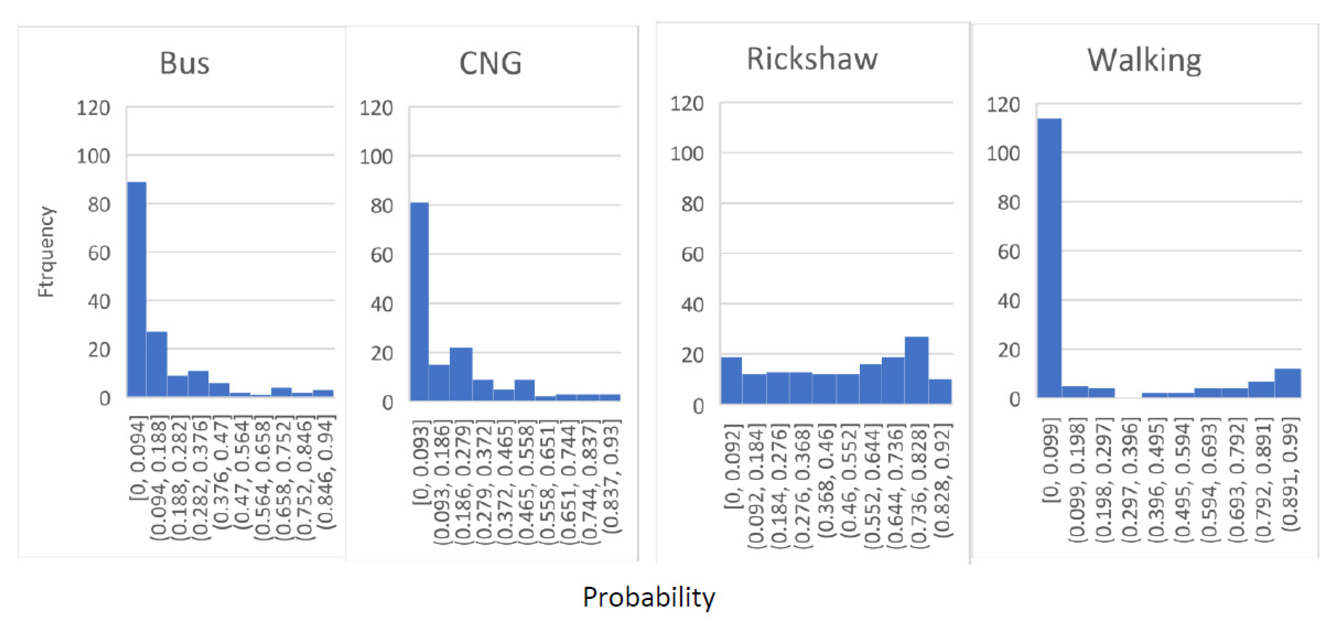
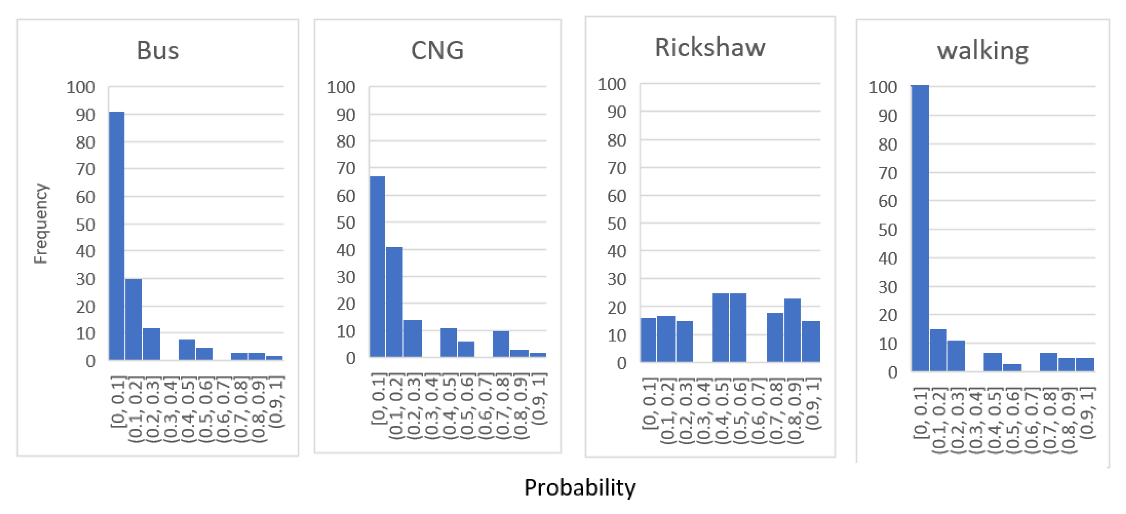
6.6. Distribution of Probability of Selecting Different Modes

Figure 7, Figure 8 and Figure 9 reveal the histogram of the cumulative distribution function (CDF) of bus, CNG, rickshaw, and walking for split ratio 0.7 for MNL, LDA, and KNN. In the figures, the X-axis represents the probability of selecting a mode of an MCP based on the developed model. The Y-axis represents how many times (i.e., frequency) a mode is found in a particular probability range by the model. CDF was developed to better understand the relationship of the probability of selecting a mode in the models and actual mode choice.

A similar pattern of probability distribution was observed for the three classification methods. Bus, CNG, and walking have positively skewed distribution and are unimodal, with a peak within the range of probability below 0.1. As the number of MCPs using bus and walking in the mode choice set is lower, bus and walking will likely have lower probability in a significant number of many instances. Although the percentage of MCPs (out of 384 samples) using CNG is relatively higher (22.91%), it is relatively smaller in comparison to that of rickshaw (47.7%), which might be the reason behind the higher number of test samples with a probability below 0.1. The frequency of selecting a rickshaw is relatively evenly distributed among different ranges of probability. Although the CDF of rickshaw has a peak around 0.73–0.82, it is not accentuated in terms of frequency.

7. Conclusions

We aimed to model the mode choice of MCPs using responses from 384 samples using ML techniques. The mode choice set for the study consisted of bus, rickshaw, CNG, and walking. In the study, we used MNL, LDA, KNN, Random Forrest, Neural Network, Naïve Bayes, and Gradient Boosting as classifiers. Accuracy, Kappa statistics, Recall, F1-score, and Precision were used as parameters to evaluate the performance of the classifiers [71]. Although it is encouraged to use ML on large datasets, the authors did not find any literature prohibiting the use of ML for the sample size 350–400. In the future, a more robust study can be conducted by including a large number of samples for developing the model with more efficient predictive capability using similar approaches to those used in this study. Similarly, apart from the variables used in this study, a large number of additional predictive variables can be included to expand the current models and explore their influences on mode choice of MCPs that have not been explored in this study. Comfort, convenience, safety, reliability, and proximity of bus and CNG stops, etc. to MCPs homes can also be included as factors in future studies. This study is focused on mode choice of MCPs for regular trips only. Research can also be conducted on the mode choice for occasional trips of MCPs using ML techniques. The methodology followed in this study can also be applied to explore mode choice of MCPs in other cities of the world.

The modal share of the MCPs demonstrates that the majority of the MCPs are using rickshaws for regular trips, followed by CNG as the second most frequent mode choice. It was found that MNL, KNN, and LDA have higher accuracy in comparison to other classifiers. Meanwhile, MNL, LDA, and RF performed better in comparison to other classifiers in respect to kappa statistics. However, along with MNL and LDA, KNN (instead of RF) was used to further explore the performance of the model, as accuracy was considered to be the more widely used parameter to assess the predictive capability of ML classifiers. Later, changes in the patterns of Precision, Recall, and F1 Score were explored for MNL, LDA, and KNN using a confusion matrix. The confusion matrix revealed that there might be overfitting by the models for bus and walking. An evenly distributed CDF function was found for rickshaw, while the CDF was found to be negatively skewed for CNG, bus, and walking.

Variable Importance functions revealed that travel time is the most influential factor in selecting mode of travel by MCPs. It is also notable that LDA and KNN found supporting instruments, i.e., level of disability as a more important factor in selecting transport mode. Interestingly, KNN and LDA showed that sex plays a role in mode selection of bus, rickshaw, and CNG, while MNL revealed sex had no role in the selection of any mode.

As supporting instrument had an almost equal level of variable importance (>55%) for rickshaw, bus, and CNG for two models: LDA and KNN, the importance of disability cannot be ignored in mode selection. Although the rickshaw is widely used by MCPs because of the convenience of door-to-door service provision, it is not without challenges, as MCPs have to contend with boarding an excessively high platform to utilize this mode of transportation. Folding ramps can be introduced in a rickshaw to make it more accessible for MCPs. Ramps should also be introduced in CNG and buses to provide universal accessibility for MCPs. The bus is considered to be one of the affordable travel modes of Dhaka city, but MCPs are travelling by expensive transportation modes like rickshaw instead. Therefore, initiatives should be undertaken to encourage the MCPs to travel by bus. There is regulation for preserving designated seats for the PWDs in buses [72]. However, this rule is rarely adhered to in practice [31]. Government should take initiatives to enforce this rule more strictly to motivate MCPs and other PWDs to travel by bus. The models also revealed that income is an important determinant of mode choice after mobility aids used by MCPs. It is likely that MCPs who have relatively lower income will prefer to pay less fare (within financial affordability). However, it is very common for rickshaw pullers and CNG drivers to charge additional fares from MCPs to exploit their lack of capacity to wait to get a vehicle with a reasonable fare. This unsavory practice increases the financial burden for MCPs with lower income. Respect towards MCPs should be created among rickshaw pullers and CNG drivers so that they do not exploit MCPs by charging additional fares because of their disability through raising social awareness and organizing training for rickshaw pullers and CNG-drivers. Government can also take the initiative to fix fares per km for the rickshaw. Although there are fixed fare structure for the CNG, this is rarely followed by CNG drivers, and greater enforcement is required [73]. Initiatives should be undertaken to rigorously monitor the maintenance of fare structure for the CNG and rickshaw. As MCPs prefer to travel by rickshaw and CNG, it is necessary for the government to take measures to keep the fares of these transport modes within the affordability of MCPs and to enforce existing laws.