Leveraging LiDAR Intensity to Evaluate Roadway Pavement Markings

Abstract

The United States has over 8.8 million lane miles nationwide, which require regular maintenance and evaluations of sign retroreflectivity, pavement markings, and other pavement information. Pavement markings convey crucial information to drivers as well as connected and autonomous vehicles for lane delineations. Current means of evaluation are by human inspection or semi-automated dedicated vehicles, which often capture one to two pavement lines at a time. Mobile LiDAR is also frequently used by agencies to map signs and infrastructure as well as assess pavement conditions and drainage profiles. This paper presents a case study where over 70 miles of US-52 and US-41 in Indiana were assessed, utilizing both a mobile retroreflectometer and a LiDAR mobile mapping system. Comparing the intensity data from LiDAR data and the retroreflective readings, there was a linear correlation for right edge pavement markings with an R² of 0.87 and for the center skip line a linear correlation with an R² of 0.63. The p-values were 0.000 and 0.000, respectively. Although there are no published standards for using LiDAR to evaluate pavement marking retroreflectivity, these results suggest that mobile LiDAR is a viable tool for network level monitoring of retroreflectivity.

1. Motivation

The United States has over 8.8 million lane miles nationwide, which all require regular maintenance and evaluation of sign retroreflectivity, pavement markings, and other pavement information. Pavement markings convey crucial information to drivers as well as connected and autonomous vehicles for lane delineations. Current evaluation strategies are conducted by human inspection or semi-automated dedicated vehicles which often capture one to two pavement lines at a time. Pavement markings deteriorate overtime due to tire wear, weather, and snowplow wear, making the markings difficult-to-detect for human and autonomous vehicles.

Difficult-to-detect pavement markings can increase driver workload and cause driver confusion, particularly during more challenging driving conditions such as nighttime and/or inclement weather. Determining locations where vehicles cannot detect pavement markings is especially important in the new frontier of connected and autonomous vehicles. A study conducted by the National Cooperative Highway Research Program (NCHRP) found that approximately 30% of state agencies conduct annual pavement marking evaluations, and the remaining 70% do so on a bi-annual or more sporadic basis [1].

Common types of pavement markings utilized by agencies include multi-component, paint, preformed tape, and thermoplastic. The installed pavement marking is based on several unique factors, but often depends on an agency’s budget, maintenance procedures, and labor force [2]. Pavement marking evaluation frequency varies by agency, but most agencies use the American Society for Testing and Materials (ASTM) Standard D7585 and ASTM Standard E1710 depending on the instrument being used to evaluate the pavement marking [3,4]. Compared to the handheld unit, the mobile unit enables agencies to evaluate pavement markings efficiently. A limitation of this method is that the unit only detects retroreflectivity on one pavement marking at a time. Hence, the unit needs to make six passes to evaluate a four-lane divided highway.

Mobile Light Detection and Ranging (LiDAR) has the ability to evaluate multiple lanes with one sensor, with a single pass (i.e., the system only needs two passes for a four-lane divided highway). This paper evaluates using LiDAR sensors to provide scalable methods that will allow agencies to systematically evaluate their road markings and routinely program their maintenance activities.

2. Literature Review

Various methods are used to evaluate pavement markings including LiDAR-based systems, retroreflective readings, and new approaches introduce the utilization of advanced driver assistance systems [5]. Retroreflective readings are the most common accepted practice and several studies [6,7,8,9] have been completed that report a statistical correlation between lane marking retroreflectivity and the number of crashes. Retroreflectivity evaluation relies on handheld or vehicle-mounted devices. Handheld devices are typically used for job site inspection, and mobile devices are typically used for network screening. Using mobile retroreflectometers mounted to the side of a vehicle, which is safer and faster than manual evaluation, is still limited to only adjacent lane markings (one lane) evaluated at a time.

Recently, LiDAR-based mobile mapping systems (MMS) have been widely adopted by the Departments of Transportation (DOT). Approximately 50% of the DOTs indicated that they have utilized LiDAR-based MMS for applications related to engineering survey, mapping, and digital terrain modeling (DTM) [10]. This trend is motivated by the fact that LiDAR scanners can deliver 360-degree surround perception under different lighting and weather conditions. Even if the intensity readings are affected by hazy or rainy conditions, a mathematical model (as a function of LiDAR maximum range and rain rate) for the degradation of LiDAR intensity values can be used to minimize the impact as suggested by Filgueira et al. [11] and Goodin et al. [12].

A search of the literature describing LiDAR evaluation of retro reflectivity yielded only one study comparing LiDAR intensity and retroreflective measurements. Che et al. [13] converted intensity values into retroreflectivity readings through an empirical model, which is determined based on the operation principles of a handheld retroreflectometer. According to their comparison, the root mean squared error (RMSE) between the retroreflectivity estimated from mobile LiDAR and the handheld retroreflectometer readings is approximately 37.4 mcd∙m⁻²∙lx⁻¹ (the handheld retroreflectometer provides readings within 0–2000 mcd∙m⁻²∙lx⁻¹). No literature was identified that reported on the relationship between LiDAR intensity values and the mobile retroreflectivity readings. Identifying relationships between LiDAR intensity and retro reflectivity provides additional use cases for MMS because the same LiDAR data can be utilized for various transportation applications, such as lane marking extraction [14,15,16,17,18] and road feature detection [19,20,21].

Lane markings exhibit higher reflectiveness than nearby road surfaces since retroreflective glass beads are incorporated into the paint. This contrast will be pronounced in LiDAR data, which encompasses both the reflectivity and position information in the form of point clouds with intensity values. LiDAR point clouds have been utilized to extract lane markings through intensity-based approaches. The extraction approaches can be divided into two main categories: (a) LiDAR intensity image-driven and (b) LiDAR point cloud-driven. For intensity image-based approaches, Chen et al. [14] detected lane markings from the rasterized intensity images. They identified candidate lane markings from road surface point clouds using adaptive thresholding, where thresholds were invariant to intensity values and converted the candidate points to intensity images. Lane markings were then extracted from the images through Hough transform [22], followed by a refinement based on the trajectory data. Guan et al. [15] generated intensity images by the modified inverse distance weighting (IDW) interpolation to identify lane markings. Lane marking pixels were detected from the images through a multi-scale tensor voting (MSTV) algorithm [23]. The results were further grouped by a region-growing approach for each lane marking. However, in all such intensity image-based approaches, the original accuracy and intensity information would be lost due to the point cloud rasterization. Therefore, several researchers began to extract lane markings directly from point clouds. Vosselman et al. [16] presented range-dependent thresholding to identify lane markings from point clouds. Lane marking points were detected by an intensity threshold, which was determined based on the range. After that, the detected marker points were grouped together using connected component analysis [24]. Yu et al. [17] also extracted lane markings directly from point clouds. They partitioned the road surface point cloud into several segments across the driving direction. For each segment, lane marking points were identified using an intensity-based threshold determined by the range and incident angle of the segment. A spatial density filter was finally applied to the identified points for false positive removal. Cheng et al. [18] proposed an intensity thresholding strategy using unsupervised intensity normalization [25] and a deep learning strategy using automatically-labeled training data for lane marking extraction. For the intensity thresholding strategy, lane markings were directly extracted from the normalized point clouds. These extracted lane markings were then utilized to generate training samples automatically to train a U-net model for the deep learning approach. Moreover, based on the automated labeling procedure, Patel et al. [26] presented a transfer learning approach for fine-tuning a model trained by earlier data using only a few training samples from new datasets.

Additionally, most road characteristics, such as lane width, potholes, and roadside ditches, can be automatically identified from LiDAR data. For instance, Ravi et al. [19] proposed a fully automated framework based on LiDAR data. After lane marking extraction from point clouds, the detected markings were classified into left and right groups according to the driving direction. Thereafter, the centerline points of each group were generated and utilized to estimate lane width. Ravi et al. [20] conducted pavement anomaly detection (including cracking, potholes, and debris) using point clouds. First, points that exhibit some form of discontinuity within each scan line were detected according to the geometric information. Based on these points, the cracking, potholes, or debris were identified through local neighborhood analysis. Furthermore, Lin et al. [21] explored the possibility of using LiDAR data collected by various MMSs (including an unmanned aerial vehicle, an unmanned ground vehicle, and wheel-based systems) for mapping roadside ditches. They indicated that roadside ditch mapping using wheel-based systems is more efficient and can cover a large area that is impractical with an unmanned aerial or ground vehicle.

In addition, LiDAR data, which precisely provides 3D coordinates and intensity information, could reduce or overcome the difficulties of traditional photogrammetric techniques, such as capturing terrain topography [27,28,29] and true orthoimage generation [30,31]. Stal et al. [27] utilized stereoscopic aerial images and LiDAR point clouds to generate digital surface models (DSM) over an urban area for change detection. Balsa-Barreiro and Fritsch [28] proposed an approach based on laser scanning and photogrammetric techniques for surveying historical cities. Owda et al. [29] reconstructed 3D photorealistic models through laser scanning and photogrammetric datasets. They found that the usage of combined data has optimized the processing. For true orthoimage generation, Shin and Lee [30] presented a generative adversarial network (GAN)-based approach for true orthoimage generation. They utilized LiDAR intensity readings to improve the performance of the GAN model. Recently, Mok and Kim [31] proposed a GAN-based approach for generating simulated intensity values of LiDAR data. Real LiDAR data from MMS were fed inputs to train a GAN model for intensity simulation. They believe that, in the future, a GAN-based model can be used to simulate LiDAR intensity for MMS under various environments. Consequently, the relationship between intensity values and mobile retroreflectivity readings can be the basis of these intensity-based studies.

3. Study Objectives

The objective of this study was to determine if there is statistical correlation between retroreflective measurements and LiDAR intensity measurements so that an agency could use LiDAR data to screen their network for sections that have degraded in retroreflectivity. Additionally, this study observed potential methods that could be used by agencies to assess several components of infrastructure with a single sensor. Specifically, this study collected data for 70 miles of white center skip lines and right edge lines and compared:

• ASTM E1710 Retroreflectivity vs. LiDAR Intensity
• IR Retroreflectivity vs. LiDAR Intensity

4. Equipment, Datasets, and Methods

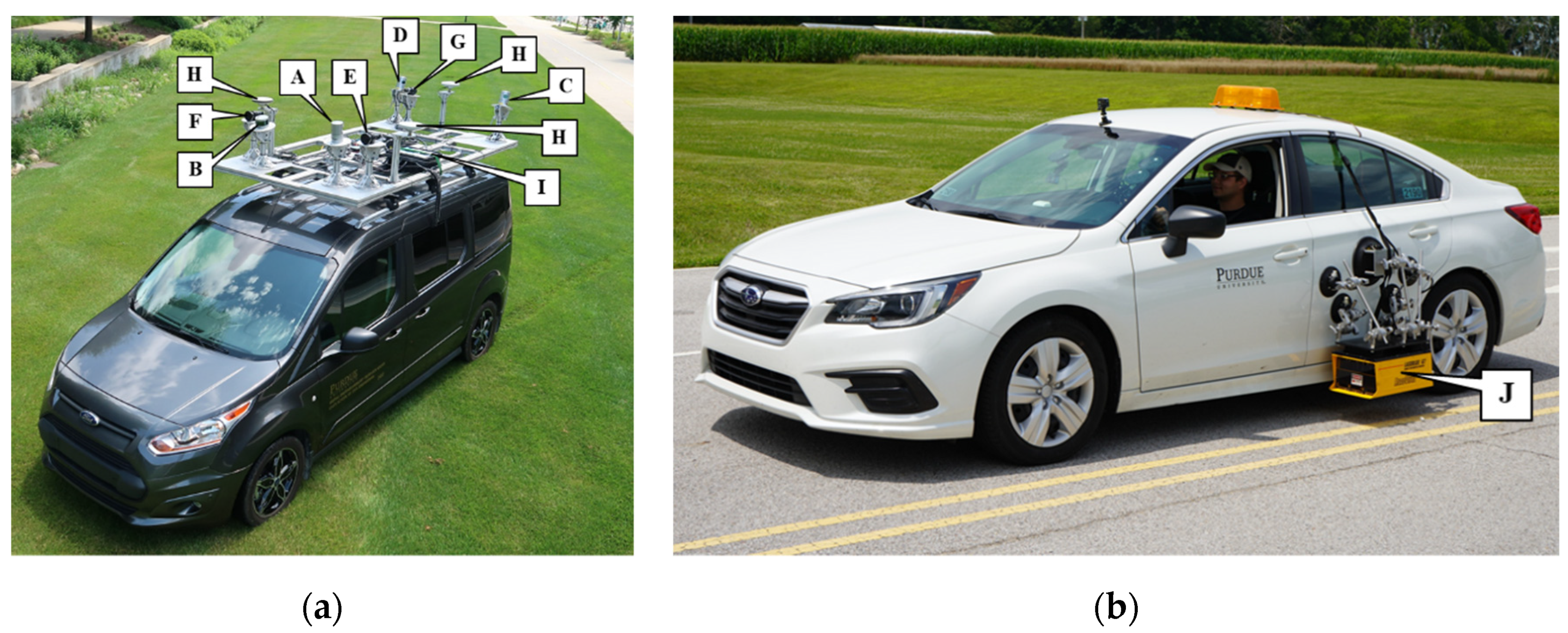
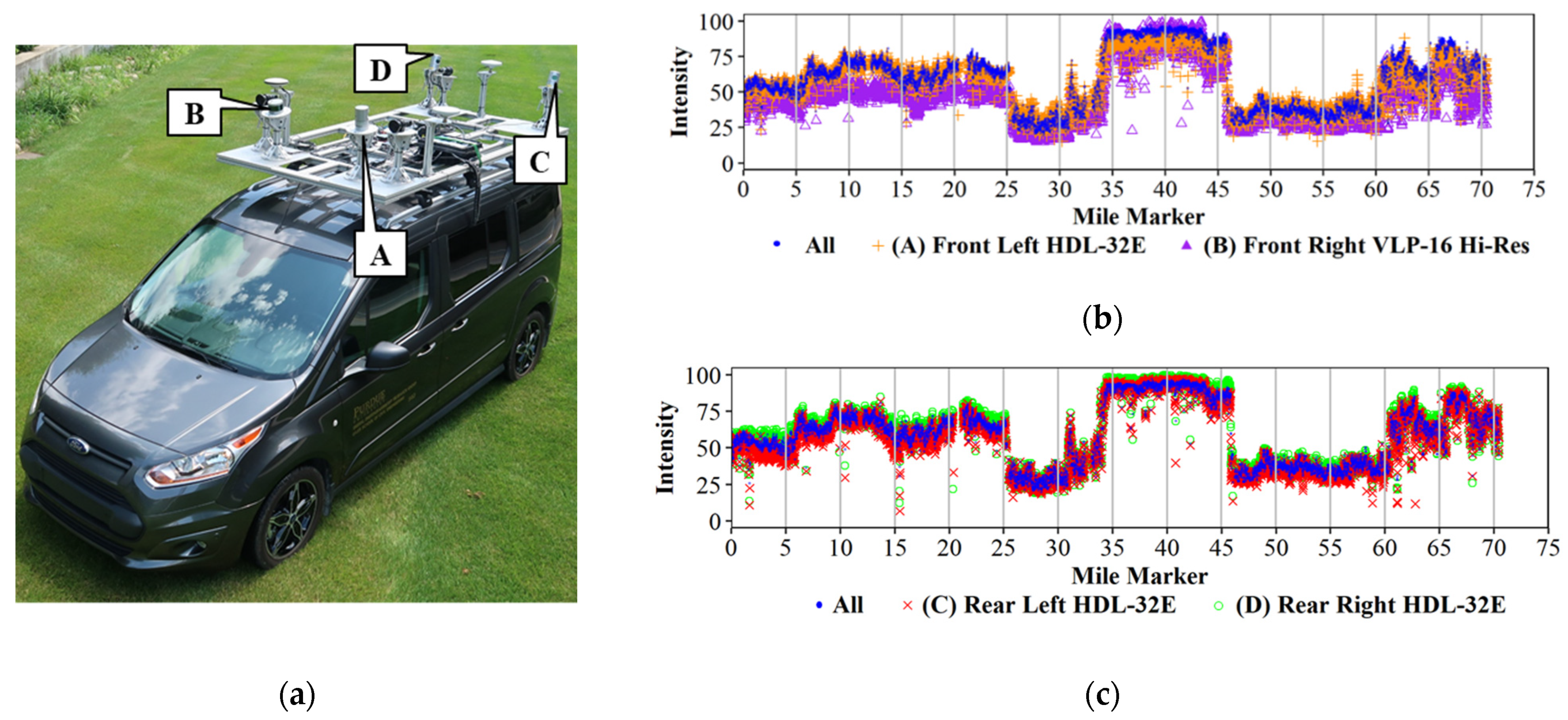
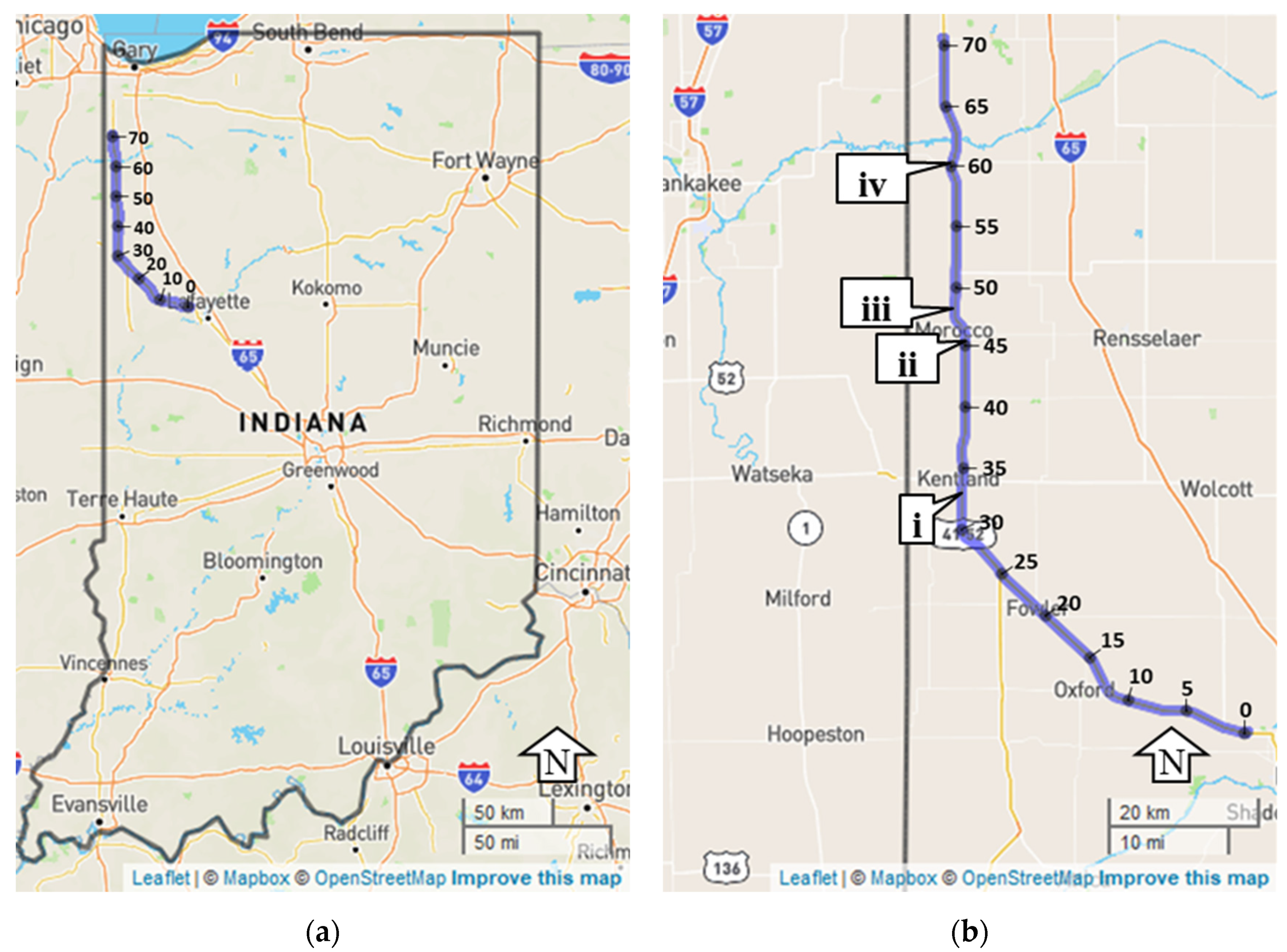
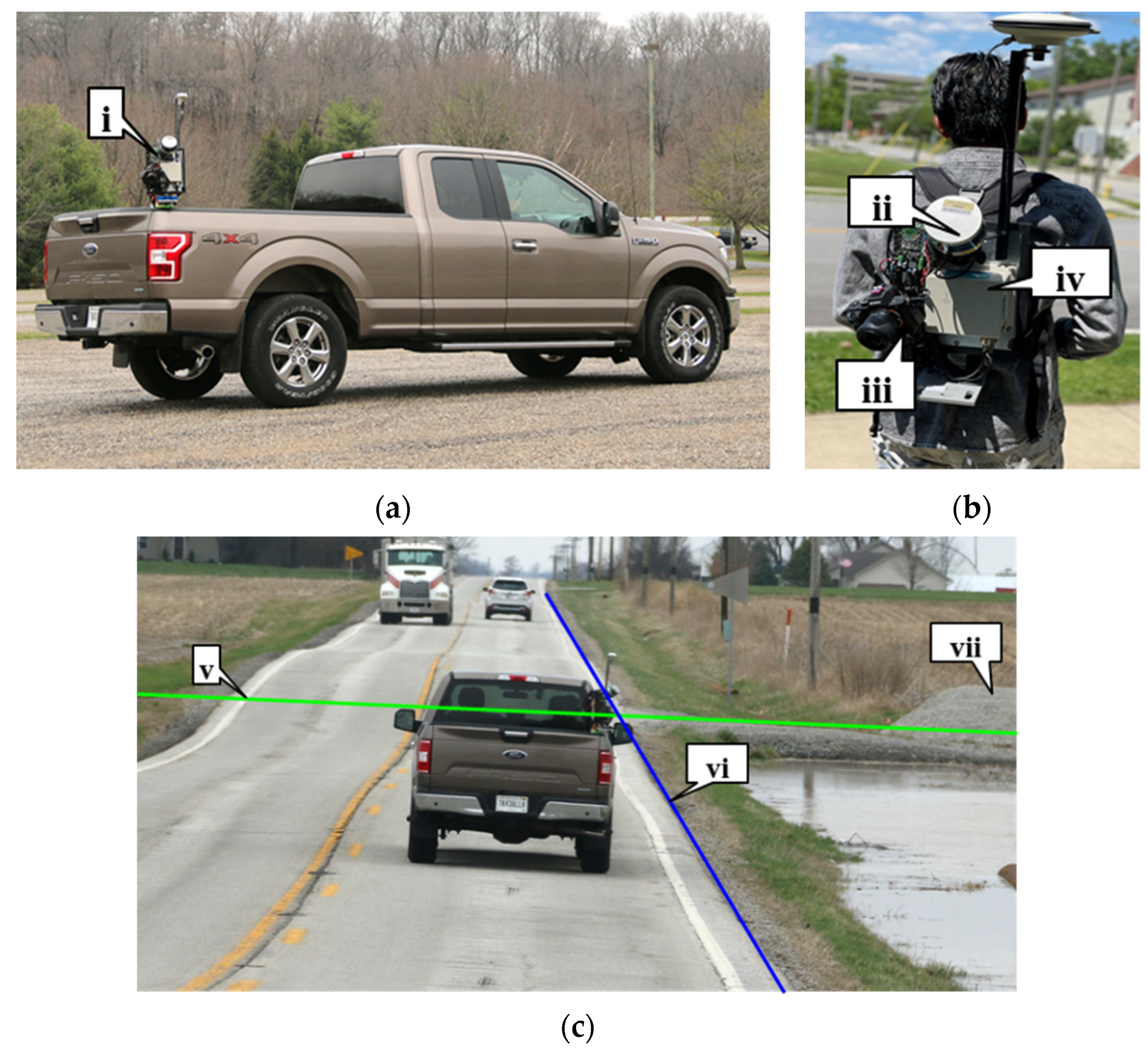
4.1. Study Route and Equipment

The study was conducted along 70-miles of US-41 and US-52 in rural Indiana (Figure 1a,b). The route runs from West Lafayette, Indiana to Lowell, Indiana. Two vehicles (Figure 1c) traversed this route. The lead vehicle (Purdue mobile mapping system) was a mobile mapping unit equipped with LiDAR (Figure 2a) and the trailing vehicle was a passenger car equipped with a Road Vista Laserlux G7 (LLG7) (Figure 2b). Both lead and trailing vehicles drove at an average speed of 50 mph. Callouts i through iv are example cases that are discussed in Section 4.4 of the report.

The Purdue Mobile Mapping System, seen in Figure 2a, has four LiDAR units: three are Velodyne HDL-32Es seen in the front left (callout A), rear left (callout C), rear right (callout D), and one VLP-16 unit on the front right (callout B). The vehicle is also equipped with three RGB cameras in the front left (callout E), front right (callout F), and a rear facing camera (callout G). The remote sensing units and images are georeferenced with a global navigation satellite system/inertial navigation system (GNSS/INS) unit (callout I) and the antenna for the unit being depicted in callout H. The Purdue fleet vehicle, seen in Figure 2b, was equipped with an LLG7 (callout J) and made one pass to capture the right edge marking and then repositioned the sensor and mounted the unit on the driver side and made an additional pass to capture the center line skip marking.

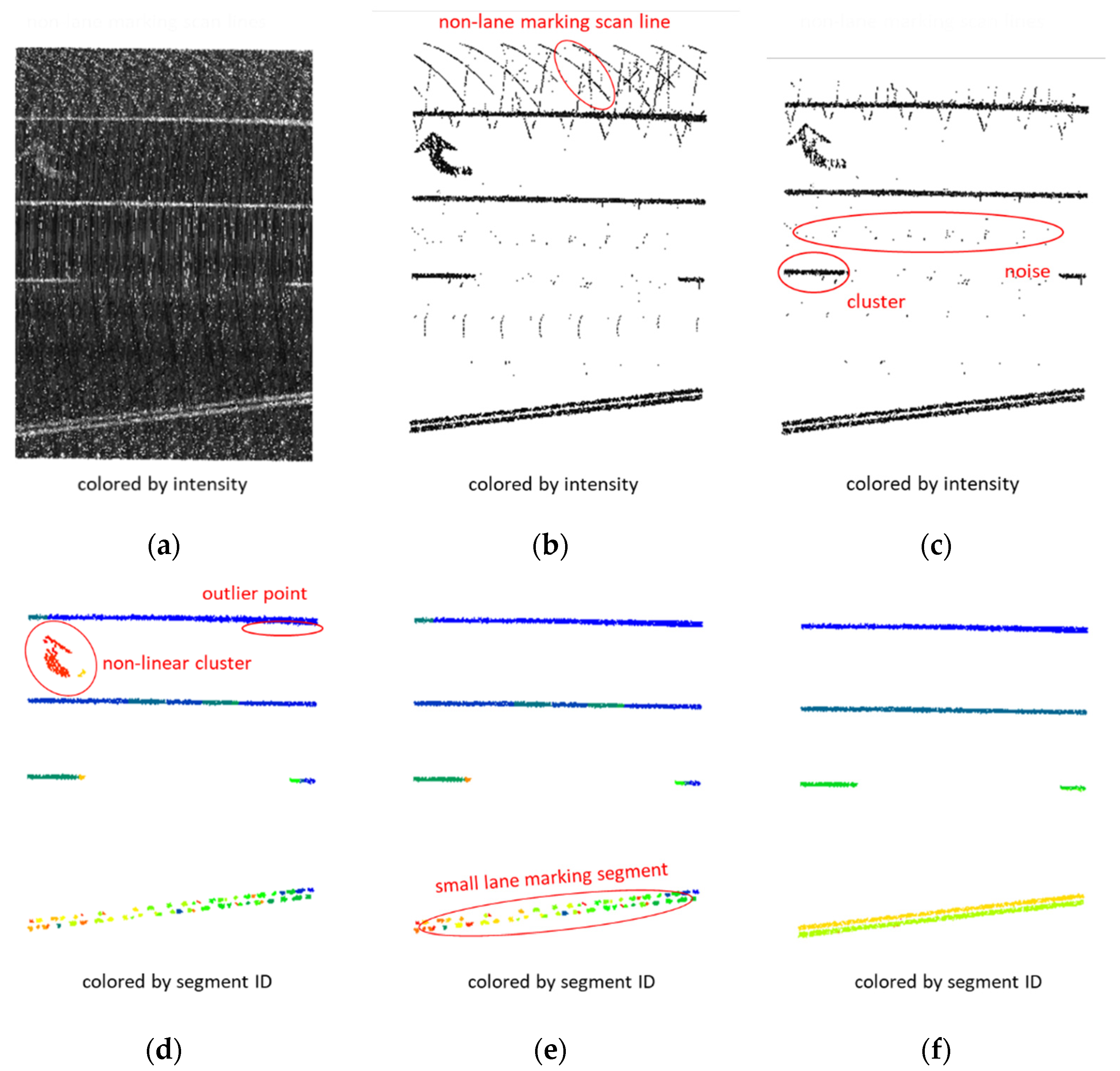
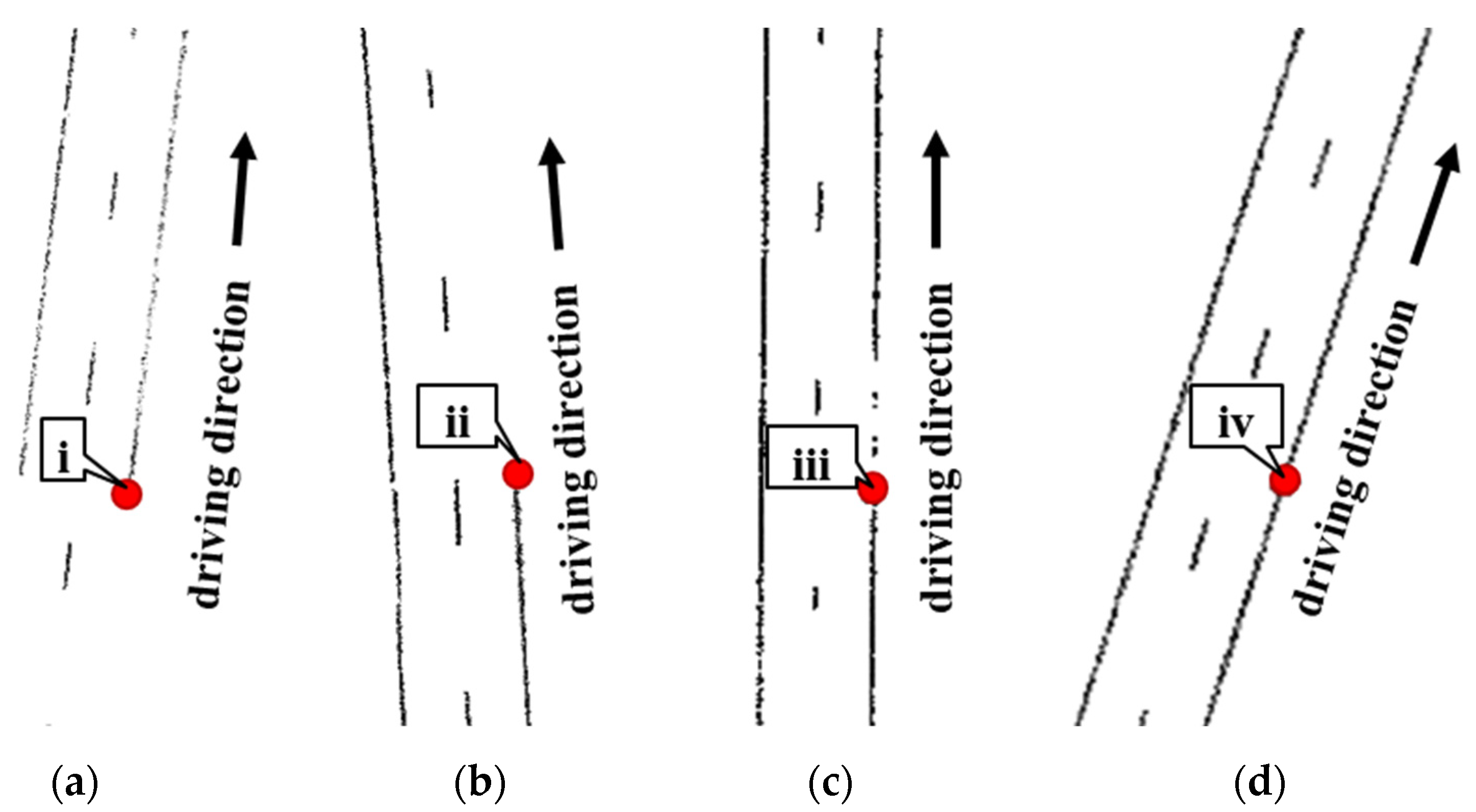
4.2. Lane Marking Extraction from LiDAR Point Clouds

Through a system calibration procedure, mounting parameters between LiDAR units and a GNSS/Inertial Measurement Unit (IMU) navigation system were estimated, facilitating the reconstruction of georeferenced, well-registered point clouds from the LiDAR scanners [32]. The reconstructed point clouds are divided into 12.8 m (along driving direction) by 16m (across driving direction) blocks. Road surface points are then extracted from each block through a height buffer-based strategy [19]. Finally, lane markings are identified through the following steps: (i) 5th percentile intensity thresholding, (ii) scan line-based outlier removal, (iii) density-based spatial clustering [33], (iv) geometry-based outlier removal, and (v) local and global refinement. For a given road surface block, as displayed in Figure 3a, hypothesized lane markings are extracted by step (i), as shown in Figure 3b. Then, step (ii) is applied to the hypothesized lane markings. This removal approach assumes that scan lines within a lane marking must not exceed a certain length since a lane marking has a finite width. After step (ii), as shown in Figure 3c, the remaining lane marking points need to be grouped into isolated lane marking segments. To achieve this, density-based spatial clustering is adopted. This clustering algorithm is particularly useful in the grouping since hypothesized lane markings are still subject to low-point-density noise, as depicted in Figure 3c. Another advantage of adopting this algorithm is that lane marking points can be grouped into isolated segments, as shown in Figure 3d, which helps the subsequent analysis. Next, a geometry-based strategy is conducted to remove non-linear segments as well as outlier points within a linear segment, as shown in Figure 3e. Finally, in order to connect isolated small segments, two refinement strategies are conducted. First, local refinement aims to connect small marker segments within each block as well as identify undetected lane marking points between small segments. Then, global refinement, which focuses on combining the same lane marking segments located in successive blocks, is applied to all extracted lane markings. The final extraction is shown in Figure 3f.

4.3. Retroreflective Data

The retroreflectometer provided an accumulated average retroreflective reading every ten feet and has an internal Global Positioning System (GPS) to provide the geolocation of the measurement. To evaluate and compare the data, the two geospatial datasets were aggregated, averaged, and linearized to the nearest 0.01 mile along the study route.

4.4. Linear Referenced Retroreflectivity and LiDAR Intensity

To evaluate the pavement markings, the linearized data was plotted along the route. Figure 4a shows the infrared retroreflective measurements along the vertical axis and the spatial mile markers along the horizontal axis, Figure 4b follows a similar structure and shows the standard retroreflective measurements on the vertical axis, and Figure 4c shows the LiDAR intensity on the vertical axis. The shown values are the readings observed on the center skip line. The vertical red line on Figure 4 is the location where US-52 merges with US-41 northbound. A similar comparison can be seen in Figure 5 for the right edge marking. Overall, the trend between infrared and standard retroreflective readings is comparable to those of LiDAR intensity at the same point.

5. Results and Discussion

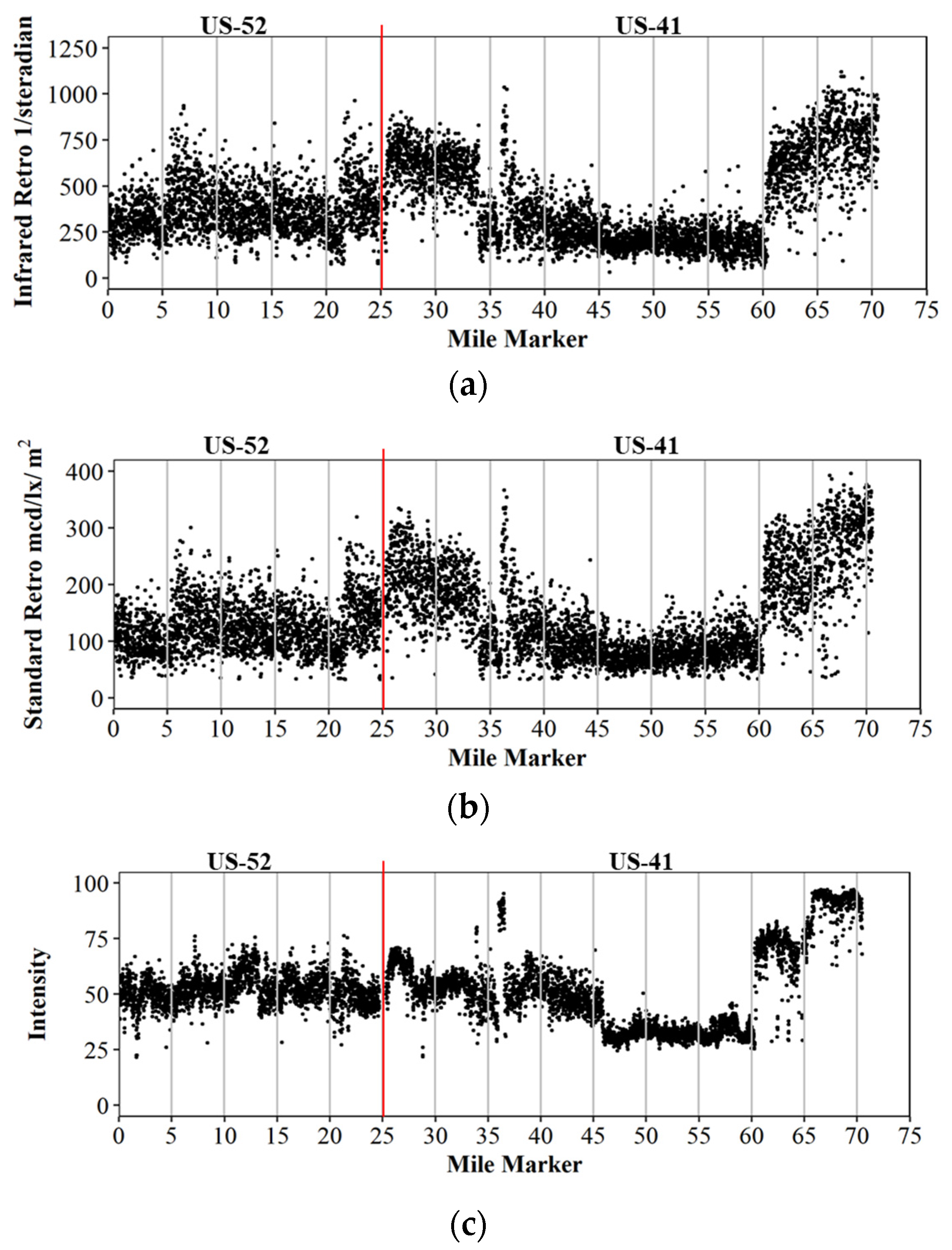
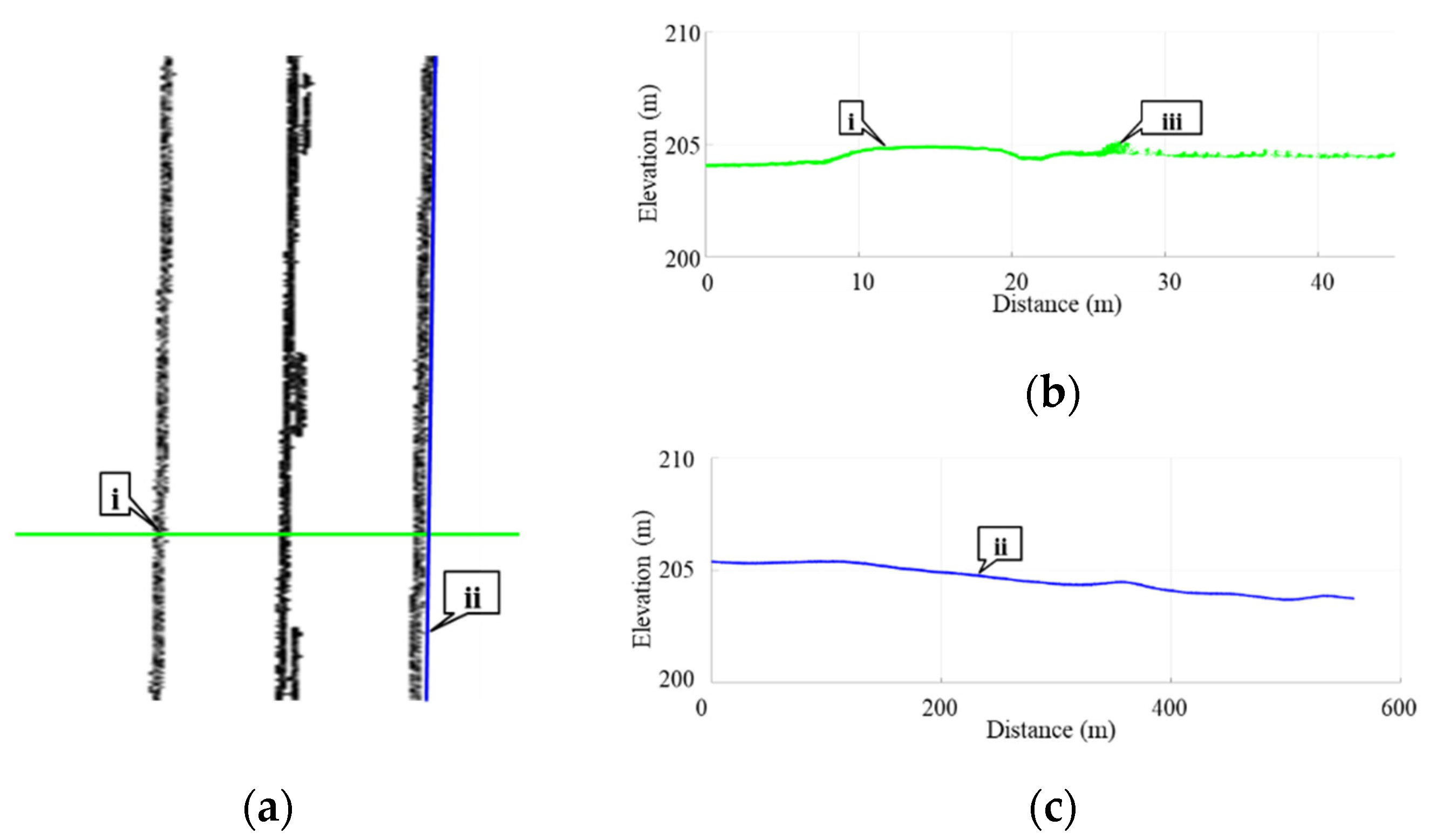
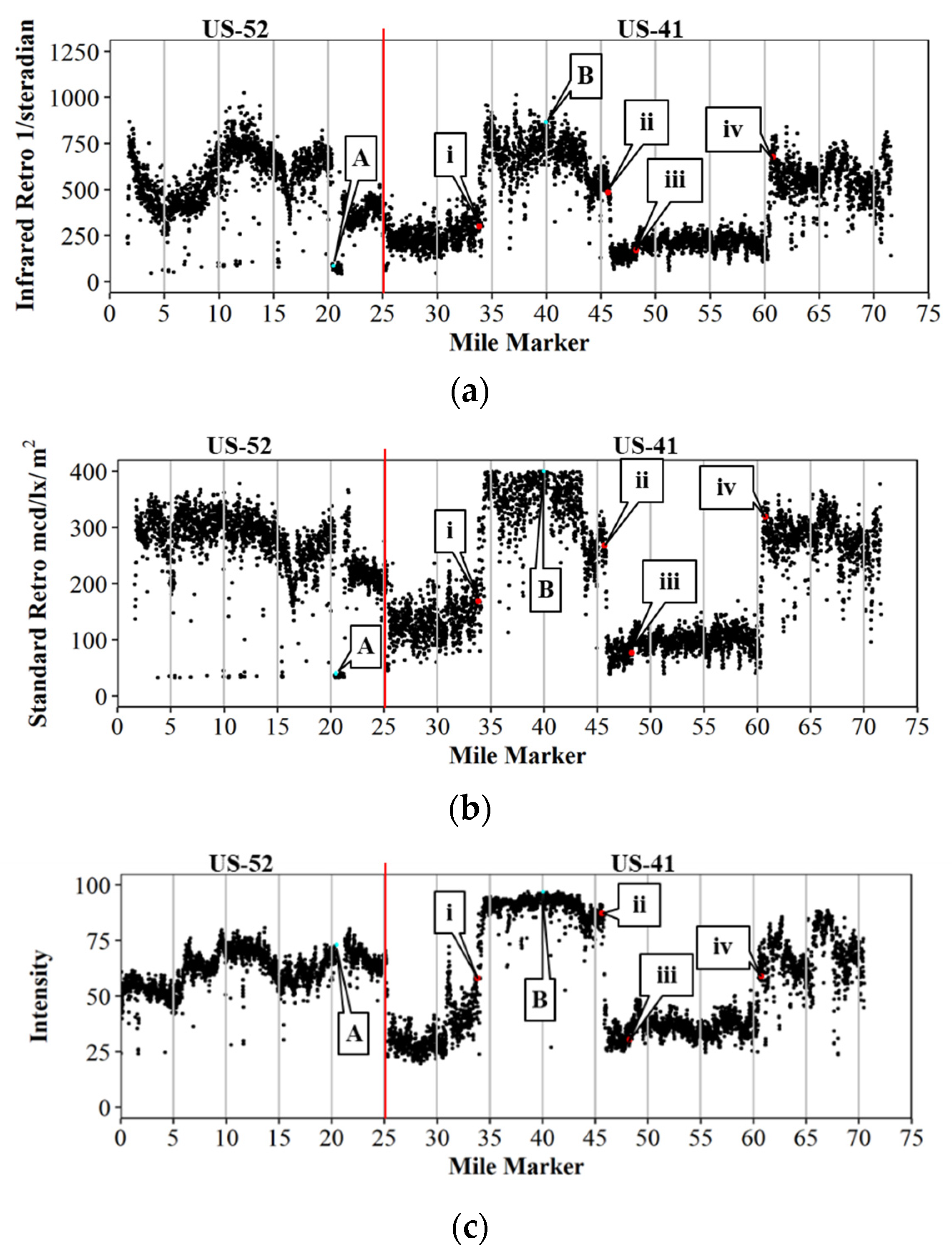
5.1. Qualitative Comparison

A qualitative comparison was conducted to validate the lower and higher retroreflective and intensity values. Figure 6 shows the georeferenced images for the callout locations in Figure 5. Callout i in Figure 6a is the same location as the red point in callout i on Figure 5. Figure 6a shows the lack of pavement markings on the left edge and right edge of the driving surface, callout i depicts the point when the pavement markings resume. Figure 6b shows a transition location going from high retroreflective and intensity values to lower values and callout ii depicts the transition point. Figure 6c is an example of a location with low retroreflective and intensity values, callout iii shows the deteriorating pavement marking on the right edge line. Figure 6d shows the location where there are high retroreflective and intensity values.

The corresponding LiDAR intensity profiles for each representative photo can be seen in Figure 7. Callouts i, ii, iii, and iv in Figure 7 are the same locations depicted in Figure 5 and Figure 6, respectively. The LiDAR intensity profiles provide greater context to the intersection gap of pavement markings viewed in Figure 7a, lack of pavement marking presence seen in Figure 7b, deteriorated pavement marking observed in Figure 7c, and easily visible pavement marking presence viewed in Figure 7d.

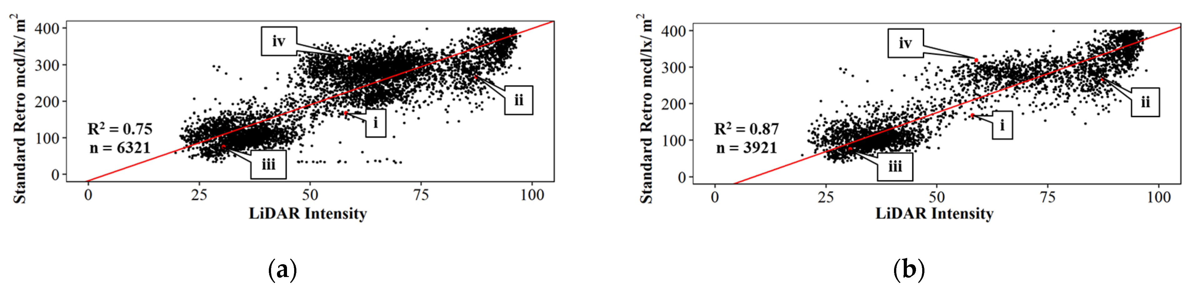
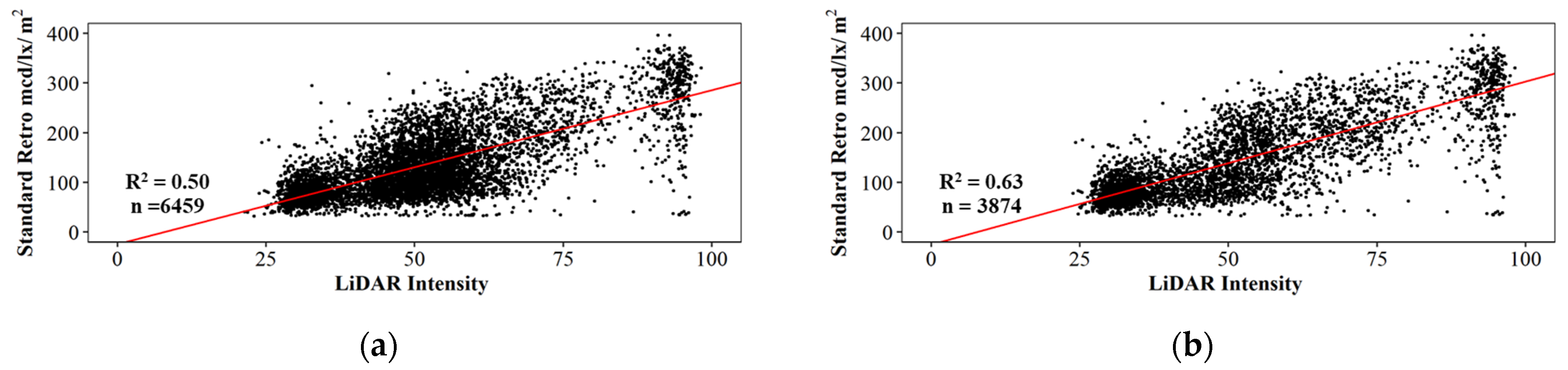
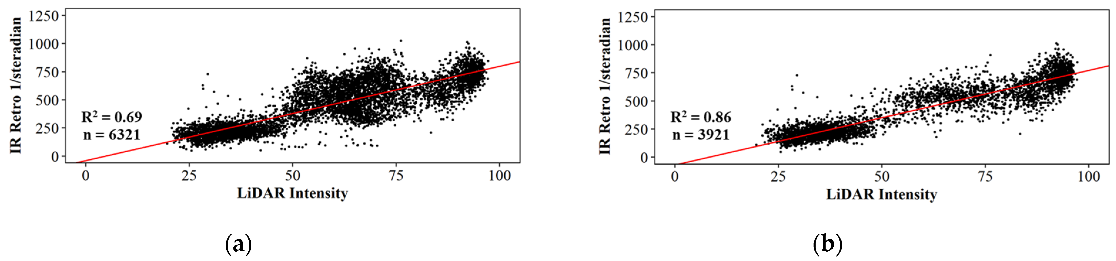
5.2. Correlation between Retrorefelctity and LiDAR Intensity

The extracted lane marking point clouds and corresponding retroreflective reading points within regions where lane markings are absent (intersection) and present (high-intensity or high-retroreflective values) are displayed in Figure 8a,b, respectively. Locations A and B in Figure 8 are the same locations in Figure 5. For areas where lane markings are absent, as can be seen in Figure 8a,c, the lane marking is undetected by LiDAR scanners and both infrared and standard retroreflective values are low. Conversely, within a complete lane marking region, the lane markings are identified clearly, and the infrared and standard retroreflective readings are high, as shown in Figure 8b,d. One should note that the retroreflective reading points might not be aligned with lane marking point clouds, as the points in Figure 8b, due to varying accuracy of the geo-location systems for the different units.

To provide a statistical evaluation of this relationship, retroreflective and LiDAR intensity values were aggregated for each 0.01-mile and plotted in a scatter plot. The scatter plot in Figure 9 shows retroreflectivity vs. LiDAR intensities for the center skip line along the 70-mile study route. A linear trend-line is then plotted over the data points that had an R² of 0.50. In addition, a Pearson test was performed with a null hypothesis of no linear correlation against the alternative hypothesis that there is a correlation. The Pearson’s correlation coefficient was calculated to be 0.72. The corresponding p-value of 0.000 suggests there is statistical evidence to reject the null hypothesis. The road surface of US-52 contained a high level of crack sealing along and on the pavement marking, causing noise in the dataset. Removing the data points along US-52 and observing the linear regression on US-41, the R² increased to 0.63 for the center skip lines and Pearson’s correlation coefficient increased to 0.79. Additionally, the calculated p-value of 0.000 rejects the null hypothesis. Figure 10a depicts the road surface on US-52 and the crack sealing applied on the road surface. Callout i shows the crack sealant partially covering the pavement marking. Figure 10b shows the US-41 pavement surface and the lack of crack sealing activities. Callout ii shows the unobstructed center skip line. The analysis was also completed for the right edge line, which can be observed in Figure 11. Figure 11a shows the linear trend between LiDAR intensity and standard retroreflectivity with an R² of 0.75, but similar to the center skip line, the crack sealant caused noise in the data and removing the datapoints along US-52 improved the linear relationship and the R² increased to 0.87, as shown in Figure 11b. A Pearson test was performed for both cases and p-values for each analysis of 0.000 suggest there is statistical significance to reject the null hypothesis of no linear correlation.

Additionally, a linear regression was completed for infrared retroreflectivity and LiDAR intensity for the center skip line and right edge line. The trends observed were similar to the standard retroreflectivity with the combined center skip line having an R² of 0.54 (Figure 12a) and focusing on the linear relationship for US-41 having an increased R² of 0.66 (Figure 12b). For the whole dataset on the right edge line, the linear trendline had an R² of 0.69 (Figure 13a) and after removing the noisy data points on US-52, the R² increased to 0.86 (Figure 13b). A Pearson test was performed for all four cases and p-values for each analysis of 0.000 suggests there is statistical significance to reject the null hypothesis of no linear correlation.

The R² for the center skip line and the right edge line establishes that there is a linear relationship between retroreflective values and LiDAR intensities. This relationship accomplishes the first objective of the study; to enable deployment and use for agencies. The secondary objective of how many LiDAR sensors would be necessary and the position on the vehicle was evaluated to optimize agency use and deployment.

Figure 14b shows the LiDAR intensities from the well-registered/georeferenced combined point cloud from all sensors compared to the individual intensity received from the individual sensor on the front left, seen in callout A on Figure 14a and front right LiDAR, seen in callout B on Figure 14a. Similarly, the combined intensities were compared to the rear sensors in Figure 14c. The rear left sensor can be seen in callout C on Figure 14a and the rear right sensor can be seen in callout D on Figure 14a.

To fully analyze if there was an impact of LiDAR sensor location on the recorded intensity, linear regression was performed to determine if there was a lateral or longitudinal difference. Figure 15a shows a scatter plot of the front left (FL) against the rear left (RL) intensities for the right edge line along the 70-mile study route. A linear trendline is plotted over the data points, which returned an R² of 0.95. A similar plot can be seen in Figure 15b that shows the rear right (RR) against the front right (FR), having an R² of 0.9. Figure 15c is a plot of the front left against the front right with an R² of 0.87 and Figure 15d is a plot of the rear left against the rear right with an R² of 0.98. Overall, the R² values were quite high. The two relationships with the lowest R² had a different sensor type with fewer laser beams, which is likely the cause of the difference. A Pearson test was performed for all four cases and p-values for each analysis of 0.000 suggest there is statistical significance to reject the null hypothesis of no linear correlation. Overall, this relationship indicates there is no statistical difference between the location of the LiDAR sensor and the intensities for pavement marking analysis indicating LiDAR evaluation can be performed with a single calibrated LiDAR sensor with the accompanying equipment. A summary of R² values, Pearson correlation coefficients, and p-values for each comparison can be seen in

Table 1. Summary of statistical analysis.

Study Location and Comparisons	R2	Pearson Correlation Coefficient	p-Value
US-52 & US-41 Standard Retroreflectivity vs. LiDAR Intensity Center Skip Line	0.50	0.72	0.000
US-41 Standard Retroreflectivity vs. LiDAR Intensity Center Skip Line	0.63	0.80	0.000
US-52 & US-41 Standard Retroreflectivity vs. LiDAR Intensity Right Edge Line	0.75	0.86	0.000
US-41 Standard Retroreflectivity vs. LiDAR Intensity Right Edge Line	0.87	0.93	0.000
US-52 & US-41 Infrared Retroreflectivity vs. LiDAR Intensity Center Skip Line	0.54	0.73	0.000
US-41 Infrared Retroreflectivity vs. LiDAR Intensity Center Skip Line	0.66	0.81	0.000
US-52 & US-41 Infrared Retroreflectivity vs. LiDAR Intensity Right Edge Line	0.69	0.83	0.000
US-41 Infrared Retroreflectivity vs. LiDAR Intensity Right Edge Line	0.86	0.93	0.000
US-52 & US-41 LiDAR Intensity Front Left vs. Rear Left	0.95	0.98	0.000
US-52 & US-41 LiDAR Intensity Rear Right vs. Front Right	0.90	0.95	0.000
US-52 & US-41 LiDAR Intensity Front Left vs. Front Right	0.87	0.94	0.000
US-52 & US-41 LiDAR Intensity Rear Left vs. Rear Right	0.98	0.99	0.000

.

6. Conclusions and Recommendations for Future Research

6.1. Additional Data Collection Opportunities with LiDAR

It is not uncommon that agencies drive their roads multiple times a year with different data collection systems, often with different spatial accuracy. Mobile LiDAR mapping of multiple infrastructure elements (grade, profiles, bridge clearance, sign height, sign placement, drainage) in a single pass is highly desirable from both a manpower and a data consistency perspective.

The mobile mapping system shown in Figure 2a had four sensors so we could assess alternative sensor placement. However, by looking at Figure 14 and Figure 15, it is clear that a single sensor can be used to evaluate the retroreflectivity of multiple lanes in one pass. To illustrate the synergies between assessing pavement marking conditions and other mobile mapping systems, a single sensor mobile mapping system is shown in Figure 16a. The results in this study support the use of a single LiDAR scanner mounted on a vehicle seen in Figure 16a callout i. The self-contained unit (Figure 16b) includes a single LiDAR Unit (callout ii), a camera (callout iii), and a GNSS/INS System (callout iv) to evaluate all aspects of an agency’s infrastructure. Figure 16c shows the use of the pilot mobile mapping system for agency deployment.

Callout v in Figure 16c is a cross-sectional profile shown in Figure 17b, and callout vi in Figure 16c is the longitudinal profile of the road surface seen in Figure 17c. The intensity profile from the same location as Figure 17b,c can be seen in Figure 17a. Callout i and callout ii in Figure 17a represent the same point in the cross-sectional profile in Figure 17b and the longitudinal profile in Figure 17c, respectively. The aggregate pile observed in callout vii of Figure 16c can be viewed in the cross-sectional profile as callout iii in Figure 17b. By also capturing retroreflectivity in the same pass, labor is saved, additional equipment is not needed to be purchased, and the combined asset inventory in a common geospatial referencing system is much more valuable to the agency.

6.2. Conclusions

Determining locations where both a human driver and autonomous vehicle cannot detect pavement markings are and will continue to be important for transportation agencies and original equipment manufacturers. This study explored the use of LiDAR intensity data to evaluate pavement markings on over 70 miles of a four-lane major arterial road in Indiana. The LiDAR intensity was compared to retroreflective measurements collected with a mobile retroreflectometer. The three datasets were spatially analyzed in 0.01-mi segments along the study route and a linear regression on the center skip lines and right edge lines was performed.

Analysis revealed that there was a positive linear relationship between LiDAR intensity and standard retroreflectivity as well as a positive linear relationship between LiDAR intensity and infrared retroreflectivity (Figure 9, Figure 11, Figure 12, Figure 13). The strongest relationship occurred when the US-52 section of road with extensive crack filling on and adjacent to the pavement markings was excluded. This provided an R² of 0.63 and 0.87 for the center skip line and the right edge line, respectively.

Furthermore, Figure 15a,d indicate that rear mounted LiDAR can be used with a high degree of confidence for assessing pavement retroreflectivity. This is desirable because it permits convenient mounting in pickup truck beds (Figure 16) as opposed to roof or side of vehicle mounting.

References

1. Hawkins, N. Use of Transportation Asset Management Principles in State Highway Agencies; Transportation Research Board: Washington, DC, USA, 2013; Volume 439. [Google Scholar] [CrossRef]
2. Zehr, S.; Hardin, B.; Lowther, H.; Plattner, D.; Wells, T.; Habib, A.; Bullock, D.M. Rumble Stripes and Pavement Marking Delineation; Department of Transportation; Intelligent Transportation: West Lafayette, IN, USA, 2020. [Google Scholar] [CrossRef]
3. ASTM D7585/D7585M—10(2015)—Standard Practice for Evaluating Retroreflective. Available online: https://www.astm.org/Standards/D7585.htm (accessed on 8 November 2020).
4. ASTM E1710—18 Pavement Markings Using Portable Hand-Operated Instruments. Available online: https://www.astm.org/Standards/E1710.htm (accessed on 8 November 2020).
5. Mahlberg, J.A.; Sakhare, R.S.; Li, H.; Mathew, J.K.; Bullock, D.M.; Surnilla, G.C. Prioritizing Roadway Pavement Marking Maintenance Using Lane Keep Assist Sensor Data. Sensors 2021, 21, 6014. [Google Scholar] [CrossRef] [PubMed]
6. Bahar, G.; Masliah, M.; Erwin, T.; Tan, E.; Hauer, E. Pavement Marking Materials and Markers: Real-World Relationship between Retroreflectivity and Safety over Time; Publication FHWA-SA-07-015; FHWA, U.S. Department of Transportation: Washington, DC, USA, 2006.
7. Smadi, O.; Souleyrette, R.R.; Ormand, D.J.; Hawkins, N. Pavement Marking Retroreflectivity: Analysis of Safety Effectiveness; Transportation Research Record: Washington, DC, USA, 2008; Volume 2056, pp. 17–24. [Google Scholar]
8. Donnell, E.T.; Karwa, V.; Sathyanarayanan, S. Analysis of Effects of Pavement Marking Retroreflectivity on Traffic Crash Frequency on Highways in North Carolina: Application of Artificial Neural Networks and Generalized Estimating Equations; Transportation Research Record: Washington, DC, USA, 2009; Volume 2103, pp. 50–60. [Google Scholar]
9. Carlson, P.J.; Park, E.S.; Kang, D.H. Investigation of Longitudinal Pavement Marking Retroreflectivity and Safety. Transp. Res. Rec. J. Transp. Res. Board 2013, 2337, 59–66. [Google Scholar] [CrossRef]
10. Olsen, M.J. Guidelines for the Use of Mobile LIDAR in Transportation Applications; Transportation Research Board: Washington, DC, USA, 2013; Volume 748. [Google Scholar]
11. Filgueira, A.; González-Jorge, H.; Lagüela, S.; Vilariño, L.D.; Arias, P. Quantifying the influence of rain in LiDAR performance. Measurement 2017, 95, 143–148. [Google Scholar] [CrossRef]
12. Goodin, C.; Carruth, D.; Doude, M.; Hudson, C. Predicting the Influence of Rain on LIDAR in ADAS. Electronics 2019, 8, 89. [Google Scholar] [CrossRef] [Green Version]
13. Che, E.; Olsen, M.J.; Parrish, C.E.; Jung, J. Pavement Marking Retroreflectivity Estimation and Evaluation using Mobile Lidar Data. Photogramm. Eng. Remote Sens. 2019, 85, 573–583. [Google Scholar] [CrossRef]
14. Chen, X.; Kohlmeyer, B.; Stroila, M.; Alwar, N. Next Generation Map Making: Geo-Referenced Ground-Level LIDAR Point Clouds for Automatic Retro-Reflective Road Feature Extraction. In Proceedings of the 17th ACM SIGSPATIAL International Conference on Advances in Geographic Information Systems, Seattle, WA, USA, 4–6 November 2009; ACM: New York, NY, USA, 2009. [Google Scholar]
15. Haiyan, G.; Jonathan, L.; Yongtao, Y.; Cheng, W.; Michael, C.; Bisheng, Y. Using mobile laser scanning data for automated extraction of road markings. ISPRS J. Photogramm. Remote Sens. 2014, 87, 93–107. [Google Scholar]
16. Vosselman, G. Advanced Point Cloud Processing. In Photogrammetric Week’09; University of Stuttgart Stuttgart: Wichmann, Germany, 2009; pp. 137–146. [Google Scholar]
17. Yu, Y.; Li, J.; Guan, H.; Jia, F.; Wang, C. Learning Hierarchical Features for Automated Extraction of Road Markings From 3-D Mobile LiDAR Point Clouds. IEEE J. Sel. Top. Appl. Earth Obs. Remote Sens. 2014, 8, 709–726. [Google Scholar] [CrossRef]
18. Cheng, Y.-T.; Patel, A.; Wen, C.; Bullock, D.; Habib, A. Intensity Thresholding and Deep Learning Based Lane Marking Extraction and Lane Width Estimation from Mobile Light Detection and Ranging (LiDAR) Point Clouds. Remote Sens. 2020, 12, 1379. [Google Scholar] [CrossRef]
19. Ravi, R.; Cheng, Y.; Lin, Y.; Lin, Y.; Hasheminasab, S.M.; Zhou, T.; Flatt, J.E.; Habib, A. Lane Width Estimation in Work Zones Using LiDAR-Based Mobile Mapping Systems. IEEE Trans. Intell. Transp. Syst. 2019, 21, 5189–5212. [Google Scholar] [CrossRef]
20. Ravi, R.; Bullock, D.; Habib, A. Pavement Distress and Debris Detection using a Mobile Mapping System with 2D Profiler LiDAR. Transp. Res. Rec. J. Transp. Res. Board 2021, 2675, 428–438. [Google Scholar] [CrossRef]
21. Lin, Y.-C.; Manish, R.; Bullock, D.; Habib, A. Comparative Analysis of Different Mobile LiDAR Mapping Systems for Ditch Line Characterization. Remote Sens. 2021, 13, 2485. [Google Scholar] [CrossRef]
22. Illingworth, J.; Kittler, J. A survey of the hough transform. Comput. Vis. Graph. Image Process. 1988, 44, 87–116. [Google Scholar] [CrossRef]
23. Medioni, G.; Lee, M.-S.; Tang, C.-K. A Computational Framework for Segmentation and Grouping; Elsevier: Amsterdam, The Netherlands, 2000. [Google Scholar] [CrossRef]
24. Jensen, J.R. Introductory Digital Image Processing: A Remote Sensing Perspective, 3rd ed.; Prentice Hall Series in Geographic Information Science; Pearson Prentice Hall: Upper Saddle River, NJ, USA, 2005; ISBN 0-13-145361-0. [Google Scholar]
25. Levinson, J.; Thrun, S. (Eds.) Robust Vehicle Localization in Urban Environments Using Probabilistic Maps. In Proceedings of the IEEE International Conference on Robotics & Automation, Anchorage, AK, USA, 3–7 May 2010. [Google Scholar]
26. Patel, A.; Cheng, Y.; Ravi, R.; Lin, Y.; Bullock, D.; Habib, A. Transfer Learning for LiDAR-Based Lane Marking Detection and Intensity Profile Generation. Geomatics 2021, 1, 287–309. [Google Scholar] [CrossRef]
27. Stal, C.; Tack, F.; de Maeyer, P.; de Wulf, A. Airborne photogrammetry and lidar for DSM extraction and 3D change detection over an urban area—A comparative study. Int. J. Remote Sens. 2013, 34, 1087–1110. [Google Scholar] [CrossRef] [Green Version]
28. Balsa-Barreiro, J.; Fritsch, D. Generation of visually aesthetic and detailed 3D models of historical cities by using laser scanning and digital photogrammetry. Digit. Appl. Archaeol. Cult. Herit. 2018, 8, 57–64. [Google Scholar] [CrossRef]
29. Owda, A.; Balsa-Barreiro, J.; Fritsch, D. Methodology for digital preservation of the cultural and patrimonial heritage: Generation of a 3D model of the Church St. Peter and Paul (Calw, Germany) by using laser scanning and digital photogrammetry. Sens. Rev. 2018, 38, 282–288. [Google Scholar] [CrossRef]
30. Shin, Y.H.; Lee, D.-C. True Orthoimage Generation Using Airborne LiDAR Data with Generative Adversarial Network-Based Deep Learning Model. J. Sens. 2021, 2021, 1–25. [Google Scholar] [CrossRef]
31. Mok, S.-C.; Kim, G.-W. Simulated Intensity Rendering of 3D LiDAR using Generative Adversarial Network. In Proceedings of the 2021 IEEE International Conference on Big Data and Smart Computing (BigComp), Jeju Island, Korea, 17–20 January 2021. [Google Scholar]
32. Ravi, R.; Lin, Y.; Elbahnasawy, M.; Shamseldin, T.; Habib, A. Simultaneous system calibration of a multi-lidar multicamera mobile mapping platform. IEEE J. Sel. Top. Appl. Earth Obs. Remote Sens. 2018, 11, 1694–1714. [Google Scholar] [CrossRef]
33. Ester, M.; Kriegel, H.; Sander, J.; Xu, X. A density-based algorithm for discovering clusters in large spatial databases with noise. KDD 1996, 96, 226–231. [Google Scholar]
Figure 1. Data collection route and equipment: (a) Indiana US-52 westbound and US-41 northbound evaluation; (b) Indiana US-52 westbound and US-41 northbound evaluation concentrated on evaluation area; (c) data collection convoy and equipment.
Futuretransp 01 00039 g001aFuturetransp 01 00039 g001b
Figure 2. LiDAR and retroreflective data collection equipment and configuration: (a) Purdue mobile mapping system for LiDAR data collection and (b) Road Vista LLG7 mobile retroreflectometer for retroreflective data collection.
Futuretransp 01 00039 g002
Figure 3. Lane marking extraction strategies: (a) road surface block; (b) hypothesized lane markings; (c) lane marking points after the scan line-based outlier removal; (d) lane marking segments after density-based spatial clustering; (e) lane marking segments after geometry-based outlier removal; (f) lane marking segments after local and global refinements.
Futuretransp 01 00039 g003
Figure 4. Northbound center skip line retroreflective and LiDAR intensity readings: (a) infrared retroreflective values; (b) northbound standard retroreflective values; (c) LiDAR intensity values.
Futuretransp 01 00039 g004
Figure 5. Northbound right edge line retroreflective and LiDAR intensity readings: (a) infrared retroreflective values; (b) standard retroreflective values; (c) LiDAR intensity values.
Futuretransp 01 00039 g005
Figure 6. US-41 northbound intensity validation points: (a) mile marker: 33.84; (b) mile marker: 45.64; (c) mile marker: 48.22; (d) mile marker: 60.76.
Futuretransp 01 00039 g006aFuturetransp 01 00039 g006b
Figure 7. US-52 and 41 northbound LiDAR point clouds (colored by intensity): (a) mile marker: 33.84; (b) mile marker: 45.64; (c) mile marker: 48.22; (d) mile marker: 60.76.
Futuretransp 01 00039 g007
Figure 8. US-52 and 41 northbound LiDAR point clouds (colored by intensity) and retroreflective reading points: (a) intersection (no lane marking) area; (b) complete lane marking area; corresponding image for (c) locations A and (d) B.
Futuretransp 01 00039 g008
Figure 9. Center skip line linear correlation of LiDAR intensity and standard retroreflectivity: (a) US-52 and US-41 combined linear correlation of LiDAR intensity and standard retroreflectivity and (b) US-41 linear correlation of LiDAR intensity and standard retroreflectivity.
Futuretransp 01 00039 g009
Figure 10. Qualitative comparison of US-52 and US-41: (a) US-52 pavement containing crack sealant on roadway surface and (b) US-41 pavement without crack sealant on roadway surface.
Futuretransp 01 00039 g010
Figure 11. Right edge line linear correlation of LiDAR intensity and standard retroreflectivity: (a) US-52 and US-41 combined linear correlation of LiDAR intensity and standard retroreflectivity and (b) US-41 linear correlation of LiDAR intensity and standard retroreflectivity.
Futuretransp 01 00039 g011
Figure 12. Center skip line linear correlation of LiDAR intensity and infrared retroreflectivity: (a) US-52 and US-41 combined linear correlation of LiDAR intensity and infrared retroreflectivity and (b) US-41 linear correlation of LiDAR intensity and infrared retroreflectivity.
Futuretransp 01 00039 g012
Figure 13. Right edge line linear correlation of LiDAR intensity and infrared retroreflectivity: (a) US-52 and US-41 combined linear correlation of LiDAR intensity and infrared retroreflectivity and (b) US-41 linear correlation of LiDAR intensity and infrared retroreflectivity.
Futuretransp 01 00039 g013
Figure 14. Purdue mobile mapping system sensor comparison: (a) sensor location; (b) front sensors comparison; (c) rear sensors comparison.
Futuretransp 01 00039 g014
Figure 15. Linear correlation between different sensors on Purdue mobile mapping system: (a) rear left HDL-32E linear correlation compared to front left HDL-32E; (b) front right VLP-16 Hi-Res linear correlation compared to rear right HDL-32E; (c) front right VLP-16 Hi-Res linear correlation compared to front left HDL-32E; (d) rear right HDL-32E linear correlation compared to rear left HDL-32E.
Futuretransp 01 00039 g015
Figure 16. Pilot mobile mapping system for agency deployment: (a) pilot mobile mapping system; (b) components of pilot mobile mapping system; (c) utilization of single sensor pilot mobile mapping system.
Futuretransp 01 00039 g016
Figure 17. Pilot mobile mapping system data acquisition: (a) intensity profile from single sensor pilot mobile mapping system; (b) LiDAR cross-section; (c) LiDAR longitudinal pavement marking profile.
Futuretransp 01 00039 g017