Forecasting Delivery Pattern through Floating Car Data: Empirical Evidence

Abstract

This paper investigates the opportunities offered by floating car data (FCD) to infer delivering activities. A discrete trip-chain order model (within the random utility theory) for light goods vehicles (laden weight less than 3.5 tons) is hence proposed, which characterizes delivery tours in terms of the number of stops/deliveries performed. Thus, the main goal of the study is to calibrate a discrete choice model to estimate the number of stops/deliveries per tour by using FCD, which can be incorporated in a planning procedure for obtaining a preliminary assessment of parking demand. The data used refer to light goods vehicles operating in the Veneto region. The database contains more than 8000 tours undertaken in 60 working days. Satisfactory results have been obtained in terms of tour estimation and model transferability.

1. Introduction

Freight vehicle origin–destination (O–D) matrices play a key role within the assessment procedures of city logistics scenarios, and the simulation of delivery tours allows these O–D flows to be obtained [1]. Usually, the proposed methods and models for O–D flow forecasts exploit data from detailed ad hoc surveys, which could require a lot of resources [2,3,4]. Currently, thanks to the large amount of data coming from advanced vehicle monitoring, new opportunities germinate, guaranteeing detailed vehicle location and spatial and temporal coverage. Surveys provide easily usable data (if the survey is well structured) for model calibration (e.g., path choice model or mode choice) and these could be used for O–D matrix estimation (one issue concerns the number of data needed because the number of surveys is often limited). FCD allow us to trace the origin and the destination of the travel (also providing the path followed) and, due to the high number of collected points, they guarantee adequate spatial and temporal coverage. Thus, they become useful to individuate the travel patterns or to build the O–D matrix. A weakness of FCD can be related to the accuracy of GPS receivers, especially in urban areas where the buildings constitute a barrier for the signal. This requires procedures to clean the dataset [5,6]. Another aspect is the reliability of the data stored, for example if data on vehicle speed/acceleration are available; when these values are unrealistic the record should be eliminated [5].

In this paper, a model to characterize delivery tours (a tour is intended as a set of consecutive trips undertaken by a vehicle starting and ending at vehicle depot location) starting from an origin is specified and calibrated, and its transferability is indicated. This model estimates the number of stops/deliveries performed by a light goods vehicle during a tour. A dataset of FCD is used to calibrate the model. Besides this, an analysis to individuate the characteristics of goods vehicle tours identifying patterns and daily activity is performed. In particular, Nuzzolo and Comi [7] set up behavioral models using results from interviews with truck drivers which are city-specific and resource-consuming. Nuzzolo et al. [8] outline the opportunity to use FCD for calibrating statistic-descriptive models for O–D estimation, and subsequently Comi et al. [9] exploit FCD for estimating zonal tour-order distribution. This study explores the opportunity to model tour order by discrete choice models exploiting the opportunity offered to build a model through a large dataset of automated data from vehicles. Thus, a new discrete trip-chain order model is calibrated by FCD and is used for inferring delivery patterns as well as delivery impacts on city traffic. The validation is performed by testing the model sensitivity to predict changes in model attributes. The paper thus evolves through an application in order to gain insight into the activity of freight vehicles and its impact on traffic and, in particular, on the parking time requirements.

The paper is structured as follows: Section 2 reports a literature review, while Section 3 reports the model formulation. In Section 4, the data analysis and the model calibration are reported. Finally, Section 5 draws some conclusions and suggests further developments of this study.

2. Background

Different modelling approaches are available in the literature for pointing out delivery patterns, which are useful for simulating freight flows. The models can be distinguished into models to simulate the O–D flow of commodities or of freight vehicles, and models developed for tour formation.

The commodity models allow us to take into consideration the mechanism underlying the freight demand production/generation [1,10,11,12,13,14]. They are supported by ad hoc surveys [15,16] designed to bring out the motivation and nature of freight movements [17,18]. However, models for quantity or delivery exchanges have been proposed, which have been mainly designed to provide support for different levels of planning. At the strategic level, the models highlight in depth the mechanism underlying demand production, and the quantity of O–D freight flows are indicated [1]. At the tactical/operative level, the models indicate the definition of delivery tours and hence the vehicle used. Subsequently, from the delivery O–D matrices, the freight vehicle O–D matrices are obtained. These, interacting within the assignment model, allow the link flows to be forecast and hence the link performances and external impacts of a given city’s logistics scenario to be estimated and evaluated.

Different descriptive modelling approaches that include tour formation are available in the literature. They can be classified as proposed by Thoen et al. [19]: mathematical optimization, tour (trip-chain)-order based and entropy based.

The mathematical optimization-based approaches apply vehicle routing and assume that the model sufficiently reproduces the decision makers’ behaviors and that the constraints can be specified adequately [20,21,22].

The tour-order-based modelling approaches are mainly developed within the random utility theory; however, different frameworks have been proposed moving from the stepwise descriptive tour formation modelled by Hunt and Stefan [17] to the similar incremental tour building procedures for converting commodity flows to vehicles ones [23,24,25].

Finally, entropy-based freight tour synthesis allows the consideration of tour formation [26,27] in freight O–D matrix estimation. It uses an entropy-based formulation to find the most likely set of tours that matches constraints such as traffic counts or zonal production/attractions.

In the past, most data needed for the above model calibration came from traditional interviews, but currently the use of GPS devices (e.g., from mobile phones or vehicle black box) to trace the vehicles makes available a large set of data allowing the analysis of spatial and temporal tour patterns to be revealed [28,29,30]. These can support the development of models for simulating freight movements [26,31,32]. In order to identify the vehicle freight activities from GPS data (e.g., stops), algorithms have to be developed [33,34]. Vehicle stop identification is a key aspect faced when analyzing the data, that can be very hard when intermediate short stops (e.g., waiting at traffic lights, congestion) are detected [33,35,36,37]. In this topic, Holguín-Veras et al. [34] proposed a procedure based on changes in speed and acceleration to identify the stops of freight vehicles, while Alho et al. [33] compared some algorithms developed with the aim of identifying the tour stops. Some methods ([38,39]) suggest extracting and evaluating vehicle stops by considering engine ignition, others are based on speed ([40,41]).

To conclude, to the best of authors’ knowledge, there are limited FCD-based tour formation models that have been validated for inferring delivery patterns and then for estimating O–D vehicle flows to be used in scenario assessment. This shows that further work needs to be done in this field, especially when the impact of different delivery patterns has to be assessed. Given this desirability, this paper presents a trip-chain order model which takes into account some land-use factors, such as the number of wholesalers, inhabitants, and distance to the zone that requires service.

3. Model Formulation

The objective is to model the estimation of O–D vehicle flows in a way that is both effective (i.e., reproducing the observed logistics patterns and link freight vehicle flows) and (given the context of a large-scale urban freight model) efficient. The model is formulated by analogy to the approach proposed by Nuzzolo and Comi [7]. Subsequently, as aforementioned, the main advancement refers to model specification and calibration. This allows us to take into consideration several logistical characteristics, such as shipment size, vehicle type, and delivery time. In the modelling framework, O–D vehicle flows are built by repeatedly selecting the delivery location from a set of possible alternatives until number of stops/delivery locations of the tour is reached. The characterization of tours in terms of the number of stops/deliveries performed is made through a trip-chain order model, which is discussed below.

Given a study area, zoned into homogeneous subareas/zones, the number of tours T_o [vnt] departing from zone o at time t and performed by vehicle type v with n stops (trips) can be estimated as follows:

$$T_o\left[vnt\right]=T_o·p\left[t/o\right]·p\left[n/to\right]·p\left[v/nto\right],$$

(1)

where

• T_o is the total number of tours with n trips departing from zone o at time interval t;
• p[t/o] is the probability/share of starting tours at time interval t starting from zone o;
• p[n/to] is the probability of tours with n trips, conditioned to start at time interval t from zone o;
• p[v/nto] is the probability that the tour is performed by a vehicle of type v, conditioned to perform n trips starting at time interval t from zone o.

Subsequently, the sequence of stop/delivery locations can be built according to the procedure proposed by Nuzzolo and Comi [7].

Currently, FCD allow the vehicle’s movement to be tracked passively and the vehicle tours to be revealed. Therefore, such an opportunity is discussed below and tested through a large dataset available for light goods vehicles operating in the Veneto Region. In particular, a random utility model for estimating the number of trips per tour (p[n/to]) is set up.

4. Application

4.1. Study Area

The study area is the Veneto Region (Northern Italy) with seven provinces. It has an area of 18,391 km², 4,905,037 inhabitants, and more than 1.6 million employees. For the purposes of this work, i.e., to indicate freight vehicle tours for investigating the O–D vehicle flows within an urban area, the zoning (Figure 1) is made by considering as core the province of Padua, with a more detailed zoning (104 traffic zones). In addition, the other six provinces are divided into zones with a low level of zoning (36 zones).

4.2. Data Analysis

Different fields of transportation engineering, such as planning and demand analysis, can benefit from the large collection of traffic data from GPS sources, mobile data, and automated traffic counts [19,34,42,43].

In order to investigate freight vehicle tours, a procedure analysis related to data on the movements of light goods vehicles (laden weight less than 3.5 tons) collected in the Veneto region (North Italy) is reported below. The aim is to highlight the structure of the tours in relation to a set of attributes, such as length, travel time, and origin–destination. This helps to define some aspects (e.g., travel distance, number of stops) to use in the estimation phase (Section 4.3). The full available database consists of 1592 vehicles, corresponding to more than 35,000 tours (more than 8500 for Padua) undertaken in 60 days from January to June 2018. The daily vehicle operation log record contains a set of information related to the surveyed vehicle: vehicle identifier, date, timestamp, coordinates (geographical location: latitude and longitude), instantaneous speed, type of road (urban, extra urban, freeway). These data were processed in order to investigate delivery tour patterns and the tour/trip performances.

A first analysis is on the tour pattern. Following Ruan et al. [24], four types of tours are considered: single direct, multiple direct, single loading/unloading, and multiple loading/unloading (peddling) (Figure 2). In a single direct tour, the vehicle makes only one intermediate stop, while multiple direct tour involves multiple single direct trips from the base location. Peddling considers more than one intermediate stop: in a single peddling tour, the vehicle performs more than one intermediate stop and returns to the base. A multiple peddling is an aggregation of single peddling tours (i.e., the vehicle goes back to the base and performs another tour).

In the investigated dataset, about 19% of tours are single direct tours (Figure 2a), the single peddling tours are about 76% (Figure 2c), the multiple direct are about 0.4% (Figure 2b), the multiple peddling about 4.60% (Figure 2d). In the multiple direct pattern, the number of tours is from 1 to 3; in the single peddling, the number of trips per tour ranges from 2 to 14; in the multiple peddling, the number of tours ranges from 2 to 5.

Figure 3 shows the analysis of tour patterns according to time of the day (p[t]). It can be noted that about 75% of tours start from 05:00 to 10:00 a.m., with a peak in the time slice from 7:00 to 8:00 (about 20%). Regarding the distribution of the number of trips per tour (p[n]), Figure 4 plots the trend of the number of trips per tour: about 24% of the tours are composed by two trips, followed by 20% of tours with one trip, 16% with three trips, and so on, until a low percentage (about 0.20%) with more than 10 trips is reached. Considering the whole dataset, the average number of trips per tour is 3.3.

Focusing on the province of Padua, from an analysis of the tour departure it emerges that the tours starting from Padua province are 8520 (about 24% of the total investigated tours). Of these tours, about 30% depart from the inner area of Padua. In relation to the origin and destination of the trips, it emerges that about 24% have their origin and destination inside the province of Padua, and about 10% have Padua as their origin and the Veneto Region as their destination. The remaining are from the Veneto region to Padua (5%) and from the Veneto region to the Veneto region (60%).

4.3. Estimation Results

This section presents the estimated trip-chain order model. Some assumptions have been made in this application, in particular referring to Equation (1):

• if it is considered only a value for time t (i.e., day), then p[t/o] = 1;
• if considered only a type of vehicle (i.e., light goods vehicle), then p[v/nto] = 1.

The model was developed through an easy-to-implement procedure and does not require further information than that available from FCD or census data. We distinguish three types of explanatory variables/attributes: (1) instrumental variables, (2) location variables, and (3) vehicle/goods type variables. Variables were added consecutively to the models and removed when the p-value was higher than a target value, or when multicollinearity was found.

The utility of performing a tour with n stops is calculated as follows (also considering the previous assumptions):

$$V_n={\displaystyle \sum _k{\beta }_k{X}_{kn}},$$

(2)

where X_kn is the value of attribute k for the class of stops n, while β_k are the parameters to calibrate.

In Equation (3), the utility assigned to each alternative (in this case the alternative is defined by the number of stops n) depends on a set of observed attributes and represents the importance that each decision maker associates with the alternative.

Traditional approaches require establishment or driver surveys because of the microdata needed, e.g., origin of the tour, number of trips in the tour, and when the tour started. The use of FCD overcomes the need to collect data by interviews, guaranteeing a consistent set of data and a saving in terms of time and expenses. However, pre-processing is required for selecting all records that provide info to characterize the tours performed.

The selected tours operating within the study area were grouped into four classes according to the number of stops/deliveries performed: tours composed of one trip, tours composed of two trips, tours composed of three trips, and tours with more than three trips.

Given a zone of origin of a tour (o), the utility (V) for the above classes with respect to the round-trip (n = 1) utility is calculated as follows:

$$V_n={\beta }_{nc}+{\beta }_{nAD}·ADD+{\beta }_{nP}·POP+{\beta }_{nkm}·KM,$$

(3)

where:

• ADD is the number of employees at the warehouse in the origin zone o;
• POP is the number of inhabitants in the origin zone o;
• KM is the average distance to travel from the origin zone o to all other zones within the study area (in kilometers);
• ${\beta }_{nc}$ is the alternative specific attributes (ASA) for the alternative n.

The probability of performing a tour, which starts from origin o with n stops, is evaluated within random utility theory. In particular, a multinomial logit specification is used. In this way, the value of the probability is [44]:

$$p\left[n/to\right]=p\left[n/o\right]=\frac{\exp (V_n)}{{\displaystyle \sum _{n\prime }\exp (V_{n\prime })}},$$

(4)

Thus, the number of tours is:

$$T_o\left[vnt\right]=T_o\left[n\right]=T_o·p\left[n/o\right]=T_o·\frac{\exp (V_n)}{{\displaystyle \sum _{n\prime }\exp (V_{n\prime })}},$$

(5)

The calibration was performed using the generalized least squares (GLS) method, by minimizing a function T that represents the distance between the observed and the estimated tours. The data were aggregated for each origin zone (from where the tours depart) of the study area and thus the number of tours for the four above classes (${\widehat{T}}_o[n]$) were obtained. Subsequently, the parameters (β) were estimated by solving the following expression:

$$\underset{\beta }{\min }\mathrm{T}={{\displaystyle \sum _{on}\left[T_o[n]-{\widehat{T}}_o[n]\right]}}^2,$$

(6)

where T_o[n] is the simulated number of tours with n stops departing from zone o. The estimated model parameters are reported in

Table 1. Calibrated parameters.

Parameter	Value	Parameter	Value	Parameter	Value
β2n	6.847 × 10−2	β3n	2.576 × 10−2	β4n	9.717 × 10−2
β2AD	1.004 × 10−4	β3AD	3.746 × 10−5	β4AD	8.650 × 10−5
β2POP	−2.656 × 10−6	β3POP	−3.046 × 10−6	β4POP	−2.668 × 10−6
β2km	1.179 × 10−4	β3km	4.060 × 10−3	β4km	1.623 × 10−2
R2 = 0.99

.

The capability to reproduce the revealed observations was measured by the coefficient of determination R² (R² = 1 − SSE/SST, where SSE is the sum of square errors and SST is the total sum of squares) as well as by plotting the modelled and observed values for each traffic zone of the study area (Figure 5). The ordinate and the abscissa of such a plot have the same scale, in which case goodness of forecast is represented by any point on the 45° degree line for which forecast = observed. The 45° degree line is then drawn to facilitate interpretation of the scatter plots and can reveal some characteristics of forecasting: the estimates are slightly scattered, and the model reproduces actual delivery location shares quite well. Correspondence between the regression line and the 45° degree line can be considered simply the measure of reliability. A comparison of the orientation of the regression lines and the 45° degree lines gives a visual representation of the relative quality of the forecasts. In fact, the goodness of fit is quite high with a value of 0.98 showing that the model yields good results, particularly because the results are less fluctuating. Besides this, the reasonableness and the significance of estimated coefficients are verified, while the model’s ability to reproduce the number of stops per tour of the sample was evaluated through Figure 5. The model performance is assessed by comparing the observed tours with the sample ones. For this aim, we calculated the coincidence ratio between the observed and predicted frequency distribution of tours by the number of stops. A coincidence higher than 80% is generally considered good in validating zonal freight distance distribution [19]. As the coincidence ratio is under 20% (absolute value), we can conclude that the calibrated model reproduces quite well the aggregate tour statistics (

Table 2. Coincidence ratio between observed and predicted distributions of the number of stops and distance.

Stop Number Class	Observed Tours	Modelled Tours	Coincidence Ratio
1	1234	1391	13%
2	1734	1685	−3%
3	1377	1622	18%
4	4043	3690	−9%
Total/Average	8388	8388	5%

).

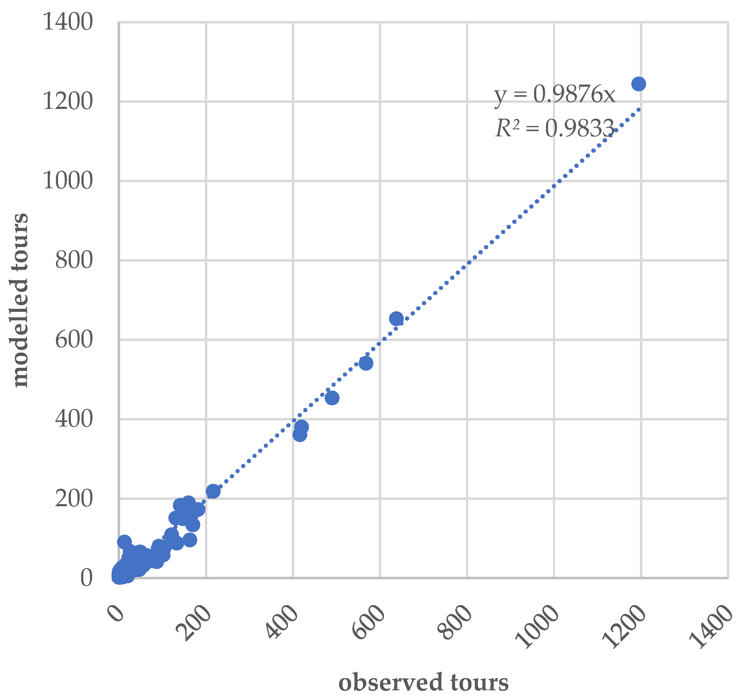
4.4. Validation Results

Once the model has been specified and calibrated, its sensitivity in predicting changes was investigated. In this way, the aim of this section is to apply the calibrated model (Table 1) to other cities in order to check its goodness.

The above model is applied to the inner areas of six other provinces of the Veneto Region (

Table 3. Results of trip-chain order model for selected areas.

	Verona	Rovigo	Venice	Treviso	Vicenza	Belluno
Attributes
Wholesale employees	9463	2112	3727	6597	7675	1270
Population	324,079	142,400	298,938	289,914	349,590	74,206
Average distance [km]	106.84	94.1	84.9	86.2	79.3	130.2
Tours
Tours per day (observed)	1083	976	2167	1558	1957	744
Tours/wholesale employees-day	0.114	0.462	0.581	0.236	0.255	0.586
Tours/population-day	0.003	0.007	0.007	0.005	0.006	0.010
Tours/average distance	10.14	10.37	25.54	18.07	24.69	5.71
Stop number class
Class 1	11.13%	14.00%	19.62%	15.66%	17.78%	8.46%
Class 2	13.19%	12.84%	13.95%	15.21%	16.42%	8.58%
Class 3	9.36%	14.77%	13.14%	12.07%	11.57%	12.32%
Class 4	66.32%	58.39%	53.30%	57.07%	54.23%	70.65%

) for which the number of tours generated was obtained from previous studies [8,9]. In terms of the number of stops per tour, the model reproduces quite well the distribution of tours departing from the investigated areas, e.g., for Treviso, the maximum difference between modelled and revealed shares is less than 5%. When travel distance increases in the distribution network, fewer direct tours (e.g., Belluno) and fewer tours in class 2 are predicted. Longer travel distance from the areas to serve leads to higher transportation costs; therefore, wholesalers indicate distance savings, which may be achieved by combining the location of their warehouses closer to the areas to serve and in low-congestion ones. In addition, to gain insight into the activity of freight vehicles and its impact on city traffic, the tours driving and the corresponding parking time requirements can be explored. It is important to note that parking time requirements represent the parking demand, while the number (and type) of parking available in the city represents the parking supply. Below, we refer to the demand side and not the supply side of parking space. It emerges that the stopping time for delivering depends on the number of tours performed (

Table 4. Average parking and delivering times.

Stop Number Class	Average Total Stop Time [Minutes]	Average Tour Time [Minutes]
Class 1	12.40	247.09
Class 2	114.80	255.29
Class 3	91.48	292.11
Class 4	84.95	280.54

).

The results are revealing. The most notable findings (

Table 5. Parking demand.

	Verona	Rovigo	Venice	Treviso	Vicenza	Belluno
parking demand (tours produced)
Class 1	1495	1694	5272	3025	4315	780
Class 2	16,399	14,387	34,704	27,204	36,890	7328
Class 3	9273	13,187	26,048	17,203	20,713	8385
Class 4	61,015	48,412	98,118	75,533	90,156	44,653
Total [minutes]	88,182	77,680	164,142	122,966	152,074	61,147
Total [h]	1469.7	1294.7	2735.7	2049.4	2534.6	1019.1

) are that tours consume a large portion of the total vehicle-hours for delivering and the share of stop time varies with the low values of round trips (i.e., 5%). We can see that as the number of stops increases, the time spent for at-customer operations decreases, with an incidence for longer tours of about 30%.

As shown in Table 5 and Figure 6, tours increase with population. Such a trend is understandable as also confirmed by investigation by Holguín-Veras et al. [45,46]. In areas with high population density, the shops tend to be smaller, with few spaces for storage. This produces a higher number of tours and stops given that smaller deliveries are performed and during the same travel more than one customer is served.

Expressed in relation to the distance from the area to serve, the total time spent in parking decreases as the distance rises. This result does not stand in contrast to what is expected given that longer tours consist of tours with many stops and subsequently low shipment size, which requires a short time to be delivered.

5. Conclusions

This paper presented some developments in delivery tour analysis in order to calibrate a model to evaluate the number of tours starting from a traffic zone. In particular, a discrete choice model was calibrated using FCD related to light freight vehicles.

The dataset for model calibration consists of more than 8520 tours undertaken in 60 days from the province of Padua. Some specific aspects of tour patterns are considered, such as the number of trips per tour (it emerged that about 24% of tours are composed of two trips) and tour distribution by time interval (20% of tours start from 7:00 to 8:00). Finally, considering the four classes of tours (in relation to the number of stops per tour) a first calibration of a model able to foresee the number of tours starting from an origin zone was developed. The calibrated model is a logit model where the utility function is expressed as a linear combination of the following attributes: the number of wholesalers and the population in the origin zone, the (average) distance between the origin zone and the other zones in the study area. Besides this, the model has been calibrated by considering different classes in terms of the number of stops with a coincidence ratio between observed and modelled tours that ranges from −3% to +18%. To gain insight into the overall volume of freight traffic in real-life environments, the model was used to quantify the total freight delivery tours of the other six provinces of the Veneto Region, which have various sizes. The resulting estimates were used to obtain comparative statistics.

One of the most important findings of this study refers to parking demand. Using the parking duration data collected, the paper analyzed the stop duration patterns and compared them to the total tour duration ones. The parking needs of freight vehicles are more than proportional to their traffic. This implies that allocating curbside space to that generic class of vehicles on the basis of their total traffic (under the assumption that freight vehicles follow shorter duration patterns than passengers in the peak hours) is bound to underestimate the space needs.

A further development of this study germinates from such findings: improving the results and applying more advanced machine-learning techniques that allow further features to be included in model specification and modelling accuracy to be improved. Further investigations should cover the influence of socio-economic attributes (such as retail size) on tour definition, and departure time choice vis-à-vis the relationship with time window access restrictions.

References

1. Nuzzolo, A.; Comi, A. Urban Freight Demand Forecasting: A Mixed Quantity/Delivery/Vehicle-Based Model. Transp. Res. Part E Logist. Transp. Rev. 2014, 65, 84–98. [Google Scholar] [CrossRef]
2. Kitamura, R.; Fujii, S.; Pas, E.I. Time-Use Data, Analysis and Modeling: Toward the next Generation of Transportation Planning Methodologies. Transp. Policy 1997, 4, 225–235. [Google Scholar] [CrossRef]
3. Dodson, J.; Burke, M.; Evans, R.; Gleeson, B.; Sipe, N. Travel Behavior Patterns of Different Socially Disadvantaged Groups: Analysis of Household Travel Survey Data for a Dispersed Metropolitan Area. Transp. Res. Rec. 2010, 2163, 24–31. [Google Scholar] [CrossRef]
4. Ezquerro, S.; Romero, J.P.; Moura, J.L.; Benavente, J.; Ibeas, Á. Minimizing the Impact of Large Freight Vehicles in the City: A Multicriteria Vision for Route Planning and Type of Vehicles. Available online: https://www.hindawi.com/journals/jat/2018/1732091/ (accessed on 1 December 2020). [CrossRef] [Green Version]
5. Schuessler, N.; Axhausen, K.W. Processing Raw Data from Global Positioning Systems without Additional Information. Transp. Res. Rec. 2009. [Google Scholar] [CrossRef]
6. Ayazi, E.; Sheikholeslami, A. A Data Mining Approach on Lorry Drivers Overloading in Tehran Urban Roads. Available online: https://www.hindawi.com/journals/jat/2020/6895407/ (accessed on 1 December 2020).
7. Nuzzolo, A.; Comi, A. Tactical and Operational City Logistics: Freight Vehicle Flow Modelling. In Freight Transport Modelling; Ben-Akiva, M., Meersman, H., Van de Voorde, E., Eds.; Emerald Group Publishing Limited: Bingley, UK, 2013; pp. 433–451. [Google Scholar] [CrossRef]
8. Nuzzolo, A.; Comi, A.; Polimeni, A. Urban Freight Vehicle Flows: An Analysis of Freight Delivery Patterns through Floating Car Data. Transp. Res. Procedia 2020, 47, 409–416. [Google Scholar] [CrossRef]
9. Comi, A.; Nuzzolo, A.; Polimeni, A. Aggregate Delivery Tour Modeling through AVM Data: Experimental Evidence for Light Goods Vehicles. Transp. Lett. 2021, 13, 201–208. [Google Scholar] [CrossRef]
10. Russo, F.; Comi, A. A Modelling System to Simulate Goods Movements at an Urban Scale. Transportation 2010, 37, 987–1009. [Google Scholar] [CrossRef]
11. Russo, F.; Vitetta, A.; Polimeni, A. From Single Path to Vehicle Routing: The Retailer Delivery Approach. Procedia-Soc. Behav. Sci. 2010, 2, 6378–6386. [Google Scholar] [CrossRef] [Green Version]
12. Holguín-Veras, J.; Sánchez-Díaz, I.; Lawson, C.T.; Jaller, M.; Campbell, S.; Levinson, H.S.; Shin, H.-S. Transferability of Freight Trip Generation Models. Transp. Res. Rec. 2013, 2379, 1–8. [Google Scholar] [CrossRef]
13. Sánchez-Díaz, I. Modeling Urban Freight Generation: A Study of Commercial Establishments’ Freight Needs. Transp. Res. Part Policy Pract. 2017, 102, 3–17. [Google Scholar] [CrossRef] [Green Version]
14. Hu, W.; Dong, J.; Hwang, B.; Ren, R.; Chen, Z. A Scientometrics Review on City Logistics Literature: Research Trends, Advanced Theory and Practice. Sustainability 2019, 11, 2724. [Google Scholar] [CrossRef] [Green Version]
15. Ambrosini, C.; Routhier, J.-L. Objectives, Methods and Results of Surveys Carried out in the Field of Urban Freight Transport: An International Comparison. Transp. Rev. 2004, 24, 57–77. [Google Scholar] [CrossRef]
16. Allen, J.; Browne, M.; Cherrett, T. Survey Techniques in Urban Freight Transport Studies. Transp. Rev. 2012, 32, 287–311. [Google Scholar] [CrossRef]
17. Hunt, J.D.; Stefan, K.J. Tour-Based Microsimulation of Urban Commercial Movements. Transp. Res. Part B Methodol. 2007, 41, 981–1013. [Google Scholar] [CrossRef]
18. Nuzzolo, A.; Comi, A.; Ibeas, A.; Moura, J.L. Urban Freight Transport and City Logistics Policies: Indications from Rome, Barcelona, and Santander. Int. J. Sustain. Transp. 2016, 10, 552–566. [Google Scholar] [CrossRef]
19. Thoen, S.; Tavasszy, L.; de Bok, M.; Correia, G.; van Duin, R. Descriptive Modeling of Freight Tour Formation: A Shipment-Based Approach. Transp. Res. Part E Logist. Transp. Rev. 2020, 140, 101989. [Google Scholar] [CrossRef]
20. Polimeni, A.; Russo, F.; Vitetta, A. Demand and Routing Models for Urban Goods Movement Simulation. Eur. Transp. 2010, 46, 3–23. [Google Scholar]
21. Musolino, G.; Rindone, C.; Polimeni, A.; Vitetta, A. Planning Urban Distribution Center Location with Variable Restocking Demand Scenarios: General Methodology and Testing in a Medium-Size Town. Transp. Policy 2019, 80, 157–166. [Google Scholar] [CrossRef]
22. Gómez-Marín, C.G.; Serna-Urán, C.A.; Arango-Serna, M.D.; Comi, A. Microsimulation-Based Collaboration Model for Urban Freight Transport. IEEE Access 2020, 8, 182853–182867. [Google Scholar] [CrossRef]
23. Wisetjindawat, W.; Sano, K.; Matsumoto, S.; Raothanachonkun, P. Microsimulation Model for Modeling Freight Agents Interactions in Urban Freight Movement. In Proceedings of the 86th Annual Meeting of the Transportation Research Board, Washington, DC, USA, 21–25 January 2007. [Google Scholar]
24. Ruan, M.; Lin, J.; Kawamura, K. Modeling Urban Commercial Vehicle Daily Tour Chaining. Transp. Res. Part E Logist. Transp. Rev. 2012, 48, 1169–1184. [Google Scholar] [CrossRef]
25. Outwater, M.; Smith, C.; Wies, K.; Yoder, S.; Sana, B.; Chen, J. Tour Based and Supply Chain Modeling for Freight: Integrated Model Demonstration in Chicago. Transp. Lett. 2013, 5, 55–66. [Google Scholar] [CrossRef]
26. Wang, Q.; Holguín-Veras, J. Tour-Based Entropy Maximization Formulations of Urban Freight Demand. In Proceedings of the 88th Annual Meeting of the Transportation Research Board, Washington, DC, USA, 11–15 January 2009.You, S.I.; Ritchie, S.G. Tour-Based Truck Demand Modeling with Entropy Maximization Using GPS Data. J. Adv. Transp. 2019, 2019, e5021026. [Google Scholar] [CrossRef]
27. Gonzalez-Calderon, C.A.; Holguín-Veras, J. Entropy-Based Freight Tour Synthesis and the Role of Traffic Count Sampling. Transp. Res. Part E Logist. Transp. Rev. 2019, 121, 63–83. [Google Scholar] [CrossRef]
28. Zhang, Z.; He, Q.; Tong, H.; Gou, J.; Li, X. Spatial-Temporal Traffic Flow Pattern Identification and Anomaly Detection with Dictionary-Based Compression Theory in a Large-Scale Urban Network. Transp. Res. Part C Emerg. Technol. 2016, 71, 284–302. [Google Scholar] [CrossRef]
29. Chankaew, N.; Sumalee, A.; Treerapot, S.; Threepak, T.; Ho, H.W.; Lam, W.H.K. Freight Traffic Analytics from National Truck GPS Data in Thailand. Transp. Res. Procedia 2018, 34, 123–130. [Google Scholar] [CrossRef]
30. Siripirote, T.; Sumalee, A.; Ho, H.W. Statistical Estimation of Freight Activity Analytics from Global Positioning System Data of Trucks. Transp. Res. Part E Logist. Transp. Rev. 2020, 140, 101986. [Google Scholar] [CrossRef]
31. Camargo, P.; Hong, S.; Livshits, V. Expanding the Uses of Truck GPS Data in Freight Modeling and Planning Activities. Transp. Res. Rec. 2017, 2646, 68–76. [Google Scholar] [CrossRef]
32. Karam, A.; Illemann, T.M.; Reinau, K.H.; Vuk, G.; Hansen, C.O. Towards Deriving Freight Traffic Measures from Truck Movement Data for State Road Planning: A Proposed System Framework. ISPRS Int. J. Geo-Inf. 2020, 9, 606. [Google Scholar] [CrossRef]
33. Romano Alho, A.; Sakai, T.; Chua, M.H.; Jeong, K.; Jing, P.; Ben-Akiva, M. Exploring Algorithms for Revealing Freight Vehicle Tours, Tour-Types, and Tour-Chain-Types from GPS Vehicle Traces and Stop Activity Data. J. Big Data Anal. Transp. 2019, 1, 175–190. [Google Scholar] [CrossRef] [Green Version]
34. Holguín-Veras, J.; Encarnación, T.; Pérez-Guzmán, S.; Yang, X. Mechanistic Identification of Freight Activity Stops from Global Positioning System Data. Transp. Res. Rec. 2020, 2674, 235–246. [Google Scholar] [CrossRef]
35. Du, J.; Aultman-Hall, L. Increasing the Accuracy of Trip Rate Information from Passive Multi-Day GPS Travel Datasets: Automatic Trip End Identification Issues. Transp. Res. Part Policy Pract. 2007, 41, 220–232. [Google Scholar] [CrossRef]
36. Wang, B.; Gao, L.; Juan, Z. A Trip Detection Model for Individual Smartphone-Based GPS Records with a Novel Evaluation Method. Adv. Mech. Eng. 2017, 9. [Google Scholar] [CrossRef] [Green Version]
37. Karam, A.; Illemann, T.M.; Reinau, K.H. GPS-Derived Measures of Freight Trucks for Rest Areas: A Case-Study Based Analysis. In Proceedings of the 2020 IEEE International Conference on Industrial Engineering and Engineering Management (IEEM), Marina Bay Sands, Singapore, 14–17 December 2020; pp. 939–943. [Google Scholar] [CrossRef]
38. Joubert, J.W.; Axhausen, K.W. Inferring Commercial Vehicle Activities in Gauteng, South Africa. J. Transp. Geogr. 2011, 19, 115–124. [Google Scholar] [CrossRef] [Green Version]
39. Comendador, J.; López-Lambas, M.E.; Monzón, A. A GPS Analysis for Urban Freight Distribution. Procedia-Soc. Behav. Sci. 2012, 39, 521–533. [Google Scholar] [CrossRef] [Green Version]
40. Yang, X.; Sun, Z.; Ban, X.J.; Holguín-Veras, J. Urban Freight Delivery Stop Identification with GPS Data. Transp. Res. Rec. 2014. [Google Scholar] [CrossRef]
41. Greaves, S.P.; Figliozzi, M.A. Collecting Commercial Vehicle Tour Data with Passive Global Positioning System Technology: Issues and Potential Applications. Transp. Res. Rec. 2008. [Google Scholar] [CrossRef] [Green Version]
42. Rathore, M.M.; Ahmad, A.; Paul, A.; Rho, S. Urban Planning and Building Smart Cities Based on the Internet of Things Using Big Data Analytics. Comput. Netw. 2016, 101, 63–80. [Google Scholar] [CrossRef]
43. Egu, O.; Bonnel, P. How Comparable Are Origin-Destination Matrices Estimated from Automatic Fare Collection, Origin-Destination Surveys and Household Travel Survey? An Empirical Investigation in Lyon. Transp. Res. Part Policy Pract. 2020, 138, 267–282. [Google Scholar] [CrossRef]
44. Ben-Akiva, M.; Lerman, S.R. Discrete Choice Analysis: Theory and Application to Travel Demand; Transportation Studies; MIT Press: Cambridge, MA, USA, 1985. [Google Scholar]
45. Holguín-Veras, J.; Jaller, M.; Sanchez-Diaz, I.; Wojtowicz, J.; Campbell, S.; Levinson, H.; Lawson, C.; Powers, E.L.; Tavasszy, L. Freight Trip Generation and Land Use; Transportation Research Board, National Academies of Sciences, Engineering, and Medicine, Ed.; The National Academies Press: Washington, DC, USA, 2012. [Google Scholar] [CrossRef]
46. Holguín-Veras, J.; Campbell, S.; González-Calderón, C.A.; Ramírez-Ríos, D.; Kalahasthi, L.; Aros-Vera, F.; Browne, M.; Sanchez-Diaz, I. Importance and Potential Applications of Freight and Service Activity Models. In City Logistics 1; John Wiley & Sons, Ltd.: Hoboken, NJ, USA, 2018; pp. 45–63. [Google Scholar] [CrossRef]
Figure 1. Study area and zoning.
Futuretransp 01 00038 g001
Figure 2. Tour pattern.
Futuretransp 01 00038 g002
Figure 3. Tour distribution by time interval from Padua.
Futuretransp 01 00038 g003
Figure 4. Number of trips per tour from Padua.
Futuretransp 01 00038 g004
Figure 5. Model validation: observed vs. modelled tours.
Futuretransp 01 00038 g005
Figure 6. Parking demand vs. distance of delivery location.
Futuretransp 01 00038 g006