
Advances in Regression Kriging-Based Methods for Estimating Statewide Winter Weather Collisions: An Empirical Investigation


Abstract
:1. Introduction and Background
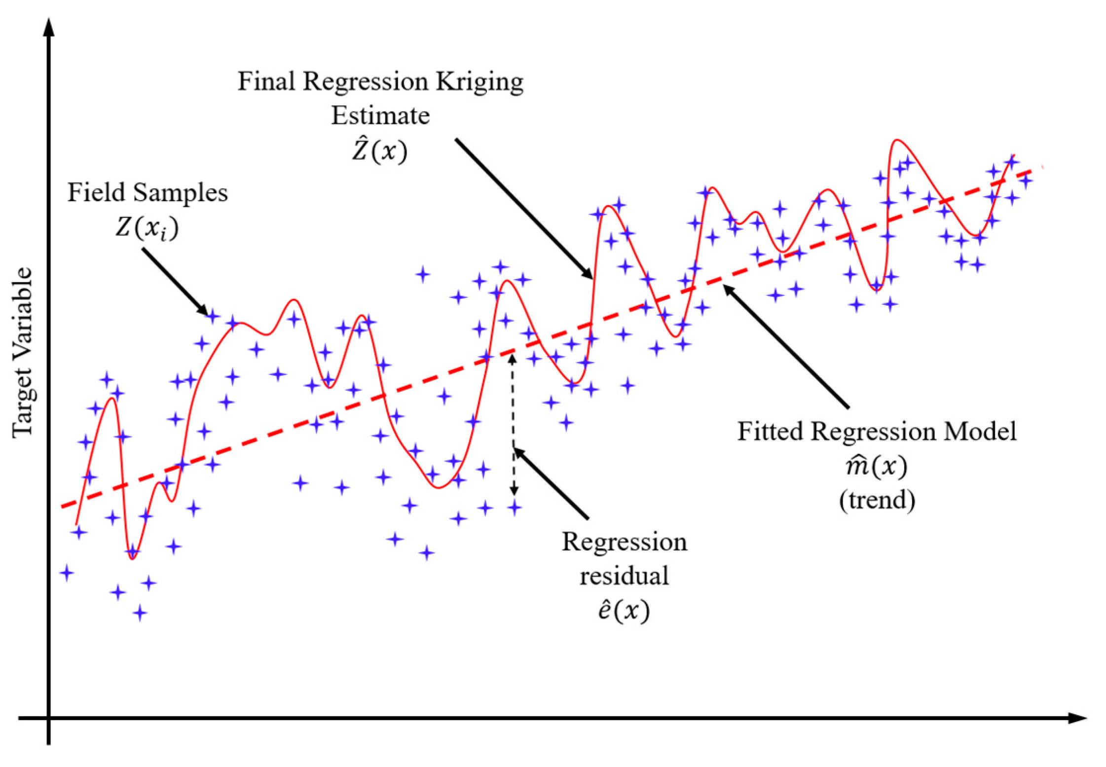
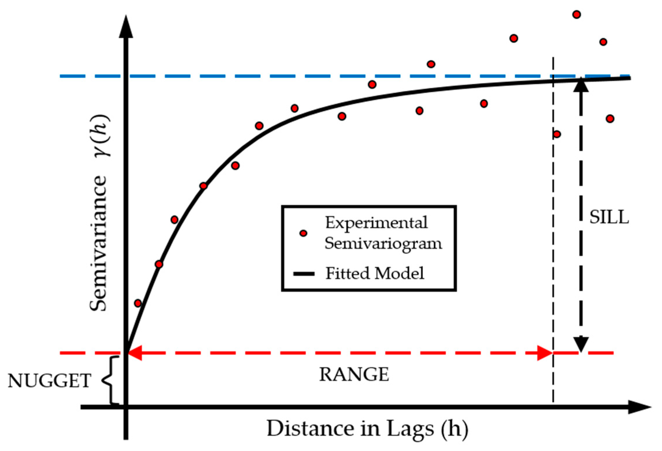
2. Regression Kriging Fundamentals
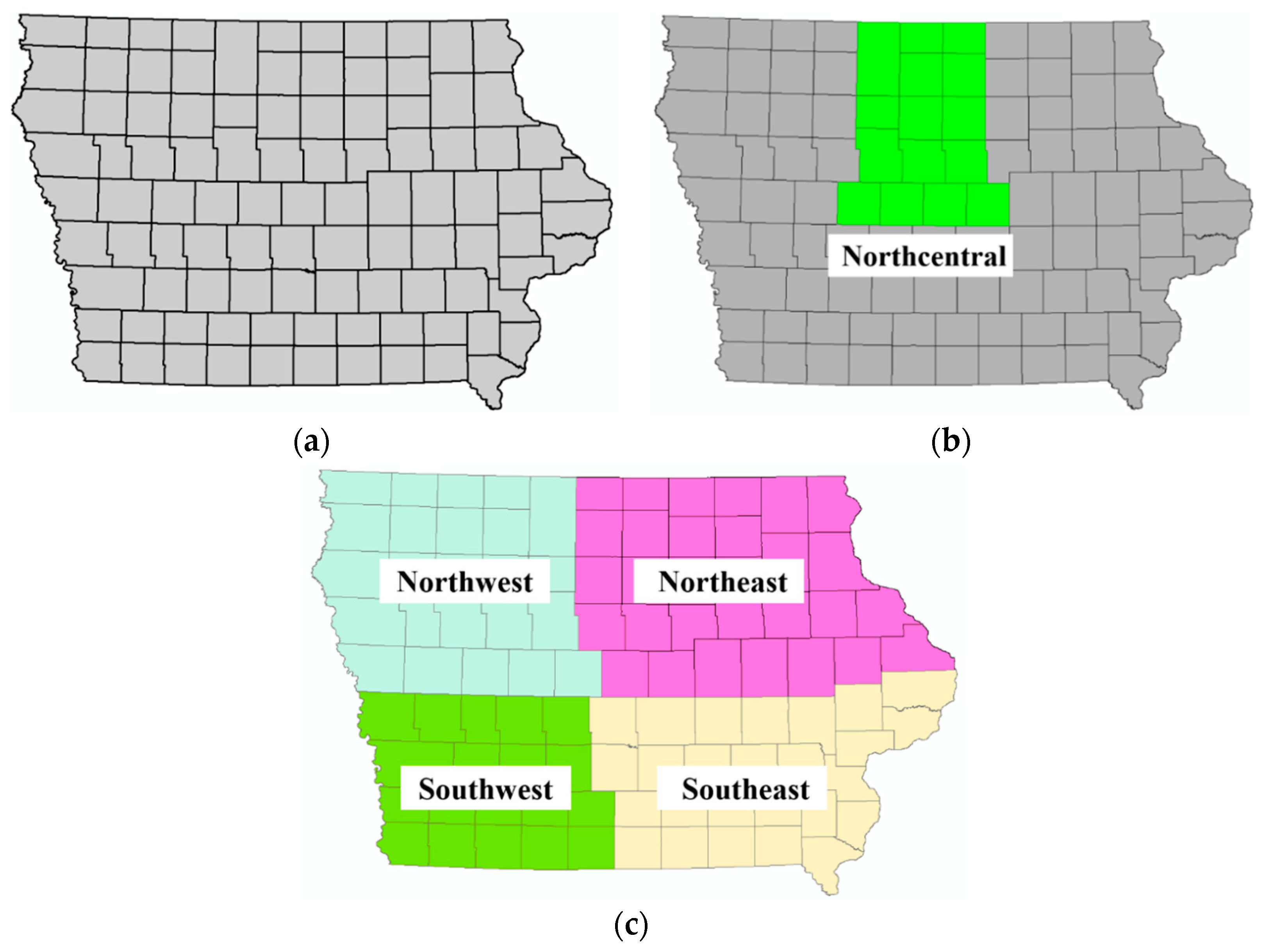
3. Study Area and Data
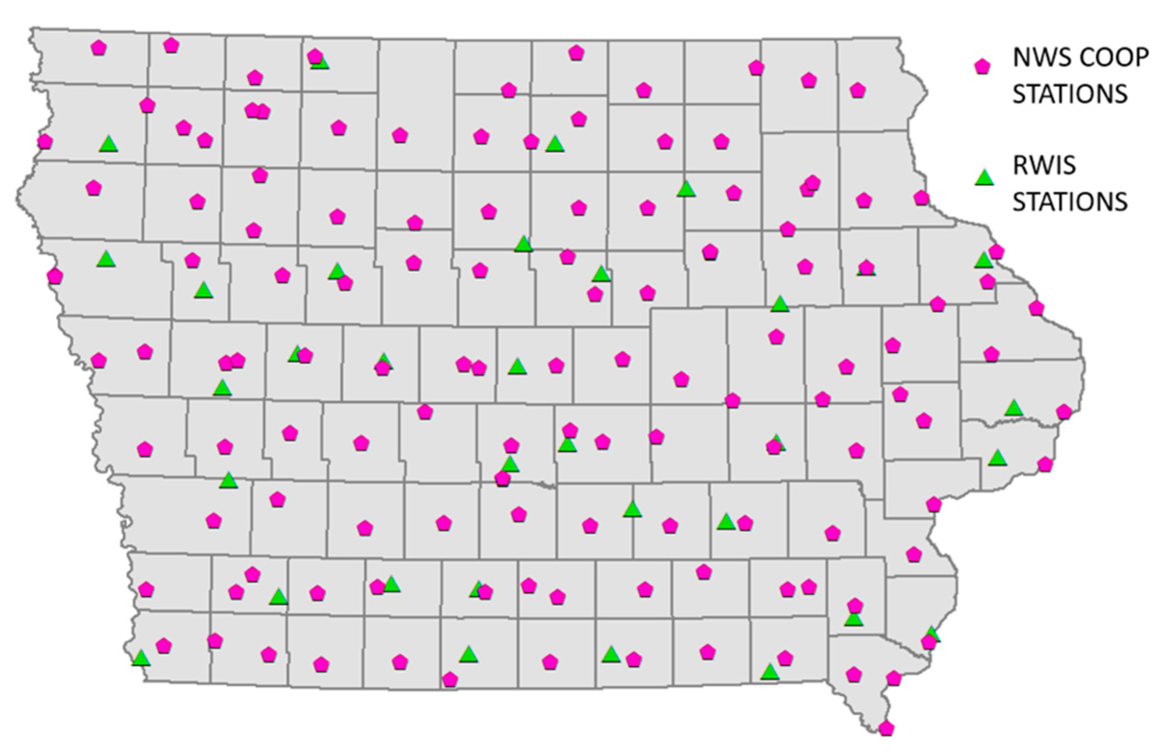
3.1. Meteorological and Road Conditions Data
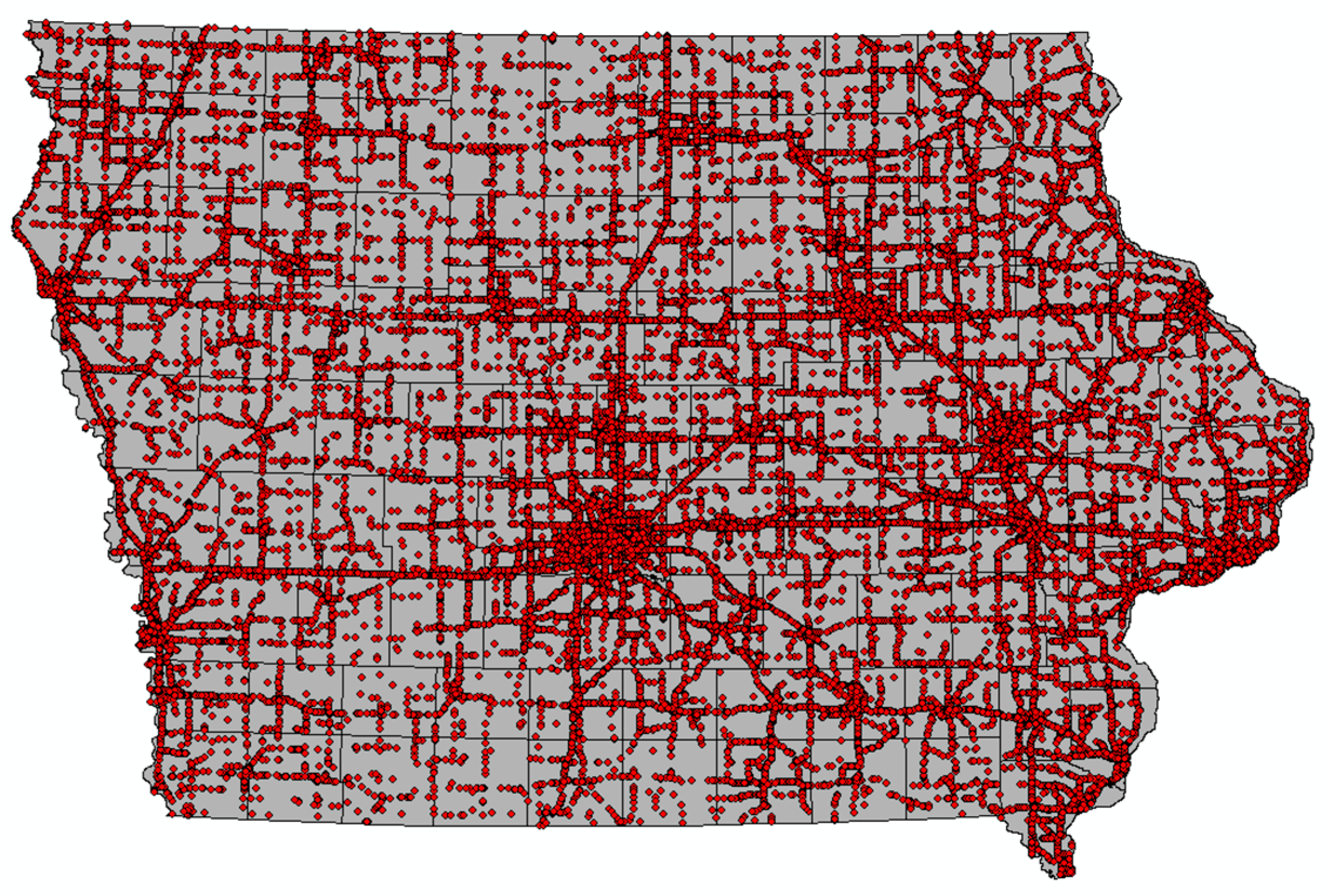
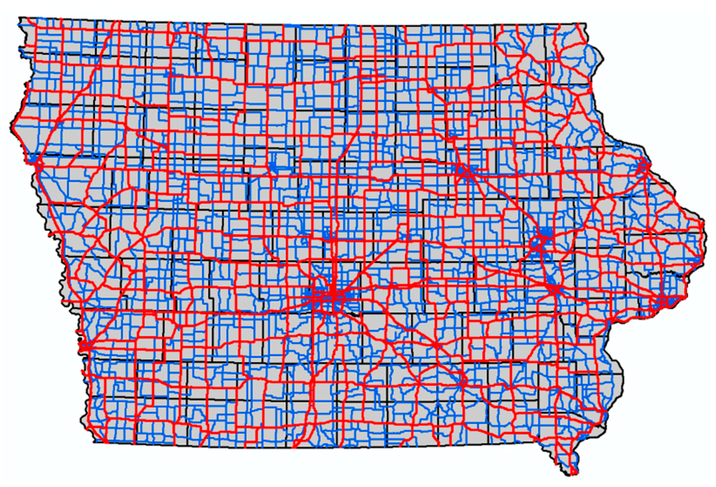
3.2. Road Network
3.3. Collision Data
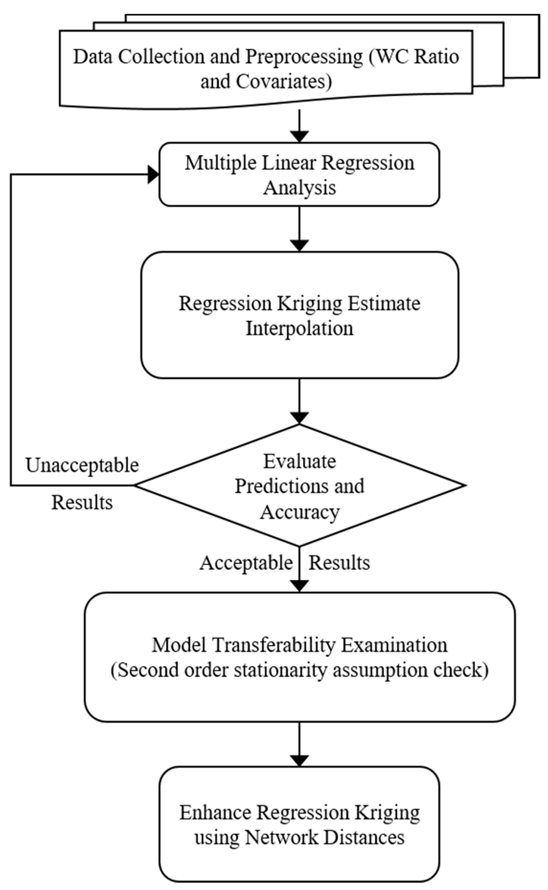
4. Methodology
4.1. Data Requirements
4.2. Spatial Interpolation via Regression Kriging (RK)
5. Results and Discussion
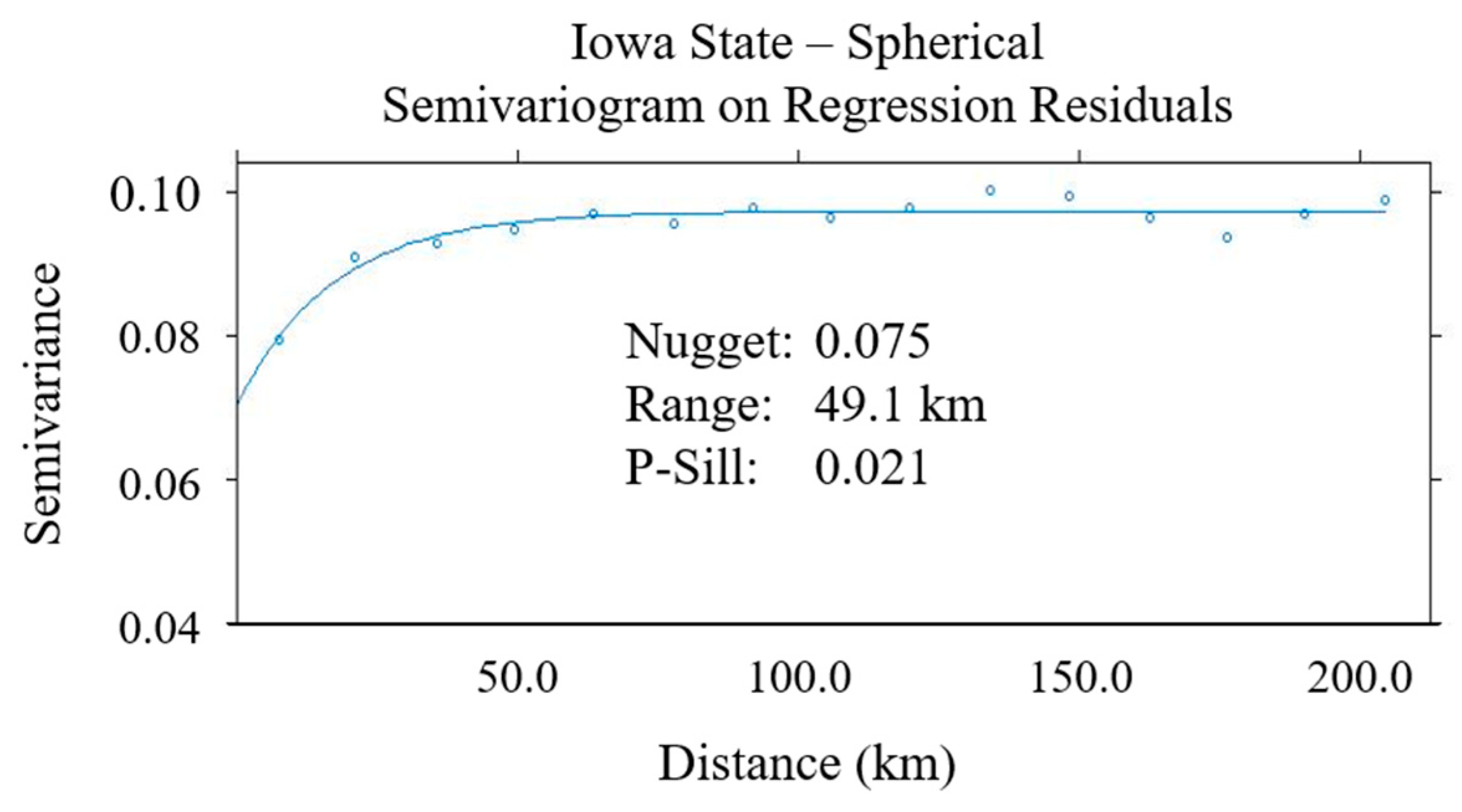
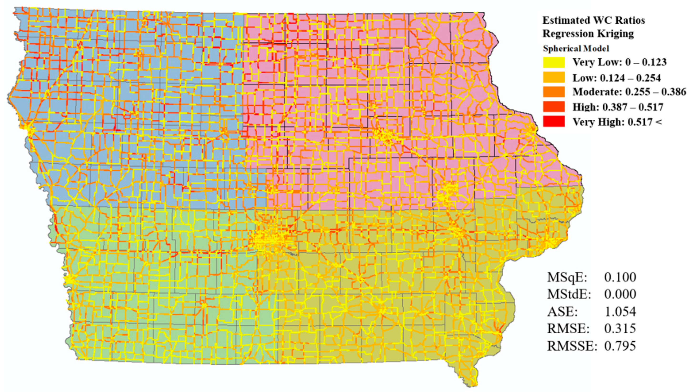
5.1. Development of A Statewide Regression Kriging Model
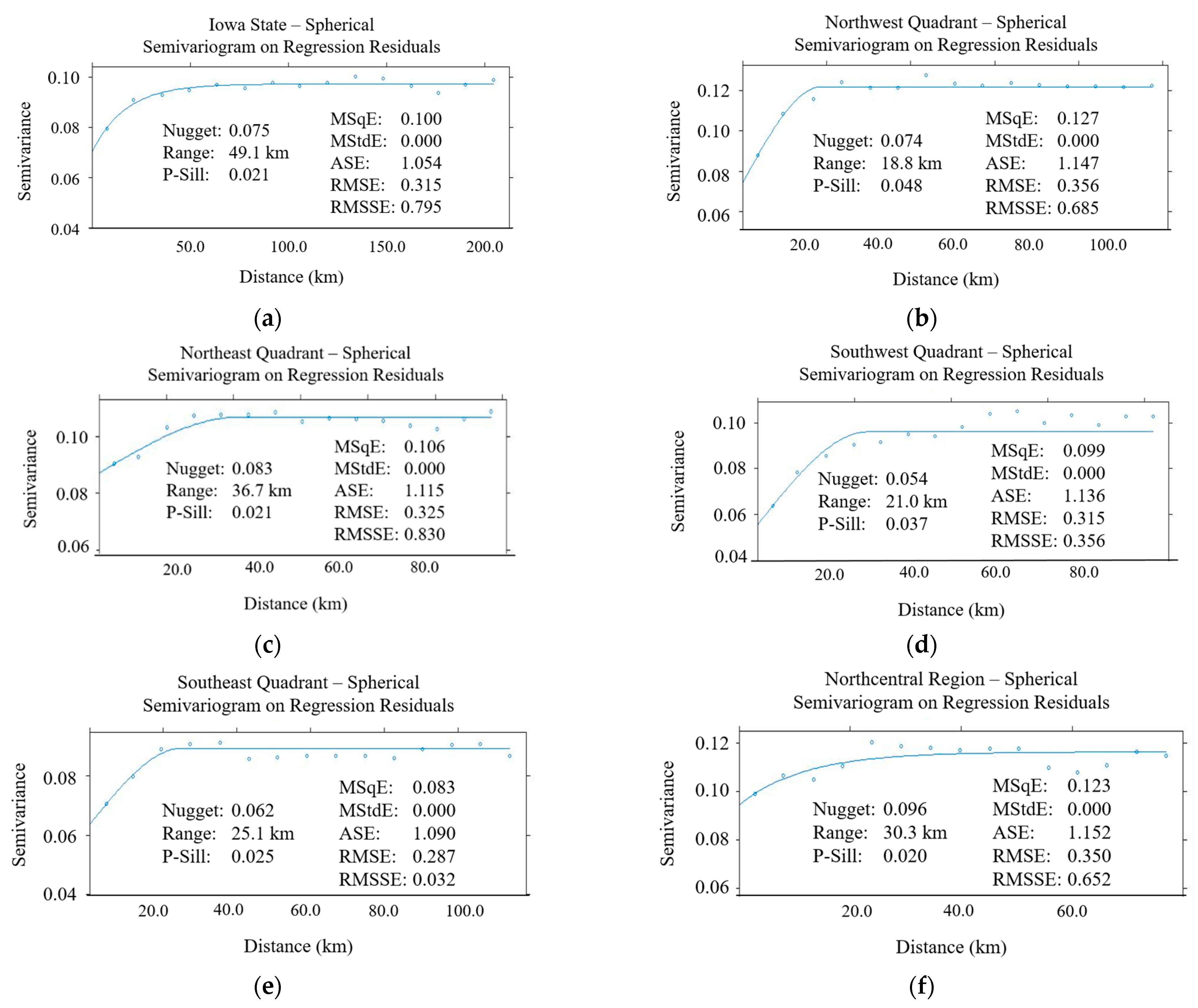
5.2. Validation of Model Transferability (Second Order Stationarity Assumption)
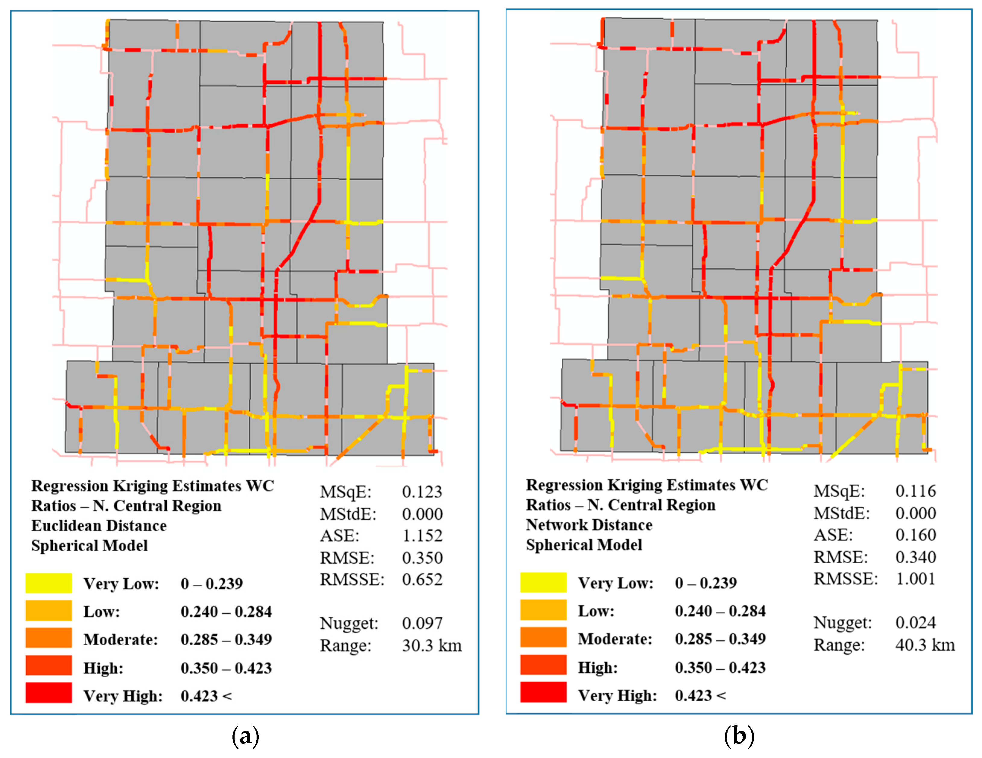
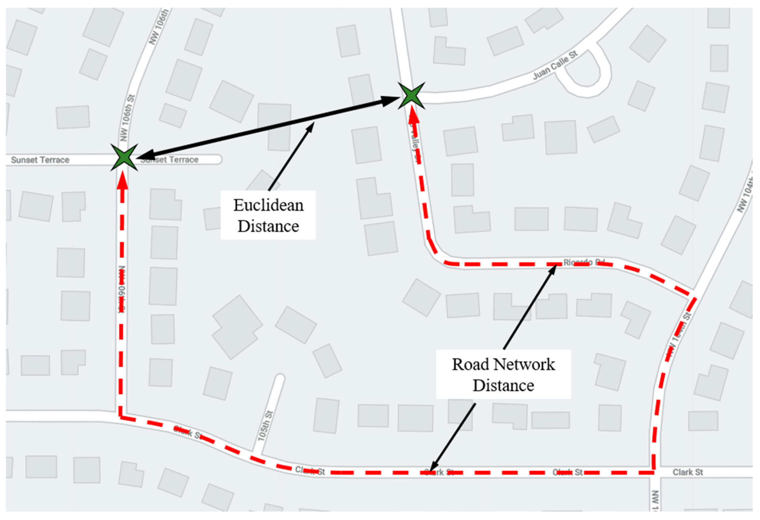
5.3. Network Regression Kriging Using Road Distances
6. Conclusions
- The regression analysis conducted for the six regions of the study area showed that not all covariates have the same effects within each region. Despite this, the results do support previous findings of factors that are connected to higher collision rates such as higher speed limits, less number of lanes, greater traffic volumes, and deteriorating road conditions. This shows how covariate selection itself is an important step worthy of its own project scope before applying it to regression kriging as it lays an important foundation for RK to build upon to further increase the estimation accuracy.
- The performance of regression kriging at a much larger scale with increased data quantity and density was found to be very robust based on the five statistical measures used. However, we found that the second order stationarity assumption did not hold, as the semivariogram and cross validation results for each of the six regions differed substantially. This also showed how the urban/rural setting of the region can greatly affect the model’s performance whereby rural road networks benefit from this process the most. However, an overall model is still adequate should higher fidelity not be required or if certain regions have insufficient data quality or quantity. This demonstrates how powerful a tool that RK can be for winter collision modelling.
- Finally, RK was enhanced by using road network distances over Euclidean distances. By the semivariogram value results and the five statistical measures, it was clear that RK with network distances outperformed its Euclidean distance counterpart. Applied over a large spatial scale, over a much larger and more complex connected road network, this study provides conclusive evidence that network distances can improve kriging estimation performance.
- One major assumption made is that the placement of the RWIS stations is optimal and substantially affects the outcome of weather induced collisions. The true effectiveness of RWIS and its warning system may provide insight into their effectiveness in reducing collisions, and its numerical valuation may be incorporated as a covariate.
- The study did not consider the effects of maintenance operations that could skew the collision frequencies being recorded. Incorporating maintenance characteristics, such as plowing schedules or chemical use, may further improve the regression portion of the analysis.
- This study used Iowa for its relatively uniform terrain characteristics, which may limit the results to more mountainous or hilly regions. Repeating this study, but in a different state or country altogether with drastically different geography, will further develop the process and also show if it can be applied universally or if regional adjustments are required.
- The datasets used are subject to human error and biases, especially for data that are recorded manually. Fortunately, environmental data is mostly automated now; however, collision and near-miss reports are not. The development and utilization of automated monitoring systems for collisions and near misses will reduce errors and biases while also providing the added variable of near misses.
- Expanding the weather source dataset and its quantity and quality may improve upon the environmental aspects of the modelling process. Additional covariates, such as dew point temperatures, visibility, or solar factors, may be considered.
Author Contributions
Funding
Institutional Review Board Statement
Informed Consent Statement
Data Availability Statement
Conflicts of Interest
References
- US DOT Federal Highway Administration. How Do Weather Events Impact Roads. 2020. Available online: https://ops.fhwa.dot.gov/weather/q1_roadimpact.htm (accessed on 25 July 2020).
- Royal Canadian Mounted Police. Just the Facts—Winter Driving. 2019. Available online: https://www.rcmp-grc.gc.ca/en/gazette/just-the-facts-winter-driving (accessed on 1 April 2021).
- Norrman, J.; Eriksson, M.; Lindqvist, S. Relationships between road slipperiness, traffic accident risk and winter road maintenance activity. Clim. Res. 2000, 15, 185–193. [Google Scholar]
- Heqimi, G. Using Spatial Interpolation to Determine Impacts of Snowfall on Traffic Crashes. Master’s Thesis, Michigan State University, East Lansing, MI, USA, 2016. [Google Scholar]
- Asano, M.; Hirasawa, M. Characteristics of traffic accidents in cold, snowy Hokkaido, Japan. In Proceedings of the Eastern Asia Society for Transportation Studies; Eastern Asia Society for Transportation Studies: Tokyo, Japan, 2003; Volume 4, pp. 1426–1434. [Google Scholar]
- Andersson, A.K. Winter Road Conditions and Traffic Accidents in Sweden and UK-Present and Future Climate Scenarios; Department of Earth Sciences, Institutionen för Geovetenskaper: Gothenburg, Sweden, 2010. [Google Scholar]
- American Association of State Highway and Transportation Officials (AASHTO). Highway Safety Manual, 1st ed.; AASHTO: Washington, DC, USA, 2010; Volume 1. [Google Scholar]
- Reyad, P.; Sacchi, E.; Ibrahim, S.; Sayed, T. Traffic conflict–based before–after study with use of comparison groups and the empirical Bayes method. Transp. Res. Rec. 2017, 2659, 15–24. [Google Scholar]
- Thakali, L.; Kwon, T.J.; Fu, L. Identification of crash hotspots using kernel density estimation and kriging methods: A comparison. J. Mod. Transp. 2015, 23, 93–106. [Google Scholar] [CrossRef] [Green Version]
- Selby, B.; Kockelman, K. Spatial Prediction of AADT in Unmeasured Locations by Universal Kriging; Transportation Research Record: Washington, DC, USA, 2011. [Google Scholar]
- Zhang, D.; Wang, X.C. Transit ridership estimation with network Kriging: A case study of Second Avenue Subway, NYC. J. Transp. Geogr. 2014, 41, 107–115. [Google Scholar] [CrossRef]
- Gu, L.; Kwon, T.J.; Qiu, T.Z. A Geostatistical Approach to Winter Road Surface Condition Estimation using Mobile RWIS Data. Can. J. Civ. Eng. 2019, 46, 511–521. [Google Scholar] [CrossRef]
- Zeng, Q.; Huang, H.; Pei, X.; Wong, S.C.; Gao, M. Rule extraction from an optimized neural network for traffic crash frequency modeling. Accid. Anal. Prev. 2016, 97, 87–95. [Google Scholar] [CrossRef] [PubMed] [Green Version]
- Abdelwahab, H.T.; Abdel-Aty, M.A. Development of artificial neural network models to predict driver injury severity in traffic accidents at signalized intersections. Transp. Res. Rec. 2001, 1746, 6–13. [Google Scholar] [CrossRef]
- Chang, L.Y. Analysis of freeway accident frequencies: Negative binomial regression versus artificial neural network. Saf. Sci. 2005, 43, 541–557. [Google Scholar] [CrossRef]
- Abellán, J.; López, G.; De OñA, J. Analysis of traffic accident severity using decision rules via decision trees. Expert Syst. Appl. 2013, 40, 6047–6054. [Google Scholar] [CrossRef] [Green Version]
- Das, A.; Abdel-Aty, M. A genetic programming approach to explore the crash severity on multi-lane roads. Accid. Anal. Prev. 2010, 42, 548–557. [Google Scholar] [CrossRef]
- Wong, A.H.; Kwon, T.J. Development and Evaluation of Geostatistical Methods for Estimating Weather-Related Collisions—A Large Scale Case Study. Transp. Res. Rec. 2021, 1–13. [Google Scholar] [CrossRef]
- Olea, R.A. Geostatistics for Engineers and Earth Scientists; Springer Science & Business Media: New York, NY, USA, 1999. [Google Scholar]
- Einax, J.; Soldt, U. Geostatistical and multivariate statistical methods for the assessment of polluted soils—merits and limitations. Chemom. Intell. Lab. Syst. 1999, 46, 79–91. [Google Scholar] [CrossRef]
- Cressie, N. The Origins of Kriging. Math. Geol. 1990, 22, 239–252. [Google Scholar] [CrossRef]
- Iowa Department of Transportation. Iowa DOT Open Data. Available online: https://public-iowadot.opendata.arcgis.com/ (accessed on 31 May 2020).
- Iowa State University. Iowa Environmental Mesonet. Available online: https://mesonet.agron.iastate.edu/ (accessed on 6 January 2020).
- De Pauw, E.; Daniels, S.; Brijs, T.; Elke, H.; Geert, W. The Magnitude of The Regression to the Mean Effect in Traffic Crashes; International Co-Operation on Theories and Concepts in Traffic Safety: Vienna, Austria, 2014. [Google Scholar]
- NOAA. Iowa Climate Normals Map. 16 May 2020. Available online: https://www.weather.gov/dmx/climatenormals (accessed on 16 May 2020).
- Eguía, P.; Granada, E.; Alonso, J.M.; Arce, E.; Saavedra, A. Weather datasets generated using kriging techniques to calibrate building thermal simulations with TRNSYS. J. Build. Eng. 2016, 7, 78–91. [Google Scholar] [CrossRef]
- Atkinson, P.M.; Lloyd, C.D. Mapping Precipitation in Switzerland with Ordinary and Indicator Kriging. J. Geogr. Inf. Decis. Anal. 1998, 2, 72–86. [Google Scholar]
- Khan, G.; Qin, X.; Noyce, D.A. Spatial Analysis of Weather Crash Patterns in Wisconsin. J. Transp. Eng. 2008, 134, 191–202. [Google Scholar] [CrossRef]
- NOAA, Climate Reports: February & Winter (Dec–Feb) 2015–2016. 2016. Available online: https://www.weather.gov/dvn/Climate_Monthly_02_2016 (accessed on 30 August 2021).
- NOAA, Climate Reports: February & Winter (Dec–Feb) 2016–2017. 2017. Available online: https://www.weather.gov/dvn/Climate_Monthly_02_2017 (accessed on 30 August 2021).
- ESRI. ArcGIS Desktop: Release 10; Environmental Systems Research Institute: Redlands, CA, USA, 2011. [Google Scholar]
- Microsoft. Excel 2016; Microsoft: Redmond, WA, USA, 2016. [Google Scholar]
- R Core Team. A Language and Environment for Statistical Computing; R Foundation for Statistical Computing: Vienna, Austria, 2020. [Google Scholar]
- Pebesma, E. Multivariable geostatistics in S: The gstat package. Comput. Geosci. 2004, 30, 683–691. [Google Scholar] [CrossRef]
- Van Rossum, G.; Drake, F.L. Python 3 Reference Manual; CreateSpace: Scotts Valley, CA, USA, 2009. [Google Scholar]
- Montgomery, D.C.; Peck, E.A.; Vining, G.G. Introduction to Linear Regression Analysis, 3rd ed.; John Wiley & Sons Inc.: New York, NY, USA, 2001. [Google Scholar]
- Oliver, M.A.; Webster, R. Basic Steps in Geostatistics: The Variogram and Kriging; Springer International Publishing: New York, NY, USA, 2015. [Google Scholar]
- Abdel-Aty, M.A.; Radwan, A.E. Modeling traffic accident occurrence and involvement. Accid. Anal. Prev. 2000, 32, 633–642. [Google Scholar] [CrossRef]
- El-Basyouny, K.; Sayed, T. Comparison of two negative binomial regression techniques in developing accident prediction models. Transp. Res. Rec. 2006, 1950, 9–16. [Google Scholar] [CrossRef]
- Usman, T.; Fu, L.; Miranda-Moreno, L.F. A disaggregate model for quantifying the safety effects of winter road maintenance activities at an operational level. Accid. Anal. Prev. 2012, 48, 368–378. [Google Scholar] [CrossRef] [PubMed]
- Wong, A.H. Advances in Kriging-Based Modelling Approaches of Winter Weather Vehicular Collisions—A Region-Wide Geostatistical Investigation. Master’s Thesis, University of Alberta, Edmonton, AB, Canada, 9 June 2021. [Google Scholar]


| Avg Mthly Road Surf Temp | Avg Mthly Air Temp | Avg Mthly Red Warnings | Avg Mthly Orange Warnings | Avg Mthly Yellow Warnings | Snowfall Totals | Avg Daily High Temp | Avg Daily Low Temp | |
|---|---|---|---|---|---|---|---|---|
| UNIT | °C | °C | Count | Count | Count | cm | °C | °C |
| MIN | −7.9 | −8.5 | 0 | 0 | 0 | 0 | −10.2 | −21.6 |
| MEAN | 2.7 | 1.0 | 100 | 875 | 30 | 5.1 | 5.4 | −5.5 |
| MAX | 14.9 | 14.8 | 990 | 2481 | 213 | 34.7 | 21.5 | 10.7 |
| STD DEV | 6.1 | 6.2 | 133 | 632 | 33 | 5.6 | 7.5 | 6.8 |
| STATION TYPE | RWIS | NWS COOP | ||||||
| No. OF STATIONS | 33 | 128 | ||||||
| Seasonal Collision Statistics | 2013–2014 Season | 2014–2015 Season | 2015–2016 Season | 2016–2017 Season | 2017–2018 Season | 5-Year Seasonal Totals | 5-Year Seasonal Average | Seasonal Std. Dev |
|---|---|---|---|---|---|---|---|---|
| Total Collisions | 22,178 | 21,529 | 22,821 | 22,264 | 22,907 | 111,699 | 22,340 | 557.4 |
| Total Winter Collisions | 7452 | 4911 | 4440 | 3912 | 5052 | 25,767 | 5153 | 1360.4 |
| Winter Collision Proportion | 33.6% | 22.8% | 19.5% | 17.6% | 22.1% | 23.1% | 23.1% | 6.2% |
| Total Fatal Collisions | 95 | 106 | 101 | 127 | 93 | 522 | 104 | 13.6 |
| Total Major Injury Collisions | 422 | 401 | 390 | 415 | 357 | 1985 | 397 | 25.6 |
| Total Minor Injury Collisions | 1744 | 1541 | 1700 | 1694 | 1673 | 8352 | 1670 | 76.8 |
| Total Possible Injury and PDO Collisions | 19,917 | 19,481 | 20,630 | 20,028 | 20,784 | 100,840 | 20,168 | 535.6 |
| Name | Formulation | Ideal Value |
|---|---|---|
| Mean Squared Error | Close to 0 | |
| Mean Standardized Error | Close to 0 | |
| Root Mean Squared Error | The smaller the value, the better the model | |
| Average Standardized Error | Close to RMSE | |
| Root Mean Squared Standardized Error | Close to 1 |
| Coefficient Values | Iowa State | Northwest | Northeast | Southwest | Southeast | North Central |
|---|---|---|---|---|---|---|
| Number of Data Points | 19,591 | 3257 | 6284 | 2565 | 7504 | 1090 |
| Adjusted R2 | 0.0355 | 0.0190 | 0.0389 | 0.0390 | 0.0182 | 0.0403 |
| Intercept | 0.1182 | −0.0839 | −0.4897 | −0.1691 | 0.0521 | −0.5572 |
| Number of Lanes | −0.0254 | na | −0.0217 | −0.0237 | −0.0305 | −0.0475 |
| Speed Limit | 0.0013 | 0.0015 | 0.0009 | 0.0020 | 0.0009 | na |
| ln(AADT) | 0.0165 | na | 0.0258 | 0.0220 | 0.0205 | 0.0470 |
| RST | −0.0418 | na | na | na | na | na |
| Avg. Air Temp | 0.0397 | na | na | na | −0.0300 | na |
| Seasonal Snowfall Total | na | 0.0558 | 0.0226 | na | na | na |
| No. of Red Warnings | na | −0.0004 | 0.0001 | 0.0014 | na | 0.0002 |
| No. of Orange Warnings | 0.00001 | na | 0.0002 | 0.0003 | na | 0.0005 |
| No. of Yellow Warnings | 0.0009 | na | 0.0040 | −0.0074 | 0.0010 | na |
Publisher’s Note: MDPI stays neutral with regard to jurisdictional claims in published maps and institutional affiliations. |
© 2021 by the authors. Licensee MDPI, Basel, Switzerland. This article is an open access article distributed under the terms and conditions of the Creative Commons Attribution (CC BY) license (https://creativecommons.org/licenses/by/4.0/).
Share and Cite
Wong, A.H.; Kwon, T.J. Advances in Regression Kriging-Based Methods for Estimating Statewide Winter Weather Collisions: An Empirical Investigation. Future Transp. 2021, 1, 570-589. https://doi.org/10.3390/futuretransp1030030
Wong AH, Kwon TJ. Advances in Regression Kriging-Based Methods for Estimating Statewide Winter Weather Collisions: An Empirical Investigation. Future Transportation. 2021; 1(3):570-589. https://doi.org/10.3390/futuretransp1030030
Chicago/Turabian StyleWong, Andy H., and Tae J. Kwon. 2021. "Advances in Regression Kriging-Based Methods for Estimating Statewide Winter Weather Collisions: An Empirical Investigation" Future Transportation 1, no. 3: 570-589. https://doi.org/10.3390/futuretransp1030030
APA StyleWong, A. H., & Kwon, T. J. (2021). Advances in Regression Kriging-Based Methods for Estimating Statewide Winter Weather Collisions: An Empirical Investigation. Future Transportation, 1(3), 570-589. https://doi.org/10.3390/futuretransp1030030