Towards Sustainable Liveable City: Management Operations of Shared Autonomous Cargo-Bike Fleets

Abstract

Finding a sustainable mobility solution for the future is one of the most competitive challenges in the logistics and mobility sector at present. Policymakers, researchers, and companies are working intensively to provide novel options that are environmentally friendly and sustainable. While autonomous car-sharing services have been introduced as a very promising solution, an innovative alternative is arising: the use of self-driving bikes. Shared autonomous cargo-bike fleets are likely to increase the livability and sustainability of the city, as the use of cargo-bikes in an on-demand mobility service can replace the use of cars for short-distance trips and enhance connectivity to public transportation. However, more research is needed to develop this new concept. In this paper, we investigate different rebalancing strategies for an on-demand, shared-use, self-driving cargo-bikes service (OSABS). We simulate a case study of the system in the inner city of Magdeburg using AnyLogic. The simulation model allows us to evaluate the impact of rebalancing on service level, idle mileage, and energy consumption. We conclude that the best proactive rebalancing strategy for our case study is to relocate bikes only between neighboring regions. We also acknowledge the importance of bike relocation to improve service efficiency and reduce fleet size.

1. Introduction

The move towards sustainable and livable cities has become urgent and is needed to ensure a better future for the next generation. One main issue in urban cities is street traffic. Policymakers, researchers, and companies are all investigating novel ways and solutions to make the city a better place for living, with less pollution, less congestion, and fewer accidents. Recently, the research has introduced the use of shared autonomous cars to reduce resources, energy consumption, and urban parking space [1,2]. The overarching promise is to provide the user with an on-demand, door-to-door trip enabling a new level of individual mobility. However, this idea is challenged by some recent studies demonstrating that such mobility services increase the mileage traveled in urban agglomerations and subsequently increase congestion and energy consumption [3,4]. Hence, fleets of autonomous cars, which are neither in private use nor in shared operation, would contribute to the sustainability or livability of a city. As Millard-Ball [5] points out, autonomous cars could even foster a move backwards in the direction of car-friendly cities, with strong street separations between cars and active modes of transport.

Most recent concepts of sustainable cities such as the human scale [6] or the 15 min city [7], in accordance with the New Urban Agenda [8], clearly show that the emphasis in urban planning is on calming streets, reducing the need for cars, promoting walking and biking, and enabling everyday activities such as meeting people, chatting, gardening, playing etc., to regularly occur on the streets. In this context, a solution was suggested to enhance the city’s sustainability, which consists of using a shared, autonomous cargo-bike fleet. Self-driving cargo bikes offer on-demand, door-to-door mobility through autonomous driving to the point of demand and can be also used for the first and last mile of public transportation (PT). This encourages people to cycle and pushes them to shift from cars to PT. They also improve the livability and sustainability of the city compared to shared autonomous vehicles (SAVs), as explained in Assmann et al. [9]. Indeed, shared autonomous cargo bikes allow for a reduction in street traffic through the use of cycling paths, as well as the space needed for parking, as bikes are generally smaller in size. In addition, autonomous bikes have the advantage that they can be driven manually when used by a passenger (the bike is powered through pedaling), contrary to SAVs, which are 100% based on autonomous driving. The manual drive allows for an important reduction in energy consumption, as long rides are defined as when a customer is using the bike. Furthermore, the cargo bike has the advantage of offering a storage space that allows for further substitutions of trips that would normally require a car (e.g., shopping, smaller transport). At present, cargo-bike sharing has shown a strong potential to reduce motorized traffic in a city [10,11]. In contrast to conventional bike-sharing, it enables the transport of errands, kids, equipment, and others. Therefore, it widens the scope of bike-sharing and enables a much higher substitution of motorized trips. Different companies and researchers have concentrated on the development of autonomous micro-vehicles and robots that can drive on sidewalks (and, subsequently, on mixed-used streets) and can be used for urban delivery [12]. These technologies have already been adopted for bikes, as Baum et al. [13] points out. In order to utilize the potential of cargo bike-sharing, it makes sense to integrate autonomous driving functionalities. This would enable the same on-demand, door-to-door service standards, utilize the potential to substitute car traffic, and widen the scope of conventional bike-sharing.

In this paper, we aim to study the use of autonomous bikes as a means of on-demand, shared-use, self-driving bikes services (OSABS). This system is currently under development by the authors and a research team at the University of Magdeburg [14]. It is based on the use of a three-wheeled electric cargo-bikes to ensure a good balance with the autonomous driving mode. The bike can be also used as an e-assisted bike in a manual mode. Figure 1 illustrates the basic concept of OSABS. A customer can request a bike via smartphone. The operation management (OM) center will choose a suitable bike (if available) for the customer’s request. The bike will autonomously ride to the point of demand within a given service time. The customer unlocks the bike and manually rides it to the desired destination. When they have arrived, the customer leaves the bike, and the OM center will decide on the next destination. The bike can drive autonomously to the next customer, a waiting station (to park close to future demands), or a charging station (for battery charging). The choice of the next task depends on the fleet management algorithms that were implemented. An optimized fleet management strategy allows for efficient coordination between demand and the bike fleet. It forms the necessary basis for a holistic evaluation of whether the concept of OSABS is economically viable in contrast with conventional bike-sharing and shared autonomous car fleets.

The aim of this work is to investigate fleet management strategies to find the best balance between customer satisfaction and cost reduction for OSABS. On the one hand, customers want quick and reliable access to bikes, which can result in a large fleet and frequent rebalancing. On the other hand, fleet operators are interested in the economic viability of their service, and consequently aim to reduce energy (mainly from idle traveling) and fleet costs as much as possible. Finding a favorable balance for both parties allows for the sustainable use of the service. To achieve this, we consider three different rebalancing strategies, paying particular attention to the tradeoffs facing fleet owners. Since OSABS is an entirely new system and there is no empirical data to evaluate the system, we chose the simulation study as our methodology to understand the operational insights of the system. Moreover, the simulation study provides fundamental knowledge about the interaction of various elements, improving and optimizing the architecture of complex systems. Therefore, to examine and evaluate the strategies on a meaningful scale, we implement them in an agent-based simulation model.

The remainder of this paper is organized as follows. In Section 2, we review a collection of the relevant publications on vehicle relocation problems. Section 3 describes the simulation environment and the developed relocation strategies. In Section 4, we present the results of the different tested scenarios. Section 5 discusses the simulation outcomes. Section 6 concludes by highlighting key findings and future research initiatives.

2. Literature Review

2.1. Vehicle Relocation Problem

The vehicle relocation (also called dispatching or rebalancing) problem is very widespread, and has different types in practice. Typical applications of vehicle rebalancing include car-sharing [15,16,17] and bike-sharing systems [18,19], Autonomous Mobility-on-Demand (AMoD) services [20,21], and emergency services (e.g., ambulances [22,23], police cars [24]). The formulation and resolution of the problem depend strongly on the context and the application field. For example, for ambulance relocation, this generally consists of solving a maximum coverage problem [25]. In addition, some constraints may exist, such as the fact that the ambulances are only relocated after serving a demand, and they are not allowed to move from one waiting location to another when empty [22]. For the conventional bike-sharing system, the dispatching problem mainly consists of relocating bicycles from oversupplied to undersupplied regions. A vehicle (usually a truck) should visit oversupplied stations (or points) to pick up bikes and drop them off in stations where there is a lack of bikes. The rebalancing (or repositioning) problem can be perceived as a pickup-and-delivery capacitated vehicle-routing problem [18]. The aim is to determine the best route for each truck and the number of bikes to load or unload at each visited station, so that we maximize the customer satisfaction in the overall system. We distinguish between four major categories of the repositioning problem [26,27]:

• The static and deterministic repositioning problem (SDRP): where all the inputs are known beforehand with certainty. This is the case for the bike relocation, which is operated overnight and does not integrate demand forecasting. It can be viewed as a static, many-to-many pickup and delivery problem. We can find a survey of the static bicycle repositioning problem in [28].
• The static and stochastic repositioning problem (SSRP): where the inputs arepartially known, with a defined probability. One example is the maximum expected covering problem (MEXCLP), which was applied to solve the relocation of medical service vehicles [29]. A probability function was included to consider the possibility that a requested vehicle is not available because of previous demands.
• The dynamic and deterministic repositioning problem (DDRP): where the problem is solved periodically (or in real-time) but the future input is unknown and there is no stochastic information. The value of inputs is known only when they appear. One example is the ambulance relocation problem solved by [30], where the dispatching problem should be solved each time a request appears.
• The dynamic and stochastic repositioning problem (DSRP): where the input is stochastic information, and the problem is solved in real-time. One application is the intraday bike-sharing rebalancing, which considers the upcoming demand during the day [31].

In our work, we consider a dynamic and stochastic problem where the future demand is available as a function of time. We also consider a station-based system. However, unlike the conventional bike-sharing system, no vehicle is needed to perform the rebalancing task. Our bikes can drive autonomously from one station to another to meet the upcoming demand. From the management perspective, the operation of our system could be compared to autonomous car fleets, mainly as a part of the AMoD services. For this reason, we will focus on the literature on on-demand autonomous vehicles, as the relocation operation is similar to our service.

2.2. Shared Autonomous Vehicles Fleet Management

With the growing popularity of shared mobility services and the fast advancement of autonomous-driven technology, there is an increasing research interest in the fleet management of SAV services. Hence, multiple studies in the literature attempt to investigate different strategies and policies. For a taxonomy on SAV fleet management problems, the reader can refer to [32]. In this work, we mainly focus on research that can be adapted to our case study. According to Narayanan et al. [33], we could classify SAV systems based on three characteristics: (i) booking type (ii) sharing system, and (iii) integration type. According to this classification, OSABS is a part of the on-demand, shared-use independent services. In this section, we review papers that examine similar systems to OSABS, typically autonomous mobility, on-demand (AMoD) services.

The autonomous driving technology opens up new opportunities for AMoD services to dynamically manage their fleets. One major challenge is the adequate distribution of the fleet of vehicles with the customer demand, which is usually asymmetric across the network and over time. Consequently, it is necessary to relocate idle vehicles according to future demand to guarantee service availability. However, complete information about upcoming requests is not granted. Thus, historical data are generally used to obtain statistical information that allows for an estimation of future demand. According to Weikl and Bogenberger [34], we can differentiate between two main rebalancing strategies:

• User-based strategies: for this type, the customer is given incentives to move from an area of high demand to an area of low demand where there is an offer. These incentives could be a free ride, a lower price, or extra free time.
• Operator-based strategies: these consist of relocating vehicles with the intervention of the system manager. The rebalancing operation is performed based on a criterion reflecting the statistics calculation of demand and supply in the different stations or areas in the system. The criteria could be, for example, the number of available and needed vehicles, a calculated index, or waiting times. These strategies are the most studied in the literature. We can find various papers with different assumptions regarding the type of network, reservation structure, and fleet characteristics. Many studies consider a grid network, where the operating area is devided into blocks and the imbalance of each block is evaluated. Thereafter, vehicles should move from surplus blocks to deficit blocks. Fagnant and Kockelman [35] implemented four strategies in a subsequent order for each relocation period. First, they spread idle vehicles according to block balance. Second, they moved excess idle vehicles (any with more than two per zone) to zones unoccupied by idle vehicles. Chen et al. [36] built from the framework in [35] to investigate the operations of a SAV fleet under various vehicle range and charging infrastructure assumptions. Winter et al. [20] simulated an AMoD service on a generic grid network to study the impact of five different rebalancing policies for idle vehicles on parking needs, passenger waiting time, and empty mileage. The limit of such a network is that the traveling cost is roughly estimated. They assume that vehicles move from one grid to another at a fixed cost. Other papers consider a graph network where stations are nodes and the edges represent the traveling cost. Spieser et al. [37] extended a linear program formulation from [38] to compare the relocation that only responds to the current state of the system, the relocation that integrates future demand estimation, and the relocation with certain demand information. The demand destination is assumed to be known. Tsao et al. [39] studied the rebalancing of an AMoD system with uncertain travel demand forecasts. They formulated the problem as an integer program and developed a relaxed approach to solving it. Azevedo et al. [40] solved a linear program each hour to find the number of vehicles that move from an oversupplied station to an undersupplied station while minimizing the traveling cost. These different models mainly concern the periodic relocation, which occurs in each defined period T, and ignores the possible relocation between periods when a vehicle becomes idle.
  To the best of our knowledge, only two papers were found where a road network was used. Wallar et al. [41] presented a method to divide the operating area into a set of relocation regions and estimate the demand in each region. The rebalancing algorithm optimizes the relocation of idle vehicles between these regions using integer linear programming. Marczuk et al. [42] adopted the same formulation as in [40] to analyze the importance of rebalancing the system fleet size and the customer waiting time.
  Few papers considered a real network (maps) in their simulation. Winter et al. [21] used the map from Open Street Map (OSM) and compared three proactive rebalancing heuristics for SAVs under parking constraints. Brendel et al. [43] used Google Maps to examine and adapt existing carsharing rebalancing policies for SAVs. They combined operation-based relocation (ObR) strategies (relocation between stations) and user-based relocation (UbR) strategies (relocation after rental) in one model to show the positive impact of UbR on the number of served customers.

To conclude, there are many publications on relocation algorithms for autonomous vehicles, and there are also many attempts to simulate such services. To date, all of them use specific simplifications and assumptions, mainly regarding the network type, the routing, and the demand profiles. In summary, those assumptions include the following points:

• Most papers only evaluate periodic relocation. The immediate relocation after rental is considered in only one paper, with the limitation that only one rebalancing operation is possible for the bike when it becomes idle (either periodic or after rental). In this paper, we extend the work of Brendel et al. [43] by allowing for multiple rebalancing operations for the bike.
• Many studies consider open requests, where the customer demand never quits the system if it is not fulfilled. We assume that this representation cannot reflect the real-world case, as the customer cannot wait for too long. In our simulation model, we reject each request that cannot be satisfied within a 10 min waiting time.
• Vehicle routing is not explicitly simulated on a real road network but roughly estimated in a regional manner. Most papers work on a complete graph with a relatively small number of nodes. In this work, we use a detailed routing with a real road network, based on an Open Street Map. Unlike the SAVs, our bikes use the bicycle lanes and have a limited speed of 25 km/h. In addition, each routing mode (manual and autonomous mode) has its own requirements. Thus, we developed our specific routing calculation according to the system requirements.
• For SAVs, the destination of the customer at the time of renting the vehicle is assumed to be known, as the customer books a defined trip. This facilitates fleet optimization and the calculation of the fleet imbalance for the coming period. In our case, the customer books a bike. The trip duration and the customer’s destination are unknown till the customer leaves the bike.
• Operational constraints, such as parking and recharging, are rarely simulated, as in this work.
• The demand profiles used are generally computer-generated demands, which do not accurately capture the complex distribution of origins and destinations in a real transport system. In this work, a detailed population-based demand pattern is used, which imitates the real biking demand in high temporal and spatial detail.
• Small demand and fleet sizes are mostly used in the simulation scenario to manage computational time. Those scalings have unclear effects on the accuracy of the results. In this work, we simulate full demand and calculate the needed fleet size.

The contribution of this work is the development and evaluation of various fleet management strategies, which capture these different assumptions. The comparison of different policies allows for a better understanding of our system and helps to choose an adequate strategy. With the long-term goal of proving the economic viability of OSABS, it is important to perform the rebalancing operation efficiently, in order to avoid unnecessary costs.

3. Simulation Setup

This section describes the simulation environment in which our developed fleet management strategies will be evaluated.

3.1. Demand Generation

Fleet management strategies for autonomous fleets are generally evaluated in simplified graphs. Thus, their transferability to possible real-world applications is limited, due to a lack of realism in the routing and demand input. We aim to overcome this by basing our simulation on a real-world city with its original street network. The city of choice for our evaluations is the city of Magdeburg, Germany. This is a medium-sized city which, on the one hand, is big enough to represent the different urban forms of a city. On the other hand, it is not too large, keeping computing efforts on a reasonable scale. We will simulate OSABS in this operational area. For this purpose, we need to define the demand for trips with autonomous cargo bikes.

Several approaches in the literature provide a framework for the creation of demand scenarios for conventional bike-sharing systems. According to [44], these models can be grouped into two main categories: demand rebalancing and demand forecasting models. The latter can be further divided into city-level (e.g., [45]), cluster-level (e.g., [46]), and station-level (e.g., [47]) demand prediction models [48]. However, a major proportion of these models uses the existing data of already-implemented conventional bike-sharing systems to predict demand in the given system. There are approaches to introduce bike-sharing systems in cities where such systems do not yet exist [49,50]. Still, OSABS include some particularities, making it difficult to compare them with existing systems.

Therefore, we developed an approach to determine the demand for the new mobility concept in a temporally and spatially disaggregated manner. We then applied this to the city of Magdeburg. In the first step, a survey of mobility needs is conducted and evaluated concerning the city-wide usage potential of autonomous cargo bikes. The potential is calculated as usage likelihood, expressed as a modal split for the entire city. In our case, the survey is for the city of Magdeburg and provided us with the probability that road users replace each conventional mode of transport (cars, foot, bike, public transport) with OSABS. In addition, the survey was used to determine the distance that respondents would be willing to travel with an autonomous cargo bike.

Secondly, the resulting usage likelihood is spatially disaggregated. For spatial disaggregation, we used existing traffic data from well-established and widely used traffic demand models. According to [51], cross-section counts were carried out to determine the composition and distribution of traffic volumes. This involves recording the vehicles or people that pass through a specific area during a defined survey period. To ensure a representative representation of the traffic situation, such surveys were carried out on specific survey days: Tuesday and Thursday. The other days were unsuitable because there are comparatively high traffic volumes (Monday and Friday) or some service areas are closed in the afternoon or all day (Wednesday, Saturday, and Sunday) (see [51]). These survey days are also referred to as normal working days or statistical traffic days. For our purpose, the traffic data were provided by the municipality of Magdeburg. The data were available in the form of origin–destination pairs (OD pairs) for four different modes of transport per statistical traffic day. The OD pairs describe both the traffic flow between the individual zones (interzonal flow) and the traffic flow within the respective traffic zone (intrazonal flow). In our case, those are statistical zones of approx. 80,000 inhabitants. We used the modal split and stated distance limits to calculate the OSABS demand of each OD pair. Thus, we can calculate the traffic volumes of autonomous cargo bikes between all zones for one statistical day.

In our third step, the resulting demand between the OD pairs is temporally disaggregated. This was carried out to enable the prediction of usage per hour. For this purpose, we derived usage patterns from an existing conventional bike-sharing system in the city of Hamburg [52]. Since OSABS are still operated with bikes, we assumed similar usage patterns and applied them to the new system. Therefore, we derived both daily and weekly profiles for the use of the conventional bike-sharing system to temporally disaggregate the demand of a statistical day to the demand per hour, and distribute this over a week.

The resulting hourly distribution of bookings for each day of the week is shown in Appendix A (

Table A1. Hourly share of demand.

	Share
Time	Monday	Tuesday	Wednesday	Thursday
0–1	1.08%	1.21%	1.40%	1.67%
1–2	0.69%	0.72%	0.87%	1.03%
2–3	0.39%	0.37%	0.44%	0.60%
3–4	0.27%	0.23%	0.27%	0.39%
3–4	0.23%	0.16%	0.19%	0.26%
5–6	0.39%	0.35%	0.34%	0.37%
6–7	1.27%	1.38%	1.25%	1.28%
7–8	4.40%	4.98%	4.72%	4.55%
8–9	8.37%	9.24%	8.92%	8.54%
9–10	5.10%	5.49%	5.33%	5.26%
10–11	3.15%	3.15%	3.10%	3.11%
11–12	3.56%	3.43%	3.36%	3.50%
12–13	4.75%	4.71%	4.69%	4.85%
13–14	5.20%	4.97%	5.01%	5.13%
14–15	5.20%	4.87%	4.88%	5.03%
15–16	6.23%	5.82%	5.71%	5.89%
16–17	7.90%	7.47%	7.47%	7.42%
17–18	10.48%	9.98%	9.88%	9.50%
18–19	10.65%	10.14%	10.11%	9.66%
19–20	7.49%	7.23%	7.36%	7.18%
20–21	4.95%	5.04%	5.16%	5.00%
21–22	3.57%	3.78%	3.79%	3.75%
22–23	2.77%	3.08%	3.23%	3.27%
23–24	1.91%	2.19%	2.51%	2.78%
	Share
Time	Friday	Saturday	Sunday
0–1	2.09%	3.52%	3.69%
1–2	1.47%	2.97%	3.42%
2–3	0.93%	2.15%	2.65%
3–4	0.63%	1.53%	1.99%
4–5	0.41%	1.10%	1.50%
5–6	0.43%	0.80%	1.11%
6–7	1.16%	0.62%	0.82%
7–8	3.98%	0.78%	0.86%
8–9	7.43%	1.46%	1.29%
9–10	4.81%	2.69%	2.33%
10–11	3.16%	3.86%	3.57%
11–12	3.63%	5.27%	4.88%
12–13	4.94%	6.43%	6.41%
13–14	5.60%	7.33%	7.66%
14–15	5.94%	7.75%	8.42%
15–16	6.66%	7.77%	8.52%
16–17	7.82%	7.38%	8.28%
17–18	8.51%	7.48%	8.05%
18–19	7.93%	6.96%	7.08%
19–20	6.45%	6.22%	5.86%
20–21	5.18%	5.16%	4.24%
21–22	4.01%	3.98%	3.04%
22–23	3.48%	3.36%	2.48%
23–24	3.33%	3.43%	1.85%

). In addition to the time- and space-related influencing variables, seasonal effects were also taken into account when creating the demand for an entire year, since, according to [53], these have a significant influence on the use of bike-sharing systems. For this purpose, we extended the usage data of the conventional system with weather data. These include hourly data on temperature, precipitation and wind speed, and can be retrieved from the open-data portal of the German Weather Service (https://opendata.dwd.de/, accessed on 19 May 2021).

With the help of a regression analysis, we then determined the influence of the respective weather variables on the use of the bike-sharing system. Using these influencing factors and an arbitrary weather dataset, we could first model the influence of weather on daily or weekly OSABS demand. In addition, this allowed us to scale hourly demand between OD pairs as a function of the prevailing weather conditions over an arbitrarily long period of time. Thus, per OD pair, we could model the daily, weekly and yearly profile of OSABS demand, while the randomization of demand was possible through the application of different weather scenarios. The approach is summarized below in the form of a flowchart (Figure 2).

An extract of the resulting demand for a statistical traffic day is shown in Figure 3. The figure represents the hourly interzonal and intrazonal traffic flow between traffic zone 11 (city-center district with a high density of restaurants and pubs) and traffic zone 41 (university district). The upper bar chart describes the traffic flows starting from zone 15, while the lower chart describes the traffic flows starting from zone 41. In addition, Appendix A (Table A1) shows the hourly distribution of bookings for each day of the week.

3.2. Model Description

In order to understand the insights of the OSABS, we developed an agent-based simulation model using Anylogic based on our conceptual model presented in [54]. The developed conceptual model represents the key elements of OSABS, which are: demand scenarios, order management, operational aspects (bikes and stations), and output indicators where we calculate the performance indicators. Vasu Dev et al. [55] presented a detailed description of the simulation testbed for the OSABS. The process flow of the simulation model is as follows:

• Demand generation: we generated the demand data as an origin–destination pair for each region. We fed these demand data as an input to the simulation model, which schedules the customer arrivals. The customer arrives at a random location in the origin region. Then, the customer generates the request for the autonomous cargo bike with the constraints of a 10-min waiting time.
• Matching request: The matching algorithm receives the customer request and checks for available cargo bikes from the fleet near the customer location. It assigns the suitable cargo bike to the customer if available, based on the route calculation.
• Route calculation: The routing algorithm generates the best possible bike route for the selected bike to the customer. Anylogic has an inbuilt routing engine that can provide an online route for the bike. However, we developed a custom route provider using the Graphhopper routing engine to provide autonomous routing and manual routing for our cargo bike. Graphhopper is an open-source java routing engine, which parses OpenStreetMap data and allows for caluclation of the shortest path algorithm between two points [56]. Given two coordinations, GraphHoppers allows the best route for the chosen vehicle profile to be found, considering the chosen weight function. We developed two vehicle profiles, one for the autonomous mode and one for the manual mode, as the routes and the energy consumption differs between the two modes. For a reliable routing, we parsed the specific cycling paths our cargo bike can use using tGraphhopper, by avoiding footways, platforms, pedestrians, steps, and non-paved routes. We also defined the speed of the bike depending on the type of surface tag and highway tag in OSM. To calculate the best route, we implemented our own weighting function, which allows us to determine the route with less energy consumption.
• Bike movement: The cargo bike drives autonomously to the assigned customer. As the customer has the destination region information, the customer drives manually to the random destination location using the manual routing mode.
• Rebalancing: Once the customer reaches the destination, he or she drops the cargo bike. If there is a nearby request, then the bike moves directly to the next customer; otherwise, the chosen rebalancing strategy relocates the bike to the suitable waiting station.
• Output indicators: As an output of the simulation, we collect a list of statistics including the number of customer requests, the number of customers served, service level, time utilization of the cargo bike with the customer and without the customer, energy consumption during autonomous driving and manual driving.

This case study focuses on the autonomous cargo-bike sharing system. We consider the inner city of Magdeburg as the operational area, which contains 14 zones, named regions. The area chosen for our simulation was selected based on the real traffic data provided by the municipality of Magdeburg. Since the operational area is located in the city center, there is a high traffic density in combination with the traffic distribution, favoring the use of alternative mobility concepts.

Table 1. Traffic distribution in the operational area.

Distance d (km)	Share Distance (%)	Share Foot (%)	Share Bike (%)	Share Public Transport (%)	Share Car (%)
$0\le d<1$	18.32	75.26	9.54	9.95	5.24
$1\le d<2$	58.74	62.11	11.65	16.35	9.88
$2\le d<3$	12.84	39.52	18.29	27.36	14.82
$d\ge 3$	10.10	20.69	21.64	31.48	26.18

shows both the distribution of the distances traveled and the shares of the respective means of transport depending on the distance. As can be seen, the share of trips covered on foot is the highest. However, with increasing distance, the shares of other modes of transport, especially motorized individual transport and public transport, significantly increase. This can be observed for trips with a distance of more than one kilometer, whose share is notably larger compared to trips with a distance of less than one kilometer.

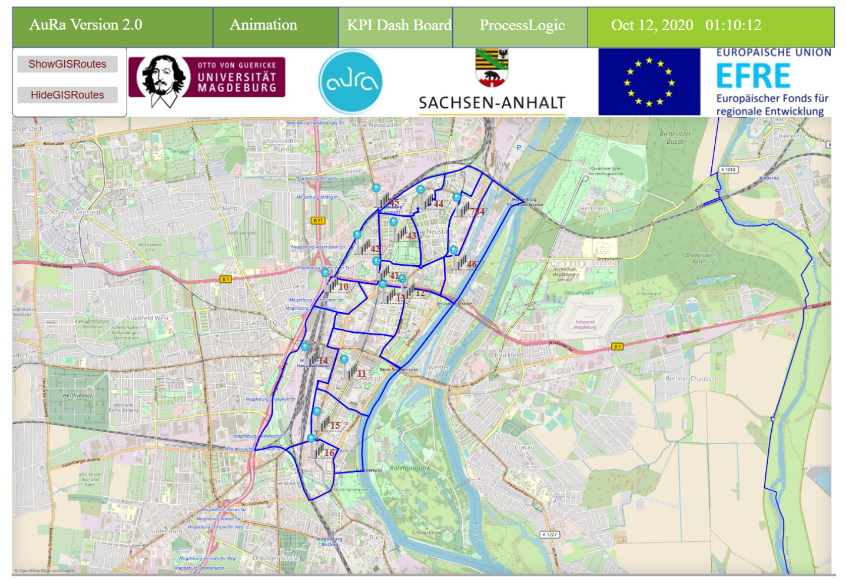
Anylogic provides an inbuilt Geographic Information System (GIS) map. We created the regions on the top layer of the GIS map using a shapefile obtained from Magdeburg’s traffic department. Figure 4 shows the Graphical User Interface (GUI) of the simulation model, which visualizes the operational area, including cargo bikes, stations, and Key Performance Indicator (KPI) dashboard and process logic.

3.3. Fleet Management Strategies

Fleet management is a vital component in the efficiency of OSABS. It defines how bikes are assigned to the customer. We refer to this using the matching problem. It also allows for a redistribution of the bikes in the network to optimize the system. This is called the rebalancing (or relocation) problem. In this paper, we aim to test and evaluate different rebalancing strategies. The matching component will be the subject of further studies. For this work, we implemented a first-in-first-out (FIFO) strategy that assigns the best available bike in the 10-min area (in terms of the less energy-consuming route) to each customer. It is important to mention that we prioritize serving the current requests in the rebalancing operation. This means that, if a bike is on its way to a waiting station and a request appears in the surroundings, the bike could be assigned to this customer’s request, and the rebalancing operation cancelled. We do not consider open requests. If no available bike can reach the customer in less than 10 min, then the request is rejected.

For the rebalancing component, we distinguish between two types of relocation:

• Relocation after rental: refers to the rebalancing operation applied when a bike becomes idle after serving a customer.
• Periodic relocation: refers to the rebalancing operation which occurs each period T to distribute bikes between the different stations according to future demand.

Both types require the implementation of the following steps:

• Stations distribution: We need to discretize the operating area into a set of rebalancing regions (cells) and locate a station in each region. In this work, we adopt the same discretization of statistical cells, for two reasons. First, because the demand scenarios are defined according to the statistical cells. The second reason is that each statistical cell can be covered in 10 min if we place a station in its center. Therefore, we have placed 14 stations (a station in the center of each region).
• Demand estimation: Predicting upcoming demand has been recognized as an important task [57]. However, as we aim to test different relocation strategies and are not interested in evaluating or developing novel forecasting methods, we assume that we know the mean of the demand distribution (generated according to poisson distribution). This assumption has no impact on our comparison study.
• Imbalance calculation: For each relocation type, we have a specific imbalance calculation.
  The imbalance for periodic relocation: For each region i, at the period T, we define the periodic imbalance $P{I}_i\left(T\right)$ according to Equation (1).

  $$P{I}_i\left(T\right)=N_i\left(T\right)-D_i\left(T\right)$$

  (1)

  where:
  • $N_i\left(T\right)$: Number of bikes at the beginning of the period T in the cell i.
  • $D_i\left(T\right)$: Estimated number of bikes needed for the current period in the region i.
  The imbalance for relocation after rental: For each region i, and for each period T, we calculate the imbalance according to the Equation (2).

  $$P_i\left(t\right)=N_i\left(t\right)-D_i\left(t\right)$$

  (2)

  where:
  • For each period T, T <= t < T + 1
  • $N_i\left(t\right)$: Number of bikes available at t in the region i. This value is updated each time a bike from the region i is assigned to a customer (We decrease the value by 1) or a bike is relocated to the station of region i (we increase the value by 1).
  • $D_i\left(t\right)$: Estimated number of bikes needed at t till the end of the current period T. The value of $D_i\left(t\right)$ is updated continuously (it decreases when requests are appearing).
• Bike relocation: we assign each idle bike to a station using imbalance calculation. We have defined three different rebalancing strategies and one reference case where no rebalancing strategy is applied:
  • No Relocation: this is the case where less idle mileage is traveled, where we do not consider the future demand. For the periodic relocation, no action is needed. However, for the relocation after rental, we move the bike to the waiting station of the customer destination region (bikes need to always be in a waiting station).
  • Relocation in the vicinity: for this strategy, bikes can move only to neighboring regions. For the periodic relocation, we relocate bikes from a region with oversupply to undersupplied regions in its vicinity only. The priority is given to the region with the highest deficit in the neighborhood. For relocation after rental, the bike should stay in the customer destination region if it has already a negative imbalance; otherwise, it moves to the region with the highest deficit in the vicinity, If no region has a deficit, the bike is assigned to the waiting station of the destination region.
  • Relocate to any undersupplied cell: in this case, we mainly relocate bikes based on the imbalance value. Each region with an undersupply can get bikes from any region with an oversupply (even if it is distant). However, this operation is optimized by selecting the nearest available bike to the undersupplied region. After the rental, the bike should stay in the customer destination region if it has already a negative imbalance. Otherwise, it goes to the region with the biggest deficit.
  • Mixed relocation: here, we combine the strategies “Relocation in the vicinity” and “relocation to any”. For cells with a significant undersupply (imbalance ≥ 5), relocation is possible from any cell. However, for cells with a moderate undersupply (imbalance < 5), only relocation from neighboring cells is allowed.

In total, we can create 16 scenarios from the combination of these rebalancing strategies. In this first study, we are interested in evaluating the following scenarios: no relocation, relocation to vicinity, relocation to any and mixed relocation. We apply the same strategy for both periodic relocation and relocation after rental.

4. Case Study Results

4.1. Simulation Settings

In order to evaluate the different rebalancing strategies within OSABS, we use the agent-based simulation model developed in the Anylogic Professional 8.6 version. The operational area of OSABS is defined as the 14 regions of Magdeburg (Germany), which constitute the city core (see Figure 4). We run the experiments using a computer Intel (R) i9 CPU @2.40 GHz with 32.0 GB of RAM. The fleet size was initially determined so that we serve, on average, 94% of requests during rhw peak hour in the case where the no-rebalancing strategy is applied. The bikes are initially distributed over the network according to the distribution of demand between the regions. The periodic rebalancing is carried out every hour.

We evaluate OSABS through the following set of indicators:

• Global service level: percentage of served requests.
• Service level during peak hours: the service level in the evening peak (between 18 h and 19 h).
• Empty vehicle mileage Traveled (VMT) for relocation: total mileage driven to redistribute bikes (for relocation purposes) in km.
• Empty mileage Traveled for relocation per bike in km.
• Energy consumption for relocation: the energy consumed for relocation operation in kWh.
• Energy consumption for relocation per bike in kWh.

The generation of requests in Anylogic is stochastic and follows an exponential distributed interarrival time with a mean = 1/arrival rate. Thus, multiple simulation runs are required to guarantee a stable estimation for the average values of our KPIs. The minimum number of required runs of $MNR\left(n\right)$ was calculated for the standard deviation $s\left(n\right)$ of the decisive KPI, as described in Equation (3), based on n initial simulation runs [58] :

$$MNR\left(n\right)=\lceil {(\frac{s\left(n\right)\ast t_{n-1,1-\alpha /2}}{\overline{x}\ast ϵ})}^2\rceil$$

(3)

where:

• $\overline{x}$ is the sample mean.
• $ϵ$ allowable percentage error of the estimate.
• t is the inverse of Student’s t CDF evaluated at $1-\alpha /2$ with $n-1$ degrees of freedom.
• $\alpha$ is the level of significance.

In all cases, the service level is the decisive KPI. Based on $n=10$, $\alpha$ = 0.1 and $ϵ$ = 0.1, MNR is between 6 to 10 runs per scenario. For the following tests, we perform 10 runs per scenario.

Initially, we simulate 24 h (a typical statistical day) for the three relocation strategies and calculate the average number of periodic rebalancing operations. We conclude that nearly 90% of requests and 90% of relocation actions occur between 06:00 a.m. and 09:00 p.m. (Figure 5). As the simulation is time-consuming and multiple runs are required per scenario, we limited the test runs between 06:00 a.m. and 09:00 p.m.

Finally, by analysing the hourly distribution of bookings for each day of the week, we can see that there are two main different demand patters (Figure 6): one for the working days (from Monday to Friday) and one for the weekend (Saturday, Sunday). Consequently, we will conduct our experiments on Wednesday, where there is the highest demand in the evening peak hour, and Saturday.

4.2. Simulation Results

4.2.1. Simulation of Working Day

As the main KPI is the service level, we evaluate the average hourly service level for the different strategies (Figure 7).

As we can see in Figure 7, the average service level for the reference case and the three relocation strategies is higher in the morning peak than in the evening peak. This is an expected outcome, as the demand per hour is highest in the evening peak for our simulated day. We can also observe that the different proactive rebalancing strategies outperform the “No rebalancing” case in the phase of the morning peak (between 07:00 a.m. and 09:00 a.m.). While the service level for the “No rebalancing” strategy decreases from 7:00 a.m., it remains at 100% for the three other strategies till 8 a.m. This is an indicator that bike rebalancing is particularly valuable when low-demand phases are followed by high-demand phases. We also notice the importance of relocation in the abate phase (From 10:00 a.m. to 05:00 p.m.). The service level of the “no rebalancing” case keeps decreasing, while the service level for the proactive relocation strategies increases. The relocation operation allows for the convenient redistribution of bikes after a high-demand phase, consequently achieving demand satisfaction in the different regions. The three relocation strategies achieve comparable service level results during the different hours of the day.

The outcome for the rest of the KPIs for the different scenarios is presented in terms of average values in

Table 2. Average KPIs for the different rebalancing strategies.

Relocation Strategy	Relocation VMT (km)	Relocation VMT per Bike (km)	Relocation Energy (kWh)	Relocation Energy per Bike (kWh)
No rebalancing	3100.785	28.189	107.154	0.974
To vicinity	4736.338	43.058	155.249	1.411
To any	5736.59	52.151	176.198	1.602
Mixed rebalancing	5474.413	49.767	173.315	1.576

.

As expected, the no-rebalancing case outperforms the proactive relocation strategies in terms of energy consumption and mileage traveled. When we do not relocate idle bikes, at least 14 km per bike could be saved, which corresponds to about 0.5 kWh for the simulated scenarios. Among the proactive rebalancing strategies, the “to vicinity” strategy allows the best results to be achieved, since shorter and fewer trips are performed when we relocate bikes only to the neighboring regions. The worst KPI outcomes are obtained by the “to any” strategy, which is the result of excessively spatially distributing the bikes.

As we can see in Figure 7, the initial fleet is oversized, especially for the rebalancing strategies, as about 98% of requests are fulfilled during peak hours. Thus, we also tested the four scenarios for different fleet sizes in order to determine the minimum number of bikes required for each relocation strategy. The variation in global service level and service level during peak hours are correspondingly presented in Figure 8 and Figure 9.

As a first summary of the results, we observe that the three proactive relocation strategies allow for a reduction in the fleet size to only 90 bikes, while serving 94% of the demand during peak hours, with a decrease of about 15% compared to the no-rebalancing strategy (about 105 bikes are needed). This reduction is very valuable, especially when the fleet is a huge investment, as in our case. We also notice that the three strategies have the same performance in terms of service level, and this can also be confirmed by the hourly service level, with 90 bikes (Figure 10).

This decrease in the number of bikes comes with a trade-off. For a large fleet, the bikes are abundant and there is less need to redistribute them; even when a rebalancing is needed, the trips are habitually short. However, when the fleet size is small, bikes need to rebalance often and, thus, a slight increase occurs in the rebalancing mileage traveled per bike (Figure 11) and the energy consumed for rebalancing per bike (Figure 12). However, for the total mileage traveled and energy consumption, we notice a slight decrease when the fleet size is reduced (Figure 13 and Figure 14). With the “to-vicinity” strategy, the total energy consumed for rebalancing is equal to 135,475 kWh. This corresponds to an increase of about 30 kWh compared to the energy consumed with the “no-rebalancing” strategy, to achieve a 94% service level with 105 bikes. Unsurprisingly, the “to-any” strategy performs the worst in terms of resource use. It leads to an increase of about 28% in the mileage traveled and 18% in energy consumption compared to the “to-vicinity” strategy. The performance of the “mixed” strategy is always in between the two other proactive relocation strategies.

4.2.2. Weekend Simulation

We simulated our system for Saturday, with different fleet sizes. As we can see in Figure 15, the minimum fleet size required for the “No rebalancing” case is around 95 bikes. However, we can reduce the fleet to less than 75 bikes if we apply a relocation strategy, while ensuring a service level above 94%.

However, there was an increase in the mileage traveled and the energy consumption when opting for rebalancing (Figure 16 and Figure 17). The most efficient proactive relocation strategy is, as expected, the “To vicinity” strategy. On average, it consumes 14% less energy compared to the “To any” strategy and 11% less compared to the “mixed” relocation. We can also observe that the total mileage traveled and energy consumption significantly decreased for all strategies when the fleet size decreases. With 75 bikes, the rebalancing operation consumes only 107 kWh, on average, when applying the “To vicinity” strategy. However, for the “No rebalancing” case, our system needs 95 bikes and consumes around 90 kWh for the same service level. There is an obvious trade-off between the fleet size reduction (by implementing a rebalancing strategy) and the energy consumption reduction (by avoiding relocation operations).

The mileage traveled per bike and the energy consumed per bike are nearly constant, even when decreasing the fleet size for the different strategies, as shown in

Table 3. Average mileage traveled per bike for the different rebalancing strategies with different fleet sizes (in km).

Relocation Strategy	95 Bikes	90 Bikes	85 Bikes	80 Bikes	75 Bikes
No rebalancing	27.2	26.74	28.24	28.41	28.76
To vicinity	43.52	44.2	44.53	45.43	43.98
To any	56.16	55.17	55.18	55.01	52.93
Mixed rebalancing	52.34	51.82	53	51.26	51.14

and

Table 4. Average energy consumption per bike for the different rebalancing strategies with different fleet sizes (in kWh).

Relocation Strategy	95 Bikes	90 Bikes	85 Bikes	80 Bikes	75 Bikes
No rebalancing	0.94	0.93	0.98	0.99	1
To vicinity	1.42	1.44	1.45	1.47	1.43
To any	1.7	1.68	1.69	1.68	1.62
Mixed rebalancing	1.62	1.61	1.65	1.6	1.6

. In this scenario, the mileage traveled per bike increases by at least 14 km, on average, when applying a rebalancing strategy. We also found approximately the same difference in the energy consumption as the workday scenario (about 500 Wh between the “no rebalancing” case and the “to vicinity” strategy).

4.3. Cost Analysis

Several papers in the literature have defined the operational cost of AMoD services and evaluated the fleet management strategies accordingly [2,37,59]. Introducing financial indicators such as energy cost, cost of a lost request, and bicycle depreciation value allows for a better comparison between the different strategies and helps stakeholders more easily make a decision. In our case, we ignored the cost of a lost request but we considered the service level when comparing the different strategies. As we are studying a novel system, which is still under development, complete and exact data on costs are not available at present. However, based on talks with industry experts and our best knowledge of the current market prices, we assume the list of costs given in

Table 5. Bike and charging station cost assumptions.

	Bike Capital	Bike Maintenance	Charging Station Implementation	Charging Station Maintenance	Electricity (per kWh)
Costs in €	30,000 €	300 €/month	45,000 €	150 €/month	0.3 €/kWh
Costs per hour in €	0.856 €	0.417 €	0.514 €	0.208 €

. The charging station cost corresponds to a station with five chargers. The cost of a waiting station is ignored because there no infrastructure is needed for its implementation. We also calculate the cost per hour for the different fixed costs, based on a depreciation value of 10 years for the charging station and 4 years for our bike. As the bike is equipped with expensive technology and cameras that protect it from theft and violence, we estimate a higher lifespan than the actual one for electric bikes (generally between 1 and two years [60,61]).

We calculate the energy consumption costs and the total fixed costs for the four different rebalancing cases (

Table 6. Fixed and variable costs for the different rebalancing options.

Rebalancing Strategy	In-Use Energy Consumption in kWh	Idle Energy Consumption in kWh	Energy Consumption Costs	Fleet Size	Fixed Costs
No rebalancing	412.553	479.668	267.667 €	105	2113.014 €
To vicinity	464.963	349.095	244.217 €	90	2070.844 €
To any	522.414	338.20	258.184 €	90	2084.811 €
Mixed	497.808	342.937	252.223 €	90	2078.85 €

). The different values are for our 15-h simulation. For the no-rebalancing case, we use the values obtained for a fleet size of 105 bikes, because this is the required fleet size to achieve a service level of 94%, while the required size is 90 bikes for the three proactive rebalancing strategies. We differentiate between the two types of energy consumption. The first one is the energy consumed when the bike is in use in either the manual mode (when the customer is driving) or by the autonomous mode (for rebalancing purposes or when the bike is driving to a customer). The second type is the energy consumed when the bike is idle (our bike also consumes energy when it is idle because it has sensors and cameras and should always be connected to a server). The second type increases when the bike usage decreases, as is the case when no rebalancing strategy is implemented. Following our first study, we concluded that we need 10 charging stations for our current implementation.

Finally, we can conclude the total costs and a cost per trip (

Table 7. Total costs for the different rebalancing options.

Rebalancing Strategy	Total Costs	Number of Satisfied Trips	Cost per Trip
No rebalancing	2380.681 €	8072	0.295 €
To vicinity	2070.844 €	8017	0.258 €
To any	2084.811 €	8014	0.260 €
Mixed	2078.85 €	8013	0.259 €

).

As we can see, the “To vicinity” strategy has the lowest cost per trip. The difference between the three proactive strategies is very minimal. However, we can notice an important difference between the “no rebalancing” case and the rest of the strategies. This confirms the importance of fleet reduction in order to minimize costs. Indeed, as our bike constitutes a huge investment, opting for a relocation strategy that allows for fleet reduction and the efficient use of resources can be the best choice for stakeholders. It is important to highlight that our cost per trip does not include costs such as marketing, insurance, website hosting, and administrative costs. These costs are hard to estimate before implementing OSABS. For this reason, we can not compare the cost per trip of our system to the conventional bike-sharing system, where only the operative cost per trip was estimated as 0.6 € for the traditional bike-sharing system and 1.06 € for the electrical bike-sharing system [60]. Instead, we can compare the cost of rebalancing based on the data given in [60] for the traditional bike-sharing and the electrical bike-sharing.

Table 8. Comparison of rebalancing costs of different bike-sharing systems.

Bike-Sharing System	Rebalancing Costs per Hour and Bike
OSABS	0.03 €/h-bike
Traditional	0.028 €/h-bike
Electrical	0.09 €/h-bike

states the rebalancing cost of our “to vicinity” strategy and other bike-sharing systems.

As we can see, OSABS rebalancing costs can be compared to the conventional system. Our costs are slightly higher than traditional bike-sharing but we can also estimate higher revenues, because we intend to have additional revenue channels to cover the cost difference. Compared to the electrical bike-sharing systems, we can see that OSABS performs better in terms of relocation costs.

5. Discussion

In this section, we discuss the presented outcomes and outline their limitations. First, this paper presents an approach to implement and compare different relocation strategies for AMoD services. This approach could easily be applied to other types of mobility where a proactive rebalancing operation is needed.

Second, it is important to analyze the simulation results with a holistic view of the different associated factors. Evidently, for fixed fleet size, the rebalancing operation leads to higher empty mileage traveled (and, consequently, higher energy consumption) in the system. However, as shown in the evaluation results, rebalancing allows us to significantly lower the number of bikes in the system (by over 15% for the same service level). The decrease in fleet size implies significant financial benefits thanks to the lower investments, maintenance costs and energy consumption. The amount of energy saved needs to be determined by life-cycle assessment in future work. These benefits might be even larger when we also consider the environmental advantages. A smaller fleet results in less street congestion and fewer parking spaces for waiting and charging stations.

Third, we believe that the cost analysis is not conclusive, as the costs may differ considerably from one city to another [62] and strictly depend on the implemented system, the area, and the demand profiles [63]. To the best of our knowledge, data for German cities are, unfortunately, not available in the literature. For OSABS, we estimate high operational costs compared to the conventional system. However, it can confer additional benefits by modifying the user’s behavior and enhancing the attractiveness of bike-sharing. As mentioned in [63], we could have different bike-sharing systems in the same area for different target groups and with different business models. For example, the electrical bike-sharing system costs more than the traditional bike-sharing but makes the bike-sharing more attractive, and the increase in infrastructure could be compensated by a larger and more balanced demand [60]. The same applies to OSABS, which is estimated to attract more users thanks to the system reactivity and the possibility of a door-to-door bike-sharing option. Indeed, OSABS not only can be considered as an alternative to cars for short trips but also can enhance the transition from cars to public transportation for mid-to-long trips. It facilitates the connection to public transport stations and can be used as a first- or last-mile mobility option. Furthermore, it would be worth comparing OSABS and AMoD services in terms of their external costs. As, for instance, Cavill et al. [64], Gössling and Choi [65], Koning and Conway [66] point out, biking benefits an economy or society through better health and other factors. Cars, however, impose costs on a society through air pollution, health issues and accidents. Although OSABS may not be viable from an operator perspective, they are likely to beneficial from a public perspective. However, this needs more investigation and sound assessments of the external costs of OSABS and AMoDs.

Fourth, we should highlight that we ran the experiments for only two demand scenarios in the inner city of Magdeburg. Thus, the results must be interpreted considering the context of the study area and the demand patterns. We simulated the system for a dense and small area, where the bike can move from one region to another in 2–3 min and the demand is mainly concentrated in the central region. In this setting, the relocation to a vicinity strategy has proven to be the most efficient in terms of service level and energy consumption. However, if we consider a larger area, where we have distant clusters of demand, a different strategy could perform better. For example, including the outer city areas in our study would stress the importance of rebalancing to meet customer demands in the suburbs. Indeed, in the morning peak hour, the demand is in the inner city, where we will have a lot of bikes; however, if we need more bikes in the outer city, there is no supply. In this case, the rebalancing “To vicinity” may lead to poor performances as the outer city is distant from the inner-city regions, and thus cannot follow the demand pattern. However, the strategy “To any” and “mixed” may perform better and ensure a good service level. Certainly, the rebalancing distance will increase, but we will satisfy more customers and the manual km (the kilometers driven by the customer, which is a source of revenue for our service) will also increase. A dynamic pricing strategy could be tested and studied for this scenario, in which we propose a higher price for the outer regions, as we need a larger rebalancing effort to satisfy demand. This case also emphasizes the need for OSABS, as bikes can move autonomously and dynamically according to the upcoming demand, unlike conventional bike-sharing systems, which are currently not viable for such regions. The evaluation of relocation strategies with different cities and case studies will be the subject of future research.

Fifth, in this work, we ignored the need for the bikes to charge their batteries. As has been studied by Chen et al. [36], the choice of the charging policy and vehicle range has a major impact on the system performance. Thus, an advanced model with battery and charging integration is under development. The next work will aim to optimize charging and fleet management jointly.

Finally, the demand information used in the rebalancing algorithm is the same as the one integrated into the demand generation module, which is not the case in the real world. A sophisticated forecasting algorithm for rebalancing should be implemented and tested in order to present a more realistic model. A deep learning-based approach could be used to predict demand location and time [67], and the rebalancing algorithm assigns bikes accordingly. Further work could also be done to optimize rebalancing by forecasting the customer destination.

6. Conclusions

Through this work, we investigate and provide a better knowledge of a novel mobility service: OSABS. We address the problem of fleet relocation. Our aim is to optimize fleet management for this new service by increasing its efficiency and reducing investment costs, which are relatively high for a self-driving system. The simulation of our case study with three different strategies for periodic rebalancing and after rental rebalancing allows us to quantify the impact of each one on the service level and in terms of resource use, compared to a reference case of “no rebalancing”. Among the three proactive rebalancing strategies, redistributing bikes within the vicinity of the current region achieves the best performance, with low energy consumption, low mileage traveled, and a high service level. In contrast, strategies aiming to relocate bikes more often lead to lower performances in terms of the resources used, with no advantage in the service level. These findings were also strengthened by the cost analysis, where the “to vicinity” strategy achieved the smallest cost per trip for a given service level.

This study affirms the rebalancing’s potential in the improvement of service efficiency and reduction in fleet size. In addition, it contributes to the field of SAV fleet management research by extending the scope of existing studies to other mobility services, such as autonomous bikes or micro-vehicles, with more realism. This study allowed us to draw some conclusions for OSABS regarding the most suitable rebalancing strategy. However, the simulated model is very simplified and could be extended further. We can add more complexity by considering in-advance booking, a heterogeneous fleet, or dynamic prices. Furthermore, in this research, we considered OSABS independently from other mobility services. With this limitation, we miss the potential gains that may arise through integrating our service with public transportation. A future research direction consists of the evaluation of OSABS for more complex deployment options, such as a multi-modal transportation service or a last-mile solution.

References

1. Dandl, F.; Bogenberger, K. Comparing Future Autonomous Electric Taxis with an Existing Free-Floating Carsharing System. IEEE Trans. Intell. Transp. Syst. 2019, 20, 2037–2047. [Google Scholar] [CrossRef]
2. Zhang, R.; Spieser, K.; Frazzoli, E.; Pavone, M. Models, algorithms, and evaluation for autonomous mobility-on-demand systems. In Proceedings of the 2015 American Control Conference (ACC), Chicago, IL, USA, 1–3 July 2015; pp. 2573–2587. [Google Scholar] [CrossRef]
3. Fraedrich, E.; Kröger, L.; Bahamonde-Birke, F.; Frenzel, I.; Liedtke, G.; Trommer, S.; Lenz, B.; Heinrichs, D. Automatisiertes Fahren im Personen- und Güterverkehr; e-mobil BW GmbH; Deutsches Zentrum für Luft- und Raumfahrt e.V. Institut für Verkehrsforschung; Ministerium für Verkehr Baden-Württemberg: Berlin, Germany, 2017. [Google Scholar]
4. Hörl, S.; Becker, F.; Dubernet, T.; Axhausen, K.W. Induzierter Verkehr durch autonome Fahrzeuge: Eine Abschätzung; Eidgenössisches Departement für Umwelt, Verkehr, Energie und Kommunikation (UVEK); Bundesamt für Strassen (ASTRA): Zurich, Switzerland, 2019. [Google Scholar]
5. Millard-Ball, A. Pedestrians, Autonomous Vehicles, and Cities. J. Plan. Educ. Res. 2018, 38, 6–12. [Google Scholar] [CrossRef]
6. Gehl, J. Cities for People; Island Press: Washington, DC, USA, 2010. [Google Scholar]
7. Pozoukidou, G.; Chatziyiannaki, Z. 15-Minute City: Decomposing the New Urban Planning Eutopia. Sustainability 2021, 13, 928. [Google Scholar] [CrossRef]
8. Nations, U. New Urban Agenda; Habital 3: Quito, Ecuador, 2017. [Google Scholar]
9. Assmann, T.; Matthies, E.; Gehlmann, F.; Schmidt, S. Shared autonomous cargo bike fleets-a better solution for future mobility than shared autonomous car fleets? In Proceedings of the European Transport Conference 2020, Online, 9–11 September 2020. [Google Scholar]
10. Becker, S.; Rudolf, C. Exploring the potential of free cargo-bikesharing for sustainable mobility. GAIA 2018, 27, 156–164. [Google Scholar] [CrossRef]
11. Hess, A.K.; Schubert, I. Functional perceptions, barriers, and demographics concerning e-cargo bike sharing in Switzerland. Transp. Res. Part D Transp. Environ. 2019, 71, 153–168. [Google Scholar] [CrossRef]
12. Clausen, U.; Stütz, S.; Bernsmann, A.; Heinrichmeyer, H. ZF-ZUKUNFTSSTUDIE 2016 Die letzte Meile; ZF Friedrichshafen AG: Friedrichshafen, Germany, 2016. [Google Scholar]
13. Baum, L.; Assmann, T.; Strubelt, H. State of the art - Automated micro-vehicles for urban logistics. IFAC-PapersOnLine 2019, 52, 2455–2462. [Google Scholar] [CrossRef]
14. Schmidt, S.; Assmann, T.; Junge, L.; Höfer, M.; Krause, K.; Manoeva, D.; Matthies, E.; Meißner, S.; Petersen, H.; Riestock, M.; et al. Shared autonomous cargo bike fleets—Approaches for a novel sustainable urban mobility solution. In Proceedings of the Fisita World Congress 2021, Online, 14–16 September 2021. [Google Scholar]
15. Clemente, M.; Fanti, M.P.; Mangini, A.; Ukovich, W. The Vehicle Relocation Problem in Car Sharing Systems: Modeling and Simulation in a Petri Net Framework. In International Conference on Applications and Theory of Petri Nets and Concurrency; Springer: Berlin/Heidelberg, Germany, 2013; Volume 7927, pp. 250–269. [Google Scholar] [CrossRef]
16. Haider, Z.; Charkhgard, H.; Kim, S.W.; Kwon, C. Optimizing the Relocation Operations of Free-Floating Electric Vehicle Sharing Systems. SSRN Electron. J. 2019. [Google Scholar] [CrossRef]
17. Illgen, S.; Höck, M. Literature review of the vehicle relocation problem in one-way car sharing networks. Transp. Res. Part B Methodol. 2019, 120, 193–204. [Google Scholar] [CrossRef]
18. Dell’Amico, M.; Hadjicostantinou, E.; Iori, M.; Novellani, S. The bike sharing rebalancing problem: Mathematical formulations and benchmark instances. Omega 2014, 45, 7–19. [Google Scholar] [CrossRef]
19. Dell’Amico, M.; Iori, M.; Novellani, S.; Subramanian, A. The Bike sharing Rebalancing Problem with Stochastic Demands. Transp. Res. Part B Methodol. 2018, 118, 362–380. [Google Scholar] [CrossRef]
20. Winter, K.; Cats, O.; Arem, B.V.; Martens, K. Impact of relocation strategies for a fleet of shared automated vehicles on service efficiency, effectiveness and externalities. In Proceedings of the 2017 5th IEEE International Conference on Models and Technologies for Intelligent Transportation Systems (MT-ITS), Naples, Italy, 26–28 June 2017; pp. 844–849. [Google Scholar] [CrossRef]
21. Winter, K.; Cats, O.; Martens, K.; van Arem, B. Relocating shared automated vehicles under parking constraints: Assessing the impact of different strategies for on-street parking. Transportation 2020, 48, 1931–1965. [Google Scholar] [CrossRef]
22. Schmid, V. Solving the dynamic ambulance relocation and dispatching problem using approximate dynamic programming. Eur. J. Oper. Res. 2012, 219, 611–621. [Google Scholar] [CrossRef] [Green Version]
23. Brotcorne, L.; Laporte, G.; Semet, F. Ambulance location and relocation models. Eur. J. Oper. Res. 2003, 147, 451–463. [Google Scholar] [CrossRef]
24. Saint-Guillain, M.; Paquay, C.; Limbourg, S. Time-dependent stochastic vehicle routing problem with random requests: Application to online police patrol management in Brussels. Eur. J. Oper. Res. 2021, 292, 869–885. [Google Scholar] [CrossRef]
25. Bélanger, V.; Lanzarone, E.; Ruiz, A.B.; Soriano, P. The Ambulance Relocation and Dispatching Problem; CIRRELT: Montréal, QC, Canada, 2015. [Google Scholar]
26. Pillac, V.; Gendreau, M.; Guéret, C.; Medaglia, A.L. A review of dynamic vehicle routing problems. Eur. J. Oper. Res. 2013, 225, 1–11. [Google Scholar] [CrossRef] [Green Version]
27. Psaraftis, H.N.; Wen, M.; Kontovas, C.A. Dynamic vehicle routing problems: Three decades and counting. Networks 2016, 67, 3–31. [Google Scholar] [CrossRef] [Green Version]
28. Espegren, H.M.; Kristianslund, J.; Andersson, H.; Fagerholt, K. The Static Bicycle Repositioning Problem—Literature Survey and New Formulation; Springer: Cham, Siwtzerland, 2016; Volume 9855. [Google Scholar] [CrossRef] [Green Version]
29. Daskin, M. A Maximum Expected Covering Location Model: Formulation, Properties and Heuristic Solution. Transp. Sci. 1983, 17, 48–70. [Google Scholar] [CrossRef] [Green Version]
30. Gendreau, M.; Laporte, G.; Semet, F. A dynamic model and parallel tabu search heuristic for real-time ambulance relocation. Parallel Comput. 2001, 27, 1641–1653. [Google Scholar] [CrossRef] [Green Version]
31. Chiariotti, F.; Pielli, C.; Zanella, A.; Zorzi, M. A dynamic approach to rebalancing bike-sharing systems. Sensors 2018, 18, 512. [Google Scholar] [CrossRef] [Green Version]
32. Hyland, M.F.; Mahmassani, H.S. Taxonomy of shared autonomous vehicle fleet management problems to inform future transportation mobility. Transp. Res. Rec. 2017, 2653, 26–34. [Google Scholar] [CrossRef]
33. Narayanan, S.; Chaniotakis, E.; Antoniou, C. Shared autonomous vehicle services: A comprehensive review. Transp. Res. Part C Emerg. Technol. 2020, 111, 255–293. [Google Scholar] [CrossRef]
34. Weikl, S.; Bogenberger, K. Relocation strategies and algorithms for free-floating car sharing systems. IEEE Intell. Transp. Syst. Mag. 2013, 5, 100–111. [Google Scholar] [CrossRef]
35. Fagnant, D.J.; Kockelman, K.M. The travel and environmental implications of shared autonomous vehicles, using agent-based model scenarios. Transp. Res. Part C Emerg. Technol. 2014, 40, 1–13. [Google Scholar] [CrossRef]
36. Chen, T.D.; Kockelman, K.M.; Hanna, J.P. Operations of a shared, autonomous, electric vehicle fleet: Implications of vehicle and charging infrastructure decisions. Transp. Res. Part A Policy Pract. 2016, 94, 243–254. [Google Scholar] [CrossRef] [Green Version]
37. Spieser, K.; Samaranayake, S.; Gruel, W.; Frazzoli, E. Shared-Vehicle Mobility-on-Demand Systems: A Fleet Operator’s Guide to Rebalancing Empty Vehicles. In Proceedings of the Transportation Research Board 95th Annual Meeting, Washington, DC, USA, 10–14 January 2016. [Google Scholar]
38. Pavone, M.; Smith, S.L.; Frazzoli, E.; Rus, D. Robotic load balancing for mobility-on-demand systems. Int. J. Robot. Res. 2012, 31, 839–854. [Google Scholar] [CrossRef]
39. Tsao, M.; Iglesias, R.; Pavone, M. Stochastic Model Predictive Control for Autonomous Mobility on Demand. In Proceedings of the 2018 21st International Conference on Intelligent Transportation Systems (ITSC), Maui, HI, USA, 4–7 November 2018; pp. 3941–3948. [Google Scholar] [CrossRef] [Green Version]
40. Azevedo, C.L.; Marczuk, K.; Raveau, S.; Soh, H.; Adnan, M.; Basak, K.; Loganathan, H.; Deshmunkh, N.; Lee, D.H.; Frazzoli, E.; et al. Microsimulation of demand and supply of autonomous mobility on demand. Transp. Res. Rec. 2016, 2564, 21–30. [Google Scholar] [CrossRef]
41. Wallar, A.; Zee, M.V.D.; Alonso-Mora, J.; Rus, D. Vehicle Rebalancing for Mobility-on-Demand Systems with Ride-Sharing. In Proceedings of the 2018 IEEE/RSJ International Conference on Intelligent Robots and Systems (IROS), Madrid, Spain, 1–5 October 2018; pp. 4539–4546. [Google Scholar] [CrossRef] [Green Version]
42. Marczuk, K.A.; Soh, H.S.; Azevedo, C.M.; Lee, D.H.; Frazzoli, E. Simulation Framework for Rebalancing of Autonomous Mobility on Demand Systems; EDP Sciences: Les Ulis, France, 2016; Volume 81. [Google Scholar] [CrossRef] [Green Version]
43. Brendel, A.B.; Lichtenberg, S.; Nastjuk, I.; Kolbe, L.M. Adapting Carsharing Vehicle Relocation Strategies for Shared Autonomous Electric Vehicle Services; ICIS: Seoul, Korea, 2017. [Google Scholar]
44. Cantelmo, G.; Kucharski, R.; Antoniou, C. Low-Dimensional Model for Bike-Sharing Demand Forecasting that Explicitly Accounts for Weather Data. Transp. Res. Rec. 2020, 2674, 132–144. [Google Scholar] [CrossRef]
45. Giot, R.; Cherrier, R. Predicting bikeshare system usage up to one day ahead. In Proceedings of the IEEE SSCI 2014: 2014 IEEE Symposium Series on Computational Intelligence—CIVTS 2014: 2014 IEEE Symposium on Computational Intelligence in Vehicles and Transportation Systems, Proceedings, Orlando, FL, USA, 9–12 December 2014; pp. 22–29. [Google Scholar] [CrossRef] [Green Version]
46. Chen, L.; Zhang, D.; Wang, L.; Yang, D.; Ma, X.; Li, S.; Wu, Z.; Pan, G.; Nguyen, T.M.T.; Jakubowicz, J. Dynamic cluster-based over-demand prediction in bike sharing systems. In Proceedings of the UbiComp 2016 ACM International Joint Conference on Pervasive and Ubiquitous Computing, Heidelberg, Germany, 12–16 September 2016; pp. 841–852. [Google Scholar] [CrossRef]
47. Yang, Z.; Hu, J.; Shu, Y.; Cheng, P.; Chen, J.; Moscibroda, T. Mobility modeling and prediction in bike-sharing systems. In Proceedings of the MobiSys 2016—Proceedings of the 14th Annual International Conference on Mobile Systems, Applications, and Services, Singapore, 26–30 June 2016; pp. 165–178. [Google Scholar] [CrossRef]
48. Lin, L.; He, Z.; Peeta, S. Predicting station-level hourly demand in a large-scale bike-sharing network: A graph convolutional neural network approach. Transp. Res. Part C Emerg. Technol. 2018, 97, 258–276. [Google Scholar] [CrossRef] [Green Version]
49. Frade, I.; Ribeiro, A. Bicycle Sharing Systems Demand. Procedia Soc. Behav. Sci. 2014, 111, 518–527. [Google Scholar] [CrossRef] [Green Version]
50. Garcia-Gutierrez, J.; Romero-Torres, J.; Gaytan-Iniestra, J. Dimensioning of a Bike Sharing System (BSS): A Study Case in Nezahualcoyotl, Mexico. Procedia Soc. Behav. Sci. 2014, 162, 253–262. [Google Scholar] [CrossRef] [Green Version]
51. Steierwald, G.; Künne, H.D.; Vogt, W. (Eds.) Stadtverkehrsplanung; Springer: Berlin/Heidelberg, Germany, 2005. [Google Scholar] [CrossRef]
52. Call a Bike—Buchungen Call a Bike (Stand 05/2017)—Open-Data-Portal—Deutsche Bahn Datenportal ABN. Available online: https://data.deutschebahn.com/dataset/data-call-a-bike/resource/0fcce4dd-7fc6-43f8-a59c-983a7945f8ba.htmlr (accessed on 7 May 2021).
53. Gebhart, K.; Noland, R.B. The impact of weather conditions on bikeshare trips in Washington, DC. Transportation 2014, 41, 1205–1225. [Google Scholar] [CrossRef]
54. Haj-Salah, I.; Mukku, V.D.; Schmidt, S.; Assmann, T. A Conceptual Model for the Simulation of the Next Generation Bike-Sharing System with Self-driving Cargo-Bikes; Springer: Cham, Switzerland, 2021; Volume 1278, pp. 253–262. [Google Scholar] [CrossRef]
55. Vasu Dev, M.; Imen Haj, S.; Tom, A. Simulation Testbed for the next-generation Bike-Sharing System with Self-driving Cargo-Bikes. In Proceedings of the INCOM 2021, 17th IFAC Symposium on Information Control Problems in Manufacturing, Budapest, Hungary, 7–9 June 2021; In press. [Google Scholar]
56. GitHub—Graphhopper/Graphhopper: Open Source Routing Engine for OpenStreetMap. Use It as Java Library or Server. Available online: https://github.com/graphhopper/graphhopper (accessed on 28 May 2021).
57. Brendel, A.; Brauer, B.; Hildebrandt, B. Toward User-Based Relocation Information Systems in Station-Based One-Way Car Sharing. In Proceedings of the AMCIS 2016 Proceedings, San Diego, CA, USA, 11–14 August 2016. [Google Scholar]
58. Truong, L.T.; Sarvi, M.; Currie, G.; Garoni, T.M. How Many Simulation Runs are Required to Achieve Statistically Confident Results: A Case Study of Simulation-Based Surrogate Safety Measures. In Proceedings of the 2015 IEEE 18th International Conference on Intelligent Transportation Systems, Gran Canaria, Spain, 15–18 September 2015; pp. 274–278. [Google Scholar] [CrossRef]
59. Loeb, B.; Kockelman, K.M. Fleet performance and cost evaluation of a shared autonomous electric vehicle (SAEV) fleet: A case study for Austin, Texas. Transp. Res. Part A Policy Pract. 2019, 121, 374–385. [Google Scholar] [CrossRef]
60. Soriguera, F.; Jiménez-Meroño, E. A continuous approximation model for the optimal design of public bike-sharing systems. Sustain. Cities Soc. 2020, 52, 101826. [Google Scholar] [CrossRef]
61. Martinez, L.M.; Caetano, L.; Eiró, T.; Cruz, F. An Optimisation Algorithm to Establish the Location of Stations of a Mixed Fleet Biking System: An Application to the City of Lisbon. Procedia Soc. Behav. Sci. 2012, 54, 513–524. [Google Scholar] [CrossRef] [Green Version]
62. ITDP. The Bikeshare Planning Guide; Institute for Transportation and Development Policy: New York, NY, USA, 2018. [Google Scholar]
63. Audikana, A.; Ravalet, E.; Baranger, V.; Kaufmann, V. Implementing bikesharing systems in small cities: Evidence from the Swiss experience. Transp. Policy 2017, 55, 18–28. [Google Scholar] [CrossRef]
64. Cavill, N.; Kahlmeier, S.; Rutter, H.; Racioppi, F.; Oja, P. Economic analyses of transport infrastructure and policies including health effects related to cycling and walking: A systematic review. Transp. Policy 2008, 15, 291–304. [Google Scholar] [CrossRef]
65. Gössling, S.; Choi, A.S. Transport transitions in Copenhagen: Comparing the cost of cars and bicycles. Ecol. Econ. 2015, 113, 106–113. [Google Scholar] [CrossRef]
66. Koning, M.; Conway, A. The good impacts of biking for goods: Lessons from Paris city. Case Stud. Transp. Policy 2016, 4, 259–268. [Google Scholar] [CrossRef]
67. Kim, S.; Lee, U.; Lee, I.; Kang, N. Idle Vehicle Relocation Strategy through Deep Learning for Shared Autonomous Electric Vehicle System Optimization. arXiv 2020, arXiv:2010.09847. [Google Scholar]
Figure 1. The basic concept of OSABS [9].
Futuretransp 01 00027 g001
Figure 2. Proceeding for the creation of the demand scenario.
Futuretransp 01 00027 g002
Figure 3. Example of the Origin-Destination flows.
Futuretransp 01 00027 g003
Figure 4. Operational area inner-city Magdeburg.
Futuretransp 01 00027 g004
Figure 5. Evolution of demand and rebalancing operations during the day.
Futuretransp 01 00027 g005
Figure 6. Hourly distribution of bookings for a week.
Futuretransp 01 00027 g006
Figure 7. Variation of the service level during the day for 110 bikes.
Futuretransp 01 00027 g007
Figure 8. Variation in the service level according to the fleet size.
Futuretransp 01 00027 g008
Figure 9. Variation in the service level during peak hours according to the fleet size.
Futuretransp 01 00027 g009
Figure 10. Variation of the service level during the day for 90 bikes.
Futuretransp 01 00027 g010
Figure 11. Rebalancing mileage traveled per bike for different fleet sizes.
Futuretransp 01 00027 g011
Figure 12. Energy consumption for rebalancing per bike for different fleet sizes.
Futuretransp 01 00027 g012
Figure 13. Rebalancing mileage traveled for different fleet sizes.
Futuretransp 01 00027 g013
Figure 14. Rebalancing energy consumption for different fleet sizes.
Futuretransp 01 00027 g014
Figure 15. Variation of the service level for different fleet sizes for Saturday.
Futuretransp 01 00027 g015
Figure 16. Rebalancing mileage traveled for different fleet sizes (Saturday).
Futuretransp 01 00027 g016
Figure 17. Rebalancing energy consumption for different fleet sizes (Saturday).
Futuretransp 01 00027 g017