Article

Deep Learning Architectures for Skateboarder–Pedestrian Surrogate Safety Measures

by
Chowdhury Erfan Shourov
1,
Mahasweta Sarkar
1,
Arash Jahangiri
2 and
Christopher Paolini
1,*
1
Department of Electrical and Computer Engineering, San Diego State University, San Diego, CA 92182, USA
2
Department of Civil, Construction and Environmental Engineering, San Diego State University, San Diego, CA 92182, USA
*
Author to whom correspondence should be addressed.
Future Transp. 2021, 1(2), 387-413; https://doi.org/10.3390/futuretransp1020022
Submission received: 28 June 2021 / Revised: 25 August 2021 / Accepted: 9 September 2021 / Published: 12 September 2021

Abstract

:
Skateboarding as a method of transportation has become prevalent, which has increased the occurrence and likelihood of pedestrian–skateboarder collisions and near-collision scenarios in shared-use roadway areas. Collisions between pedestrians and skateboarders can result in significant injury. New approaches are needed to evaluate shared-use areas prone to hazardous pedestrian–skateboarder interactions, and perform real-time, in situ (e.g., on-device) predictions of pedestrian–skateboarder collisions as road conditions vary due to changes in land usage and construction. A mechanism called the Surrogate Safety Measures for skateboarder–pedestrian interaction can be computed to evaluate high-risk conditions on roads and sidewalks using deep learning object detection models. In this paper, we present the first ever skateboarder–pedestrian safety study leveraging deep learning architectures. We view and analyze state of the art deep learning architectures, namely the Faster R-CNN and two variants of the Single Shot Multi-box Detector (SSD) model to select the correct model that best suits two different tasks: automated calculation of Post Encroachment Time (PET) and finding hazardous conflict zones in real-time. We also contribute a new annotated data set that contains skateboarder–pedestrian interactions that has been collected for this study. Both our selected models can detect and classify pedestrians and skateboarders correctly and efficiently. However, due to differences in their architectures and based on the advantages and disadvantages of each model, both models were individually used to perform two different set of tasks. Due to improved accuracy, the Faster R-CNN model was used to automate the calculation of post encroachment time, whereas to determine hazardous regions in real-time, due to its extremely fast inference rate, the Single Shot Multibox MobileNet V1 model was used. An outcome of this work is a model that can be deployed on low-cost, small-footprint mobile and IoT devices at traffic intersections with existing cameras to perform on-device inferencing for in situ Surrogate Safety Measurement (SSM), such as Time-To-Collision (TTC) and Post Encroachment Time (PET). SSM values that exceed a hazard threshold can be published to an Message Queuing Telemetry Transport (MQTT) broker, where messages are received by an intersection traffic signal controller for real-time signal adjustment, thus contributing to state-of-the-art vehicle and pedestrian safety at hazard-prone intersections.

1. Introduction

Skateboarding as means of short distance transportation is attaining wide popularity. The 2020 Summer Olympics in Tokyo, which took place in 2021, featured skateboarding as a competitive sport for the first time [1]. Skateboarders maneuvering in areas with condensed pedestrian traffic elevates the probability of skateboarder–pedestrian collision or near-collision events. Pedestrians walking or standing on sidewalks can also be susceptible and may need to dodge relatively fast moving skateboarders. A widely used mechanism for approximating risks in regions of a roadway shared with multifarious vehicles is termed Surrogate Safety Measures (SSM). These quantifiers provide a probability of near-collision occurrences by calculating the temporal and spatial proximity among road users. Among adolescents aged between 5 and 19 years, skateboarding has been reported to be the most notable cause of injury [2]. Skateboarders travel at a substantially higher velocity relative to the velocity of pedestrians walking on sidewalks and therefore skateboarders are required to conduct maneuvers to avoid colliding with moving and fixed pedestrians and other obstacles. Moreover, skateboarders will often encroach into roadways designated exclusively for vehicular traffic when transitioning between sidewalks. Traumatic injuries can occur when skateboarders collide with vehicles or pedestrians [3].
SSMs are numerical metrics used to pinpoint critical safety related events, such as near collision occurrences, that transpire in particular areas on a thoroughfare. SSM values that exceed a certain hazardous threshold can be used to redesign roadways or justify the adoption of traffic routing policies designed to lower the probability of collisions or near-collision incidents between skateboarders and pedestrians. The conventional approach taken to gauge the safety of thoroughfares with excessive pedestrian density is to accumulate and then later inspect a long history of incident data before enacting design or policy refinements. Skateboarder–pedestrian encounters are rare events, so multiple years of data acquisition are typically needed before changes in policy are enacted. In addition, several recorded incidents between skateboarders and pedestrians are needed to gain the attention of city officials in order for actions be taken to improve safety. Unfortunately, each incident potentially results in trauma or musculoskeletal injury to both skateboarder and pedestrian [4,5]. A reactive approach to safety improvement may be impeded by modifications to roadways and sidewalks due to changes in land use, which impacts long-term safety analysis. Therefore, more proactive approaches are needed to assess thoroughfare safety, ideally in real-time, to decrease the probability of near-collision events. Such approaches can be used to evaluate the safety of skateboarders and pedestrians who utilize areas that may structurally change over time due to construction and other land-use demands. The field of artificial intelligence has excelled over the last few decades in solving a plethora of real world applications through the development, analysis, and use of different algorithms. Panda and Majhi [6] demonstrated the supremacy of the Salp Swarm Algorithm and showed this algorithm outperforms previously known efficient evolutionary algorithms such as Particle Swarm Optimization (PSO), the meta-heuristic Grey Wolf Optimization (GWO), and Genetics Algorithms (GA) in training Multilayer Perceptrons. Dulebenets [7] developed a novel memetic algorithm that helps berth scheduling and mitigates congestion faced by marine container terminal (MCT) operators affected by a surge in the number of large vessels. In the field of genetics, decision trees have been developed to distinguish between bacterial and viral meningitis [8]. Liu et al. [9] developed an angle-based selection strategy and a shift-based density estimation strategy to improve the scalability of multiobjective evolutionary algorithms, techniques which have gained increasing attention in the computational research community. In addition, Liu et al. proposed a learning-based algorithm that aims to enhance a generalization ability when problem features are unknown during the optimization process in solving many-objective problems (MaOP). Pasha et al. [10] developed a linear programming model that minimizes the total cost of a Factory in a Box (FIAB) supply chain network that was shown to outperform other metaheuristic algorithms. However, with the ability to perform parallel computations with GPUs, deep learning models, a subset of artificial intelligence, are being trained and are widely used for object detection and tracking in real time.
One particular approach to evaluate thoroughfare safety is through the use of deep learning models to classify and detect objects in video frames captured with traffic surveillance cameras, and then to use object detection metadata, such as bounding box geometry, position, and velocity, to compute SSMs in real-time. Two SSMs are frequently employed to measure safety: post-encroachment time (PET) [11,12,13] and time-to-collision (TTC) [14,15,16]. PET is the difference in time between a vehicle leaving the area of encroachment and a conflicting vehicle entering the same area [17]. TTC is the time until one or more road users collide, provided that all users maintain their velocity (speed and direction of travel). Figure 1 shows an example of computing PET in real-time.
The augmented yellow box identifies an artificially created conflict zone where vehicles ingress from different directions and share the same spatial area. To determine a conflict zone area, we used the sparse optical flow algorithm of Lucas–Kanade in OpenCV to compute streamlines showing the path vehicles travel at a four-way intersection. We then determine areas of greatest streamline number density and superimpose a designated conflict zone area in the video stream shown in frame (c). We compute PET by capturing the ingress and egress timestamps of a vehicle’s bounding box centroid entering and exiting the conflict zone. In frame (g) we detect a vehicle entering the conflict zone at time 22:08:52.516 and in frame (h) we see a vehicle exiting the conflict zone at time 22:08:52.956. We then compute the vehicle conflict zone residence time Δ t = 956 ms − 516 ms = 440 ms. This method can be used to compute the conflict zone residence times of pedestrian and skateboard users that share the same spatial area on sidewalks and other pedestrian dense thoroughfares, and the length of time any two users simultaneously reside in the same conflict zone. One problem with the Lucas–Kanade algorithm is that it finds the edges of any object passing in front of the camera and the lines are drawn based on sharp edges of the object. Because we want to analyze PET for skateboarders and pedestrians, we first need to use an object detector to detect the two classes. Application of such a method also requires the development of a dataset of pedestrians and skateboards with ground truth bounding boxes and assigned class labels (one per bounding box) to train a supervised model on a region that includes skateboarders and pedestrian traffic. This object detection model can also be used to detect hazardous regions dynamically in real time.
This work focuses on developing models to identify skateboarder–pedestrian interaction that can be used in traffic systems for collision prediction and collision avoidance. However, retraining deep-learning models with annotated images of bicycles, electric scooters, and other vehicles can be used to carry out a comprehensive vehicle safety study. Pedestrian–bicycle collisions are often fatal [18]. The limited attention given by researchers to pedestrian collisions with cyclists is surprising, given the growing popularity of cycling [19]. Fontaine and Yves examined reports of fatal pedestrian accidents in France where 1289 pedestrians were killed due to collisions with various vehicles within a span of just one year [20]. Choueiri et al. [21] studied pedestrian fatalities over the span of fifteen years involving various vehicles in the United States of America and Western Europe. Because of the successful use-case of our current model, the authors are working on hand annotating other vehicles such as cars, trucks, sport utility vehicles, bicycles, motorcycles, vans, golf carts, and box-trucks (e.g., a UPS delivery truck), to expand the detection and classification capabilities of our model. These datasets will be available for public download from the Center for Open Science portal https://osf.io/, accessed on 25 August 2021.
The rest of this paper is organized as follows: Section 2 briefly explores the model of the camera and positioning used to create a new skateboarder–pedestrian conflict zone dataset. Section 3 discusses the data distribution of the dataset. Section 4 mentions the state of art (SOA) object detection models used in this paper. In Section 5, an overview of the performance metric of object detection models is discussed. Section 6 discusses and examines model statistics and simulation results, which includes model input sizes, model mean average precision, hardware used, model frame rates, training losses, evaluation losses, and model prediction evaluation on images. Finally, critical findings are highlighted. In Section 7 we choose two models as suitable from the three models we trained to apply in solving two different tasks: automated PET calculation and real-time hazardous conflict zone determination. In this section we also justify the model chosen for each task: the former requires extreme precision where the latter requires a real-time objective. Section 8 provides concluding remarks and Section 9 considers future work.

2. Selection of the Physical Study Area

The traffic intersection located at 4th Avenue and C Street in the city of Chula Vista, California (USA) [22] is ranked as the fourth most dangerous intersection in San Diego County for pedestrian deaths resulting from vehicle–pedestrian collisions. Pedestrian traffic in these intersections involves skateboarders, electric scooters, and bicycles, in addition to walking. In December 2018, a man travelling on a rented electric scooter was killed by a driver in Chula Vista at Third Avenue near Quintard Street. In September 2019 and again in March 2020, a pedestrian was struck in Chula Vista and killed by a vehicle on a downtown roadway. The authors are collaborating with the Chula Vista Department of Traffic Engineering to develop real-time, edge-computing technologies to predict and mitigate pedestrian–vehicle interactions at hazard-prone intersections. These technologies include developing and deploying deep-learning models on low-cost, low-power, edge-AI capable devices, such as the Google Coral EdgeTPU development board and the NVIDIA® Jetson series of platforms.
The authors have developed prototypes on the Coral EdgeTPU board and the NVIDIA® Jetson AGX Xavier using DeepStream SDKs and NVIDIA® JetPack, OpenCV, cuDNN, CUDA®, and TensorRT C++/Python libraries to implement multiple-vehicle object tracking in real-time. Our prototypes use a Pelco Esprit® Enhanced Series camera installed on a six-story balcony with a view of a two-way road intersection with a high frequency of automobile, bicycle, electric scooter, and skateboard traffic, in addition to pedestrian traffic.
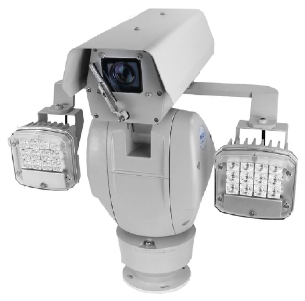
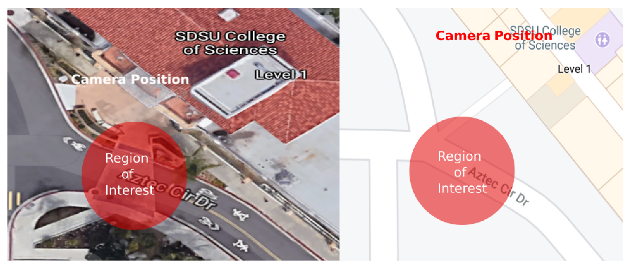
Images of pesestrians and skateboarders were obtained using a Pelco Esprit® Enhanced Series camera, shown in Figure 2. The camera was mounted on the balcony of a six-story building overlooking an intersection of two streets with sidewalks. Figure 3 shows the region of interest at San Diego State University chosen for the analysis of hazardous areas and PET calculations. A variety of road users are present, in addition to pedestrians and skateboarders, including cars, bicyclists, vans, commercial trucks, golf carts, and scooters. An object detection model is required to single out the skateboarders and pedestrians. The Pelco Esprit is capable of capturing “Full HD” 1080p ( 1920 × 1080 pixels) at 60 frames per second (fps). Captured video was compressed using H.264 “High Profile” encoding.

3. Data Distribution

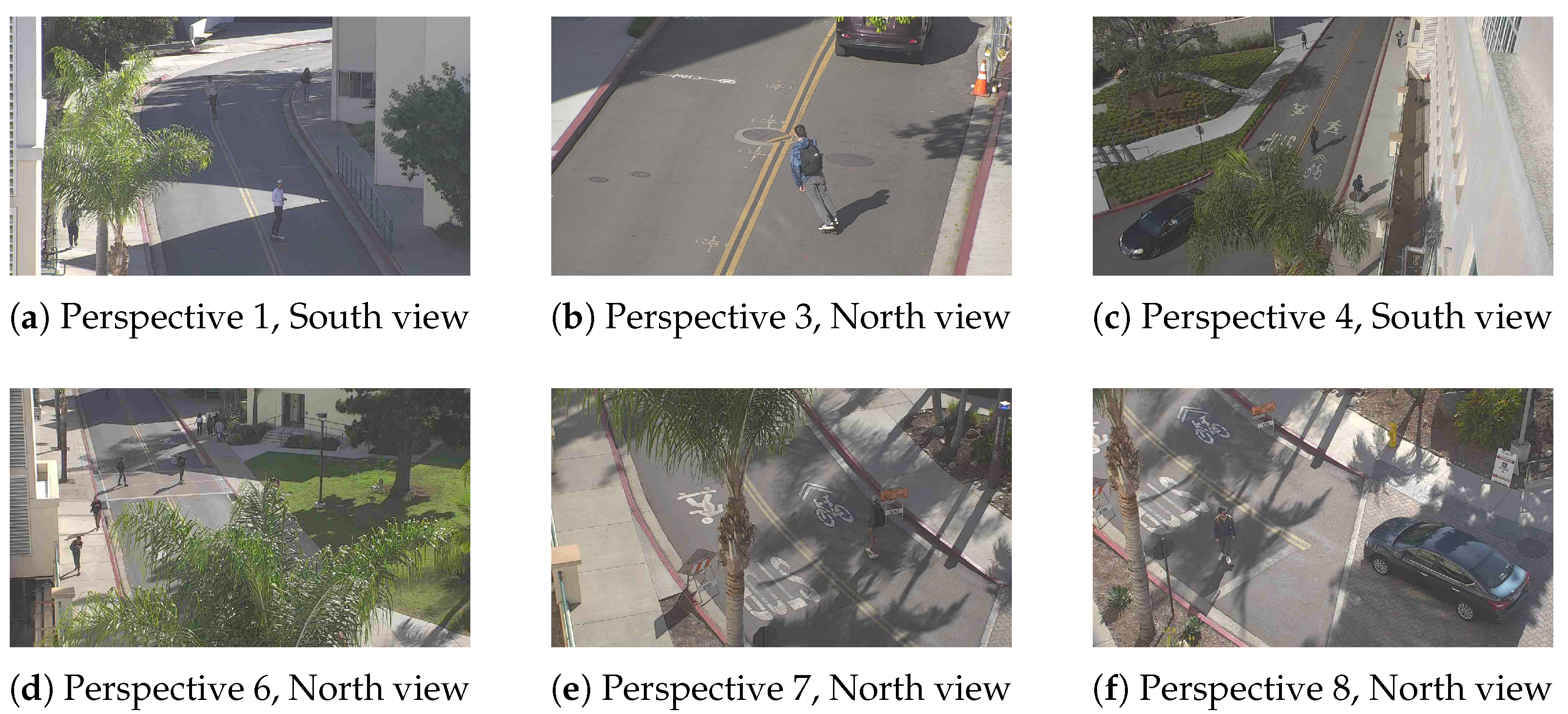
In our previous work [23], we created a new dataset with over 10 thousand images and nearly 30 thousand bounding box annotations of pedestrians and skateboarders. These images were 720p format (1280 × 720) pixels, also known as Standard HD images. In the previous work, one of the main goals was to develop the first publicly-available datasets of skateboarder images captured at multiple camera orientations. The dataset contains images taken at the eighteen pan, tilt, and zoom configurations listed in Table 1. The Pelco Esprit® is capable of 0 to 360 continuous pan rotation and + 40 to 90 continuous vertical tilt configuration. Images captured at some of these eighteen perspectives are shown in Figure 4. For this study we selected one of the perspectives used in our previous work due the good orientation for capturing pedestrian–skateboarder interactions, and used this perspective to focus on the automation of SSM calculation- and density-based hazardous region detection.
A new dataset was created that contains nearly 6500 images with over 20,000 annotations. Annotations were made using a VGG Annotator [24,25] with two class labels, pedestrian and skateboarder. The distribution of the number of annotations of skateboarders and pedestrians is shown in Figure 5. The distribution of the images captured by the time of the day is illustrated in Figure 6. Only the evening images were considered for training, since the morning and mid-day images contained shadows, making it harder for the object detection model to make predictions. A fast shadow removal algorithm is required to remove shadows, and then the images are to be fed into the object detector. Applying a shadow removal algorithm is outside the scope of this paper. Therefore, as proof of concept, only evening images were considered (images after 3:30 p.m.) when shadows were found not to impede the object detector’s performance.

4. Object Detection Models

In this section, we briefly discuss state of the art models that were fine tuned and configured to perform two different tasks: one to automate the calculation of SSMs and the other to detect hazardous regions in real-time. There has been rapid growth in deep learning research activity due to the availability of relatively inexpensive computing infrastructure, advancement in big data science, and improvement in parallel algorithms. Among the abundance of different object detection models available in the model zoo, we were tasked with identifying specific models that were convertible to use a compressed flat buffer with the TensorFlow Lite Converter, deployable to an embedded device, and able to be quantized by converting 32-bit floats to 8-bit integers. Object detection models typically solve two tasks: one is to find an arbitrary number of objects, the count of which can also be 0 (indicative of no object present in an image frame), and two, to classify and estimate the size of a detected object with a perimeter bounding box. Object detection models can be categorized into two types: two-stage models and one-stage models. Two-stage models include RCNN [27] and SPPNet [28], Fast RCNN [29] and Faster RCNN [30], Mask R-CNN [31], Pyramid Networks [32] and G-RCNN [33]. One-stage models include YOLO [34], SSD [35], RetineNet [36], YOLOv3 [37], YOLOv4 [38], and YOLOR [39]. The key difference between these two types of models is that the latter combines the two tasks into one step (hence the name one-stage object detectors) to achieve higher performance, but at the cost of accuracy. In two-stage detectors, the approximate placement of the object regions are proposed using deep features before these features are used for classification and determining the bounding box. Two-stage detectors achieve higher accuracy, but are generally computationally slower. One-stage detectors predict the location and dimension of bounding boxes without the region proposal step and therefore require less computational time and are suitable for real-time applications. These detectors prioritize inference speed and are extremely fast, but are not as capable in recognizing irregularly shaped objects. In our practical application of pedestrian and skateboarder identification, we need to leverage deep learning models to perform two tasks: one to automate the calculation of SSMs, which require the detection of skateboarders and pedestrians with high accuracy, and two, to detect hazardous regions in real-time which requires choosing of a model that will execute in real-time. The Faster R-CNN model is known for its high accuracy and therefore we chose this model for the first task. For the second task we chose the SSD model, as it is known for having low inference and fast processing time. In addition, since we want to make our model edge-based (for example, deployable on the Google Coral USB Accelerator and Google Edge TPU Dev Board [40]) so that we can connect a device deployed with the model directly to a camera, we also chose a model that is TPU compatible. These edge devices support the Tensorflow Object Detection API. For this reason, we identified two variants of the SSD model supported by the Tensorflow Object Detection API that are suitable for the practical application of real-time, edge-based pedestrian and skateboarder identification for the calculation of SSMs at traffic intersections.
As mentioned above, the Faster Region-based Convolutional Neural Network (Faster R-CNN) and two variants of the Single Shot Multi-box Detector (SSD) deep learning models were used for the detection and classification of both pedestrians and skateboarders and the Tensor Flow Object Detection (TFOD) API [41] was used to train our dataset. A detailed explanation of the two architectures of the Faster R-CNN and SSD can be found in [30,35], respectively. After careful consideration, we trained three models for the purpose of automated calculation of PET and hazardous region detection; the Faster R-CNN ResNet model, the SSD MobileNet V2 model, and the SSD MobileNet V1 model. For brevity, in the remainder of this article, the models will be called Faster R-CNN, SSDV2, and SSDV1lite (“lite” to indicate the model is TPU compatible).

5. Performance Metric of Object Detection Models

Evaluation of object detector model performance is based on the combination of two evaluation metrics: Intersection over Union (IoU) [42] and mean Average Precision (mAP) [43].
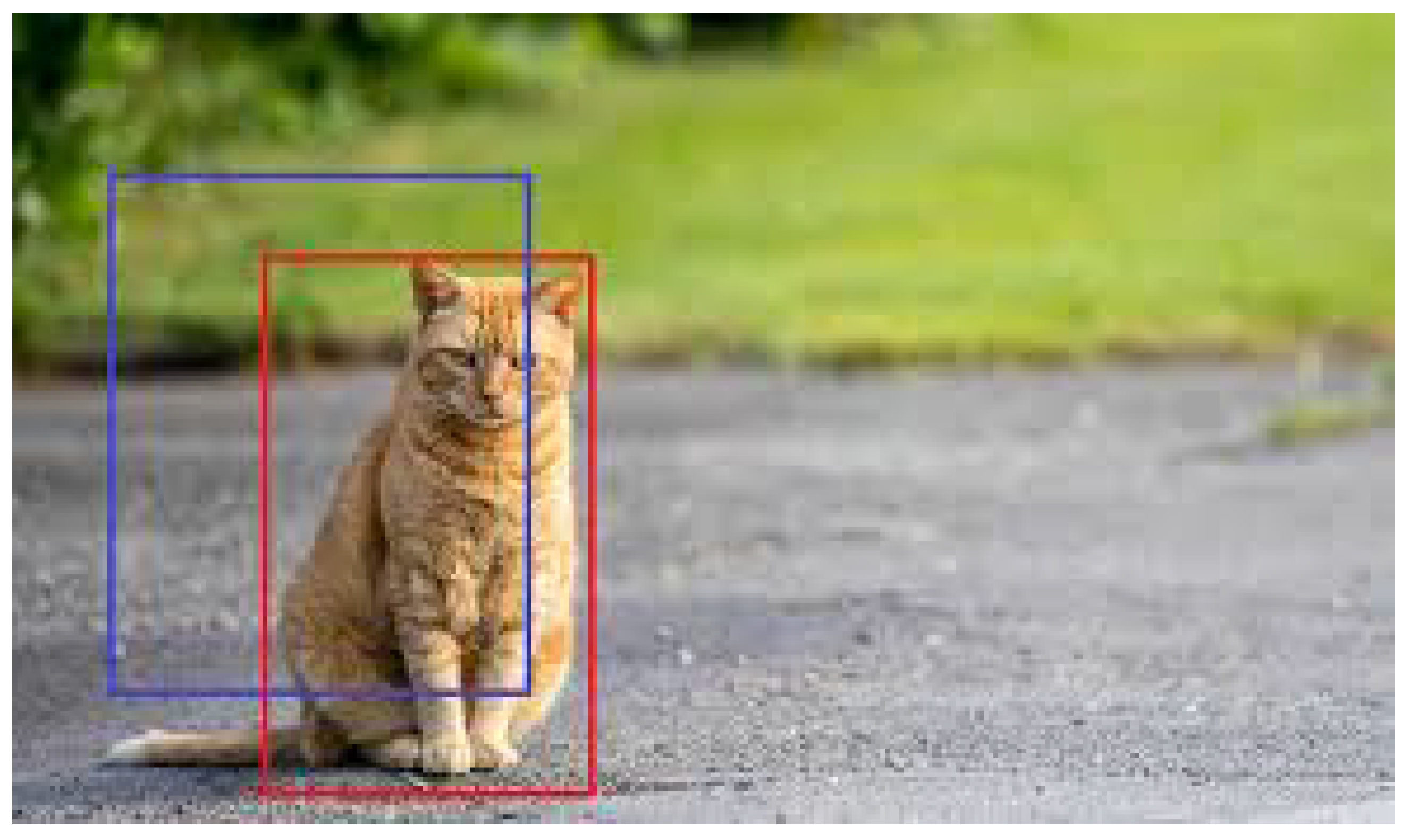
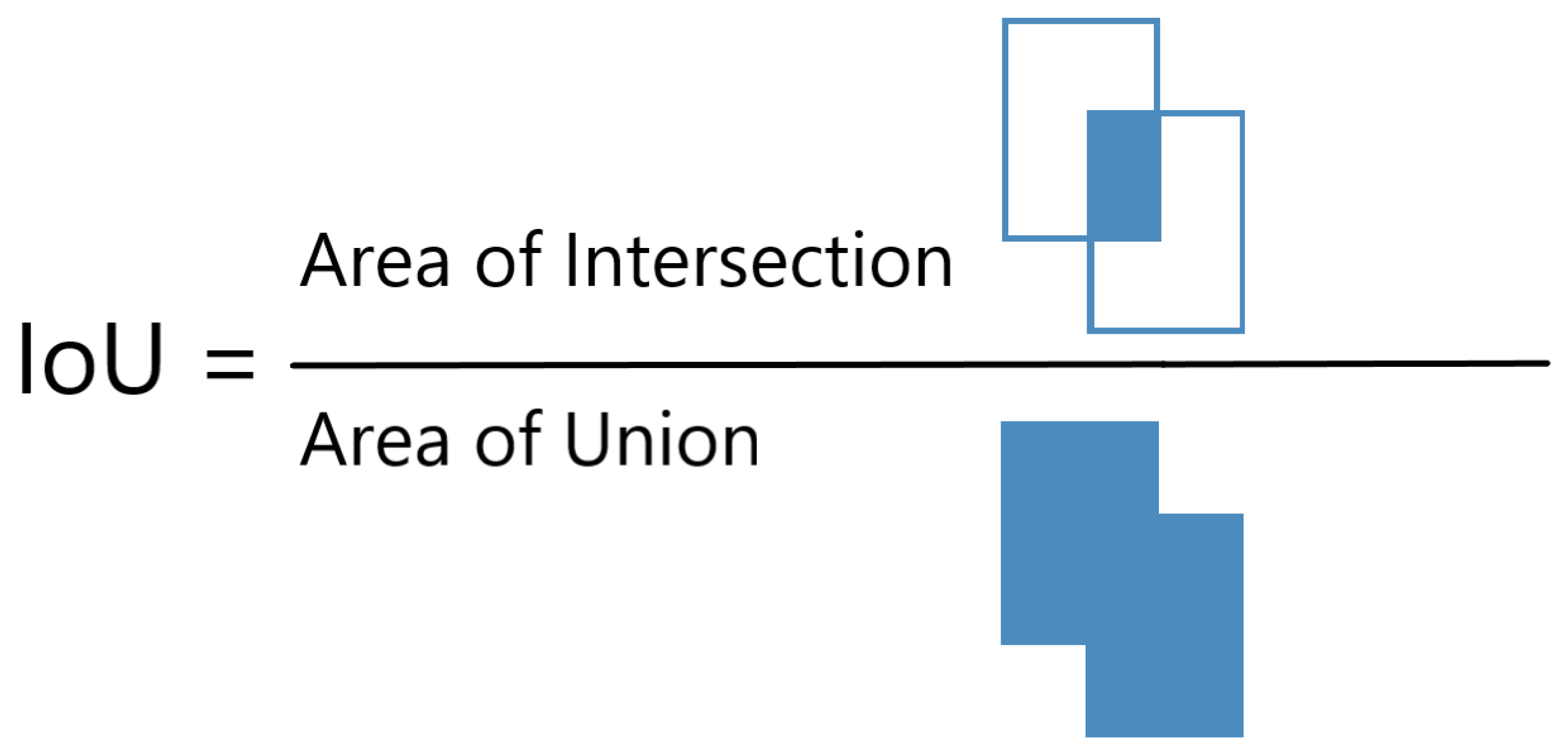
In Figure 7, the red bounding box denotes the ground truth bounding box, and the blue box indicates the predicted bounding box by an object detector. The IoU, as Figure 8 illustrates, is simply the ratio of the area of intersection in the union of these two bounding boxes. The greater the value of overlap (numerator), the higher the IoU. An IoU of greater than 0.5 is considered to be an above-average prediction. The mAP is another evaluation metric used for object detection. The calculation of the mAP is based on values of precision and recall. Precision is the number of correctly predicted objects in an image. Recall determines the ability of the detector to find all the images in the image. The precision and recall values depend on the metrics True Positive (TP), True Negative (TN), False Positive (FP), and False Negative (FN). A TP finding indicates the detector correctly predicted an object. TN means the detector is correctly detecting the absence of an object. FP means the detector is falsely predicting the presence of an object when there is none. Finally, FN means the detector is failing to report the locations of one or more actually present objects. Equations (1) and (2) are used to calculate precision and recall.
P r e c i s i o n = T P T P + F P
R e c a l l = T P T P + F N

6. Results

This section discusses the input size of the different models, the performance of the models in terms of mean average precision (mAP), the hardware and model frame rates, the training loss and evaluation loss of the models, and model prediction on new images. Critical findings are analyzed and highlighted. Based on the results, in the next section, two suitable models out of three are selected for two separate tasks: automated calculation of Post Encroachment Time (PET) and finding hazardous conflict zones in real-time.

6.1. Model Input Size

The Faster R-CNN model takes as input an image of dimensions 1920 × 1080 . For the SSDV2 model, the image is resized to 300 × 300 , as the model only accepts as input an image of dimension 300 × 300 . In the SSDV1lite model, the image is resized to dimensions 640 × 640 , as this model only accepts as input an image of dimensions 640 × 640 . For both SSD models, there is a loss of information when size is reduced, which may affect object classification accuracy.

6.2. Model Mean Average Precision

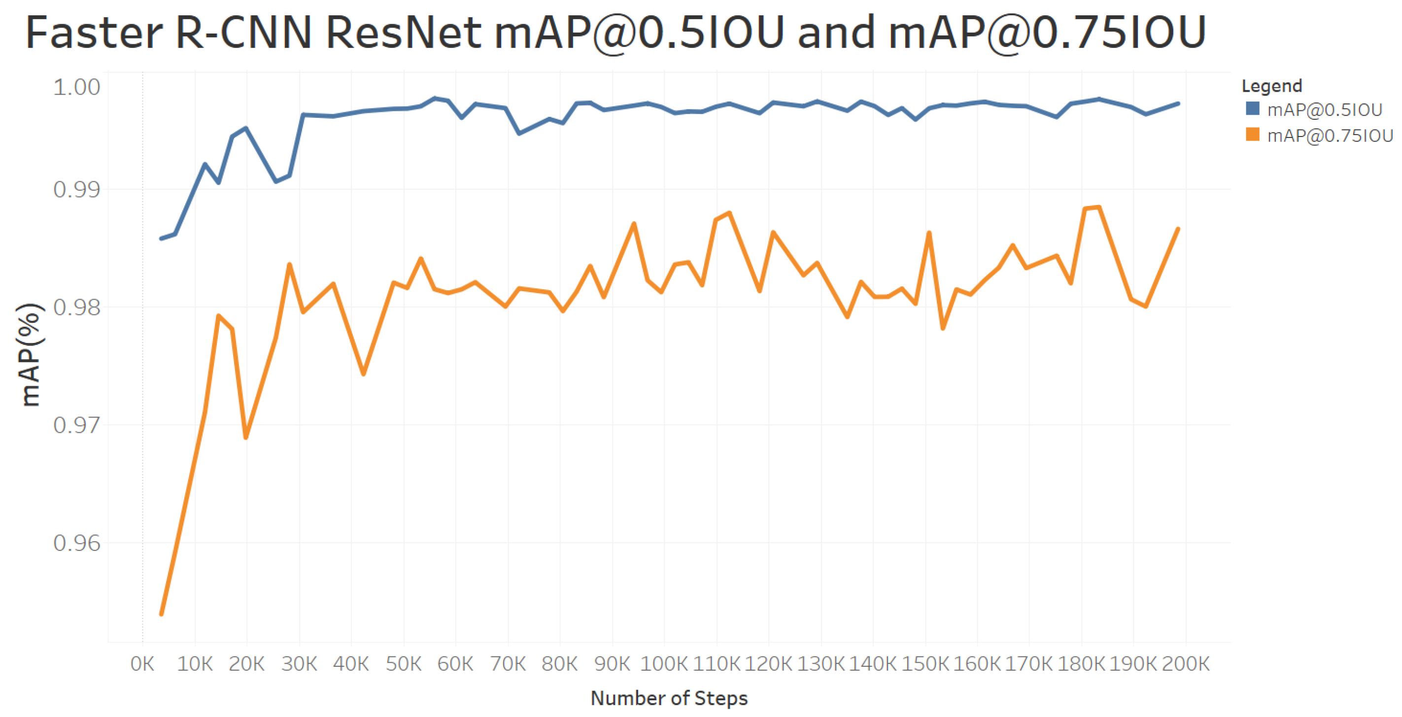
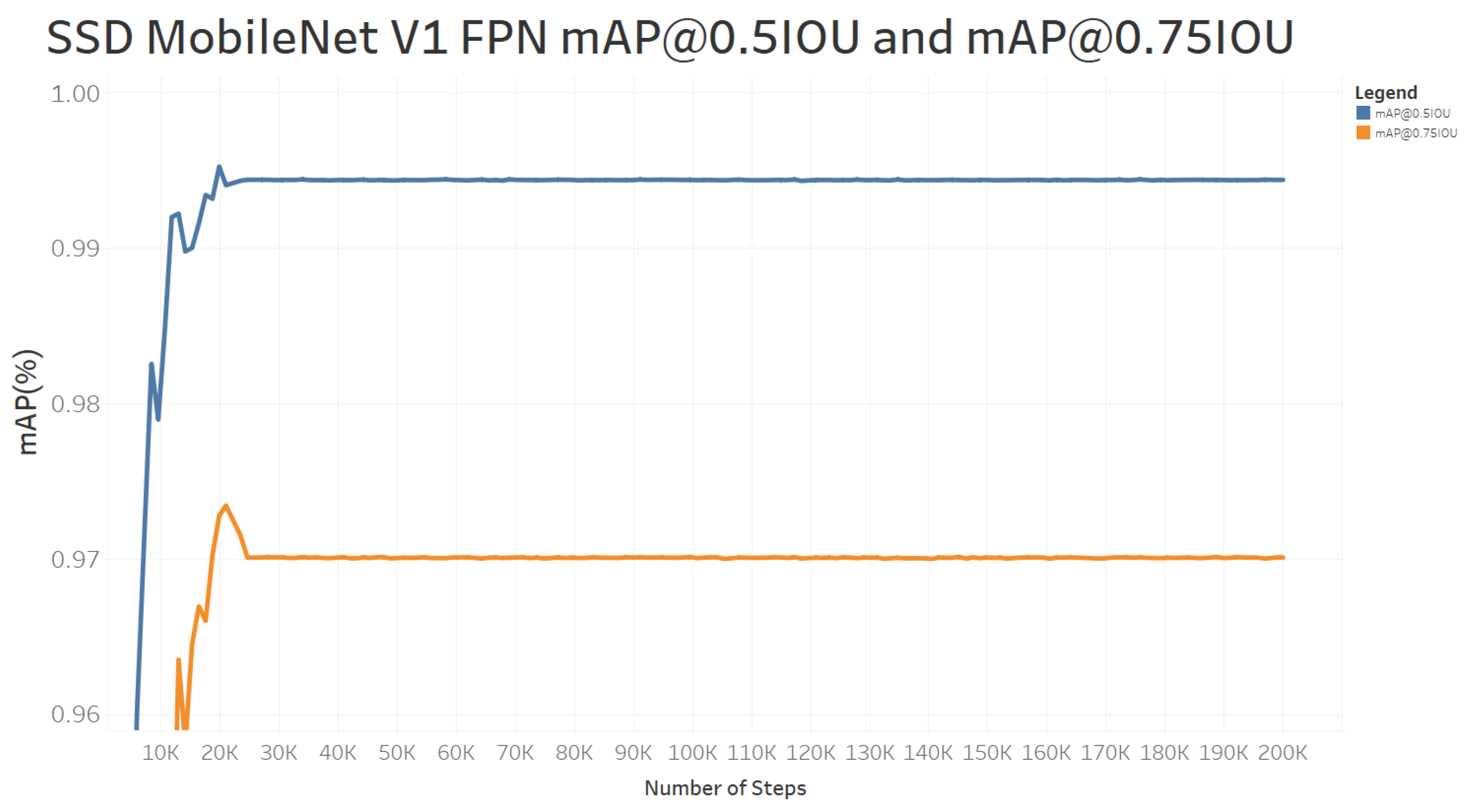
Evaluation of object detector model performance is based on the combination of two evaluation metrics: Intersection over Union (IOU) [42] and mean Average Precision (mAP) [43]. All three models were run for 200,000 steps. From Figure 9 it can be observed that the Faster R-CNN model stabilizes at an mAP above 99.5% at 0.5 IoU and oscillates above 98% at 0.75 IoU by the end of the training period. The SSDV2 model reaches a mAP of 98% at 0.5 IoU and oscillated around 92% at 0.75 IoU, as shown in Figure 10. The SSDV1lite settles just a little under 99.5% at 0.5 IoU and 97% at 0.75 IoU, as shown in Figure 11. With respect to the mAP performance metric, the Faster R-CNN model excels over the other two models, and the SSDV1lite model performs better than the SSDV2 model.

6.3. Hardware and Model Frame Rates

A total of 194 images were accumulated from the test set and all three models were used to predict pedestrians and skateboarders while recording elapsed time and frame rate (fps). The results are tabulated in Table 2 and were obtained using NVIDIA® V100 Tensor Core GPUs, powered by the NVIDIA® Volta architecture. From Table 2, the Faster R-CNN model has the slowest processing frame rate and is not suitable for real-time deployment. The SSDV1lite model, on the other hand, has a relatively fast frame rate and is able to process 102 frames per second, which makes this model suitable for real-time classification.

6.4. Model Training Loss and Evaluation Loss

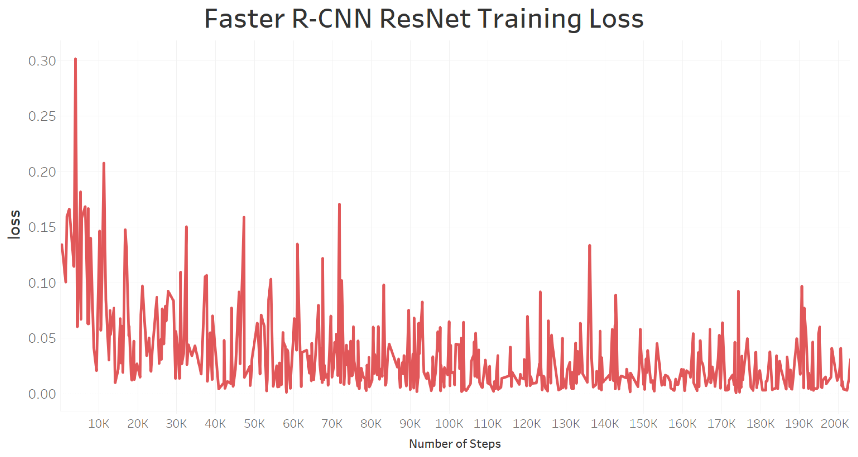
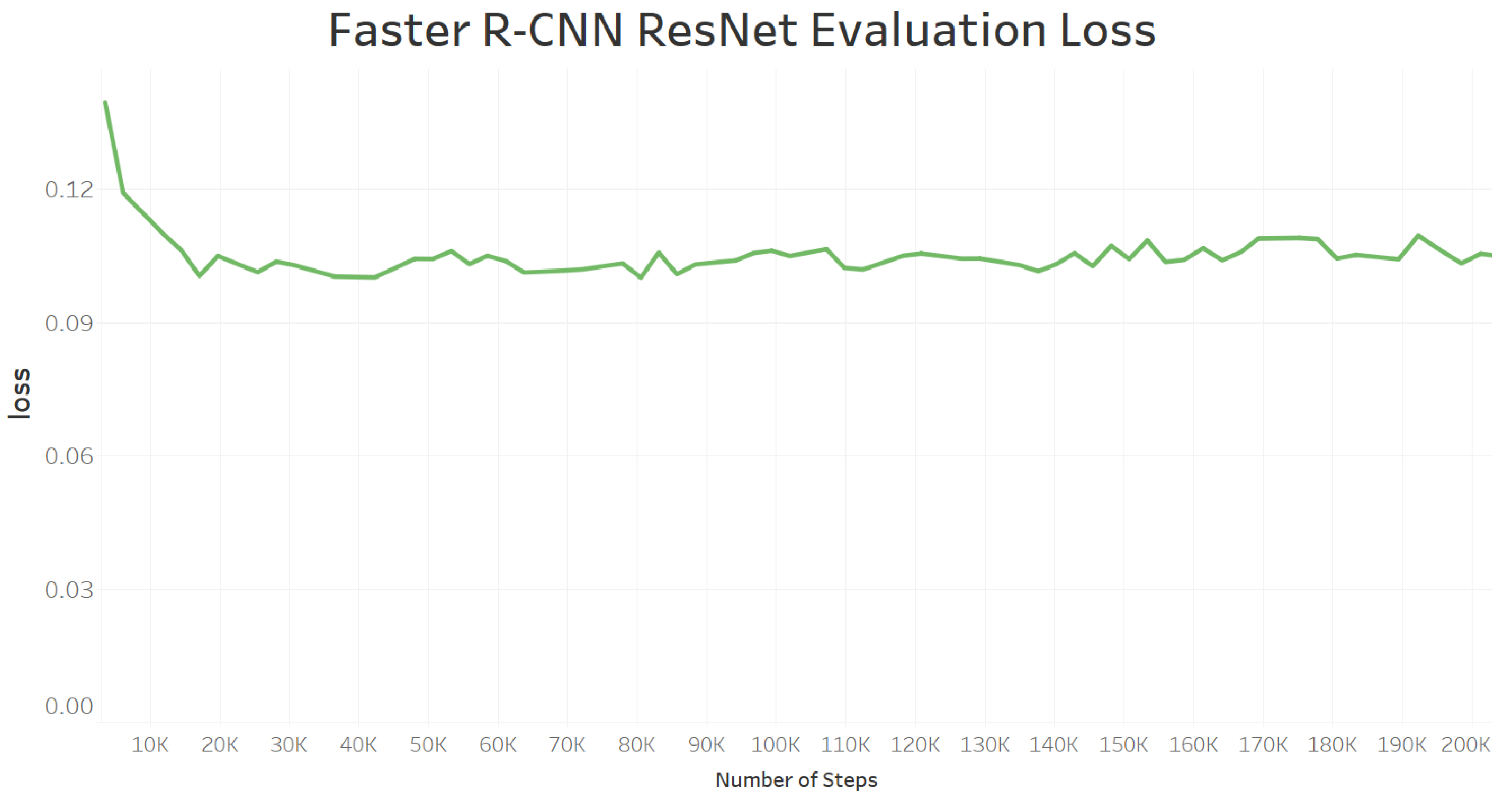
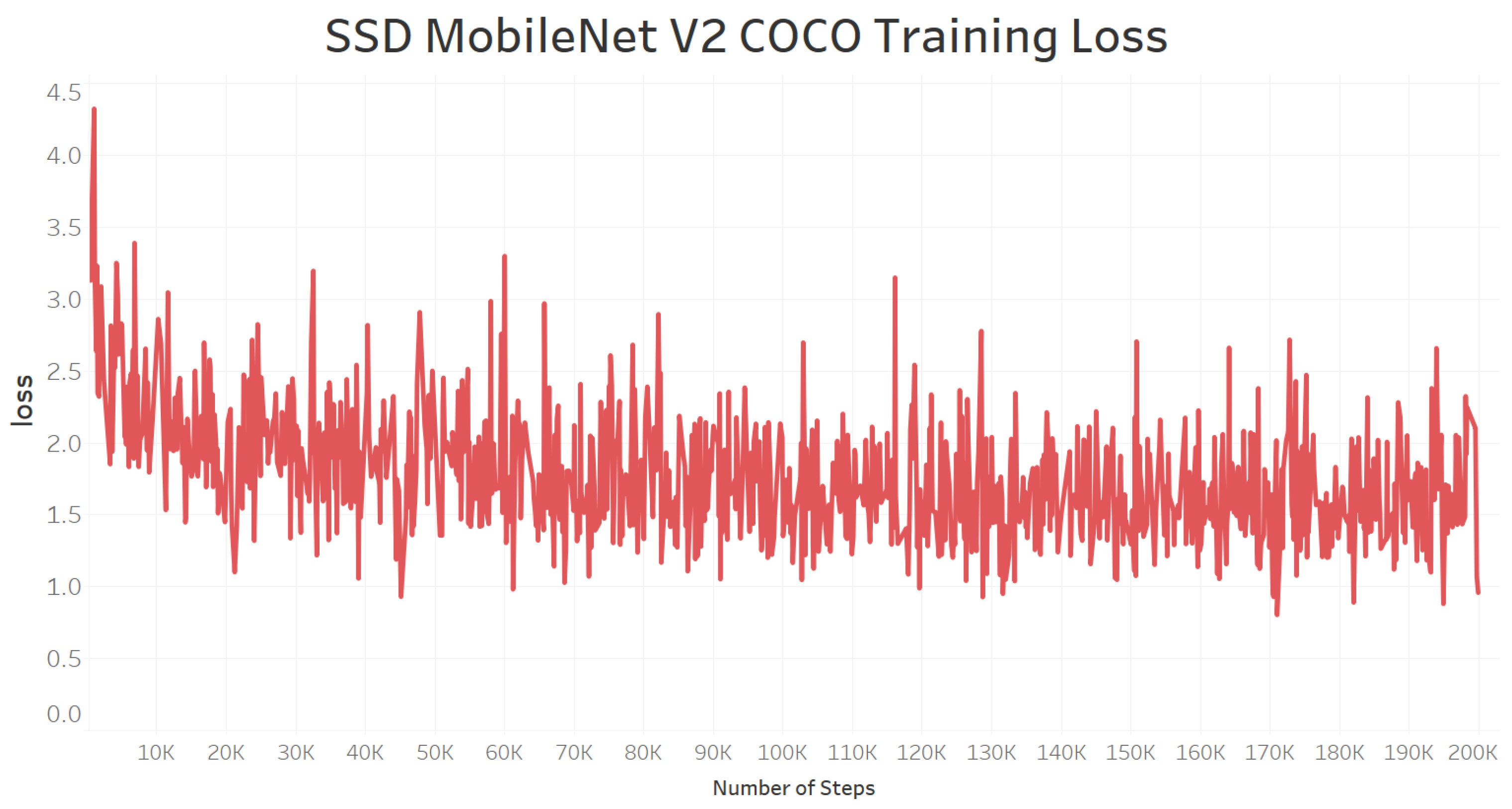
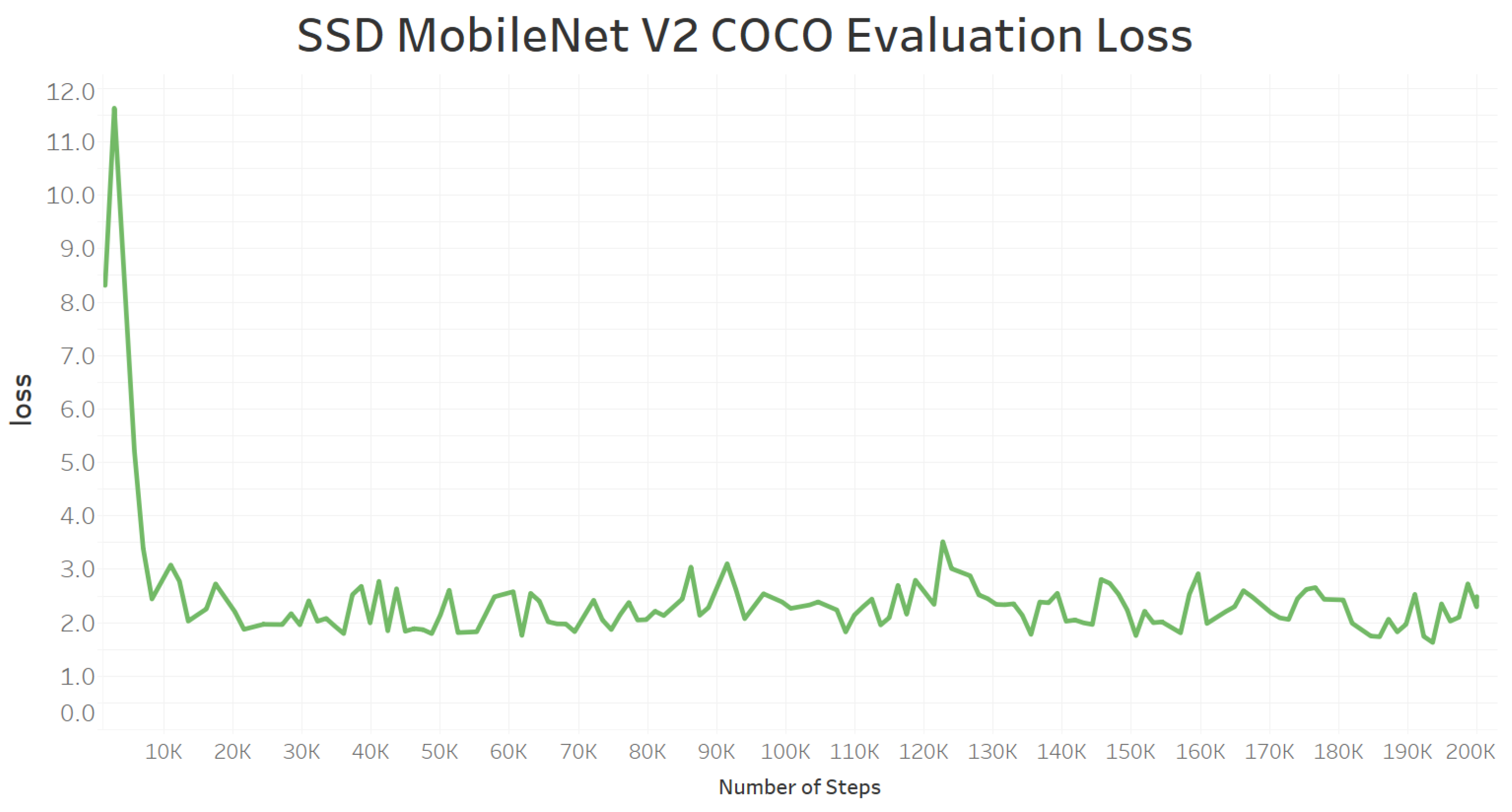
Training loss for the Faster R-CNN model starts low and then decreases to nearly 0.00, as shown in Figure 12. The evaluation loss shown in Figure 13 illustrates the loss is around 0.1. Because the training loss and the evaluation loss are close in value, we can assume no over-fitting is occurring. Figure 14 demonstrates the training loss of the SSDV2 model, and the loss by the end of 200,000 steps is slightly above 1.00. The evaluation loss shown in Figure 15 for the same model by the end of the training is around 1.80. Again, both values being in the neighborhood of each other indicates no over-fitting is occurring. Finally, for the SSDV1lite model, the training loss shown in Figure 16 is around 0.13 and, as shown in Figure 17, the evaluation loss is around 0.2. It can be observed that the model does not have an over-fitting problem. The Faster R-CNN and SSDV1lite models are shown to be more reliable than the SSDV2 model.

6.5. Model Prediction Evaluation

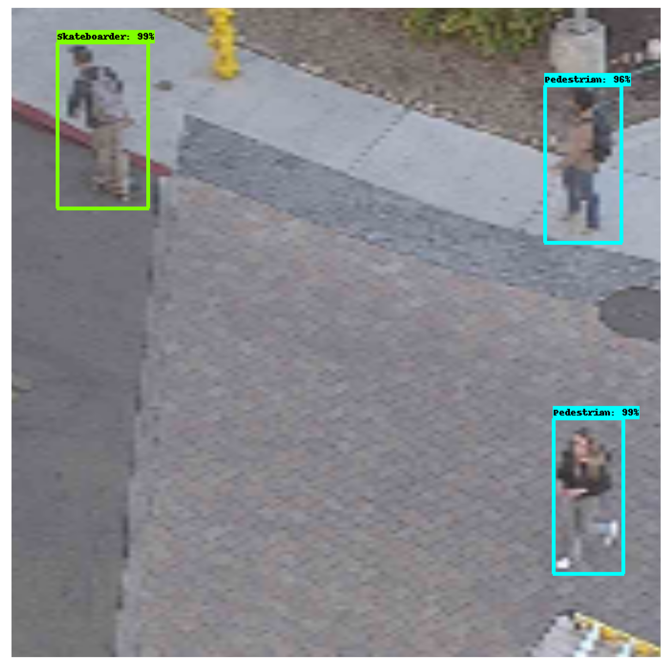
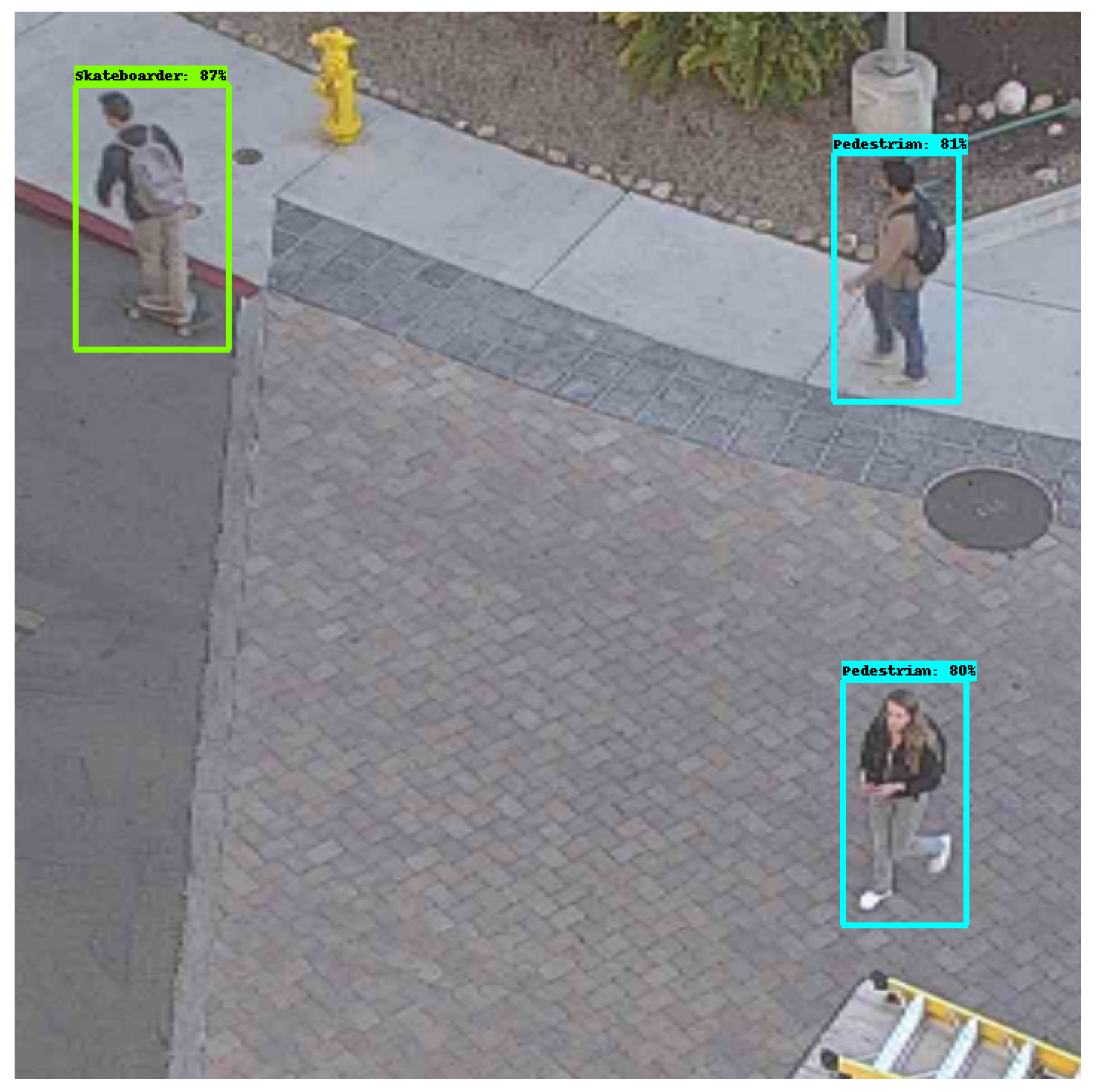
The same image has been used for the three models to show their difference in performance. The Faster R-CNN model, as shown in Figure 18, predicts the three objects correctly in the image (one skateboarder and two pedestrians) with a confidence of 99% for all objects. Figure 19 shows that the SSDV2 model evaluates the skateboarder with a confidence of 99%, one pedestrian at 96%, and the other pedestrian at 99%. The reduction of the images to dimension 300 × 300 from the original dimension is the reason for the image pixelation. The SSDV1lite model predicts skateboarders with a confidence of 87% and the two pedestrians with a confidence of 81% and 80%, as seen in Figure 20. Based on model performance, it can be observed that the Faster R-CNN model, in terms of accuracy, excels over both models. While the SSDV2 model performs well in this particular example, the model exhibits a high loss compared to the other models, which means the model has a higher chance of misclassifying a skateboarder as a pedestrian, and vice-versa. The SSDV1lite has an extremely low loss measure compared to the SSDV2 model, which makes the model more reliable.

6.6. Critical Findings Summarized

The main findings are summarized in this section. Table 3 summarizes the mean average precision of the three models, the evaluation loss, and the observed processing frame rate. It can be observed that the Faster R-CNN model has the highest accuracy in terms of [email protected] IoU and [email protected] with a very low loss, but has an extremely slow frame rate of only 35 fps. The SSDV2 model has [email protected] and [email protected] at 98% and 92%, respectively, but has a higher loss of 1.8. This implies the model is likely to make more errors when classifying new images. This model has a frame rate of 54 fps. Finally, SSDV1lite exhibits a high accuracy with [email protected] and [email protected] at 99.5% and 97%, respectively, with a low loss. This model also has a relatively high frame rate of 102 fps. Moreover, because this particular model is TPU-compatible, it can perform inferencing in situ. In the next section we discuss how we select two models out of the three trained models to perform two very different tasks: automated PET calculation, and real-time hazardous conflict zone determination. The first task requires high precision, while the later task requires real-time capability.

7. Model Selection and Application

In this section, we choose two suitable models out of the three for two very different tasks: one model to automate the calculation of PET and the other model to detect hazardous conflict zones in real-time.

7.1. Automated PET Calculation

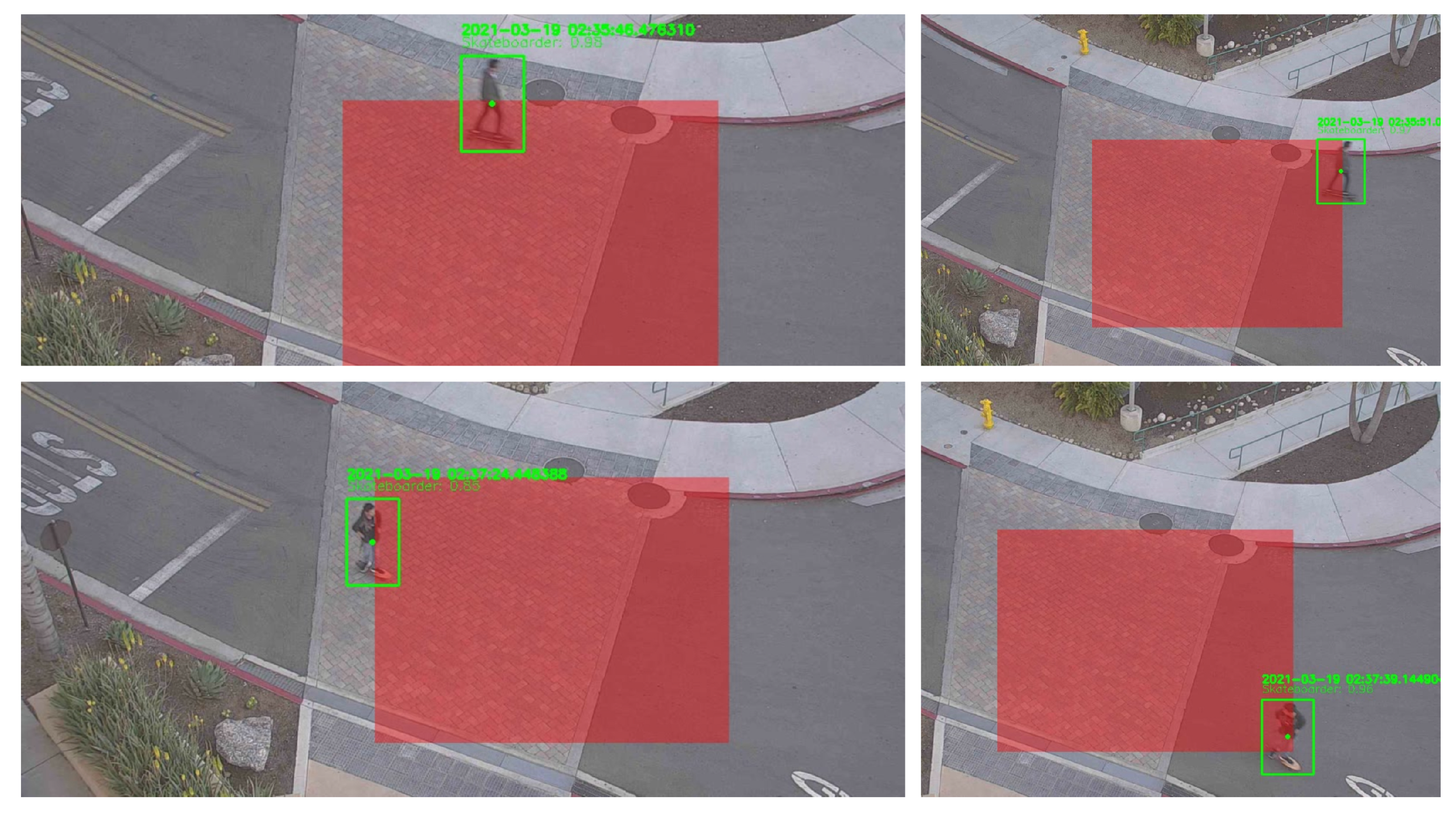
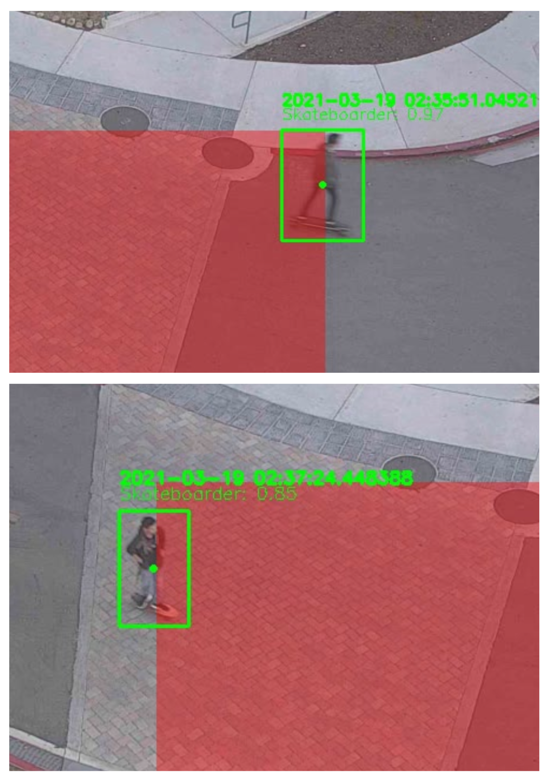
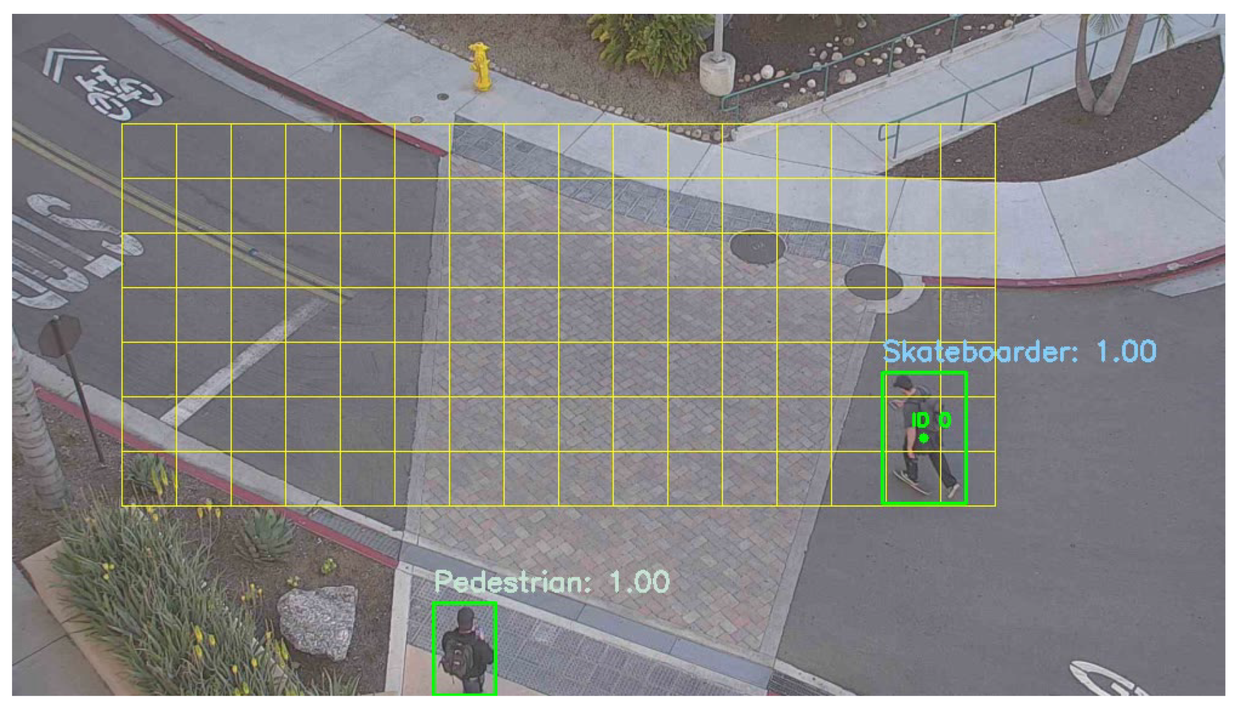
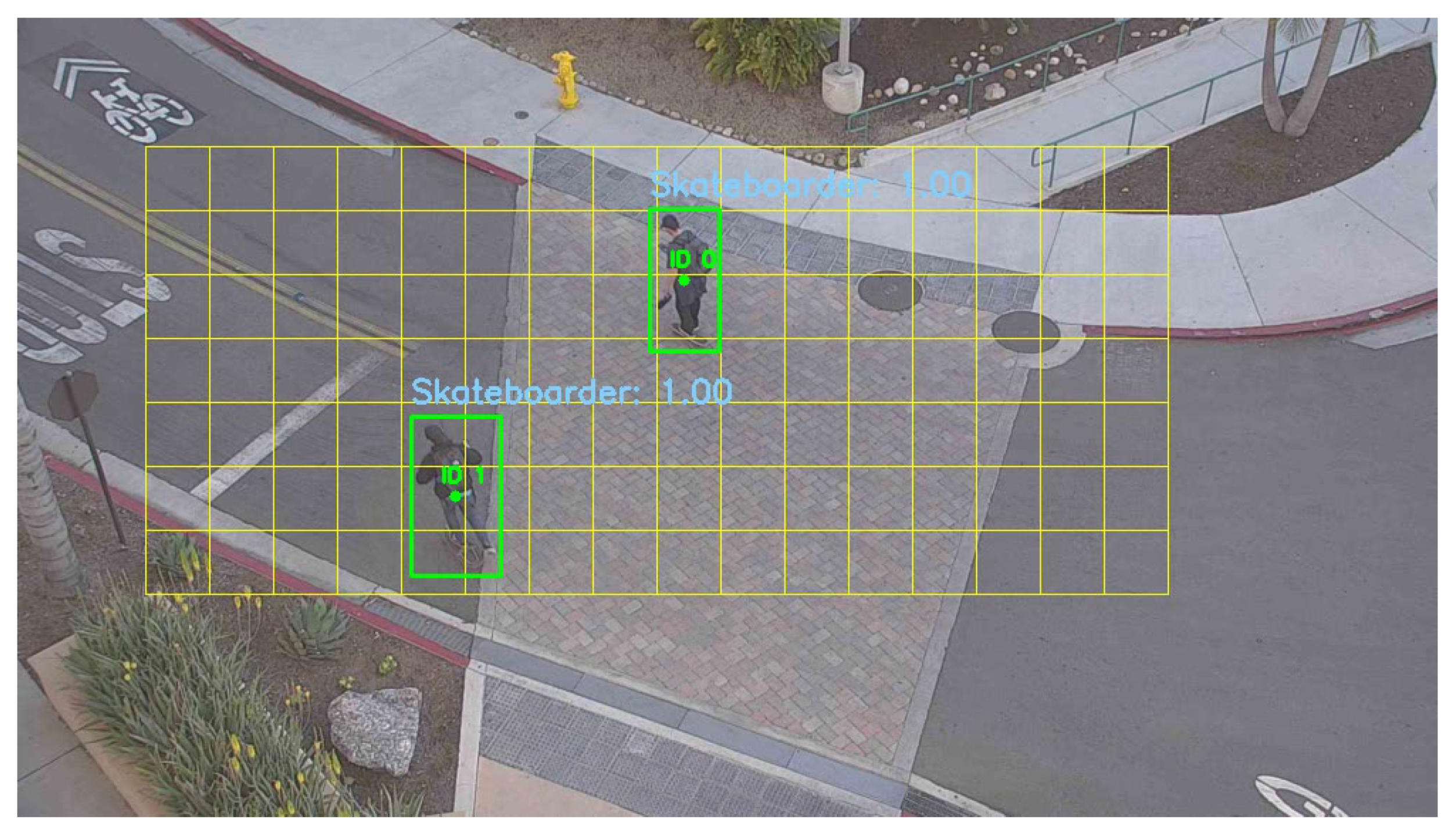
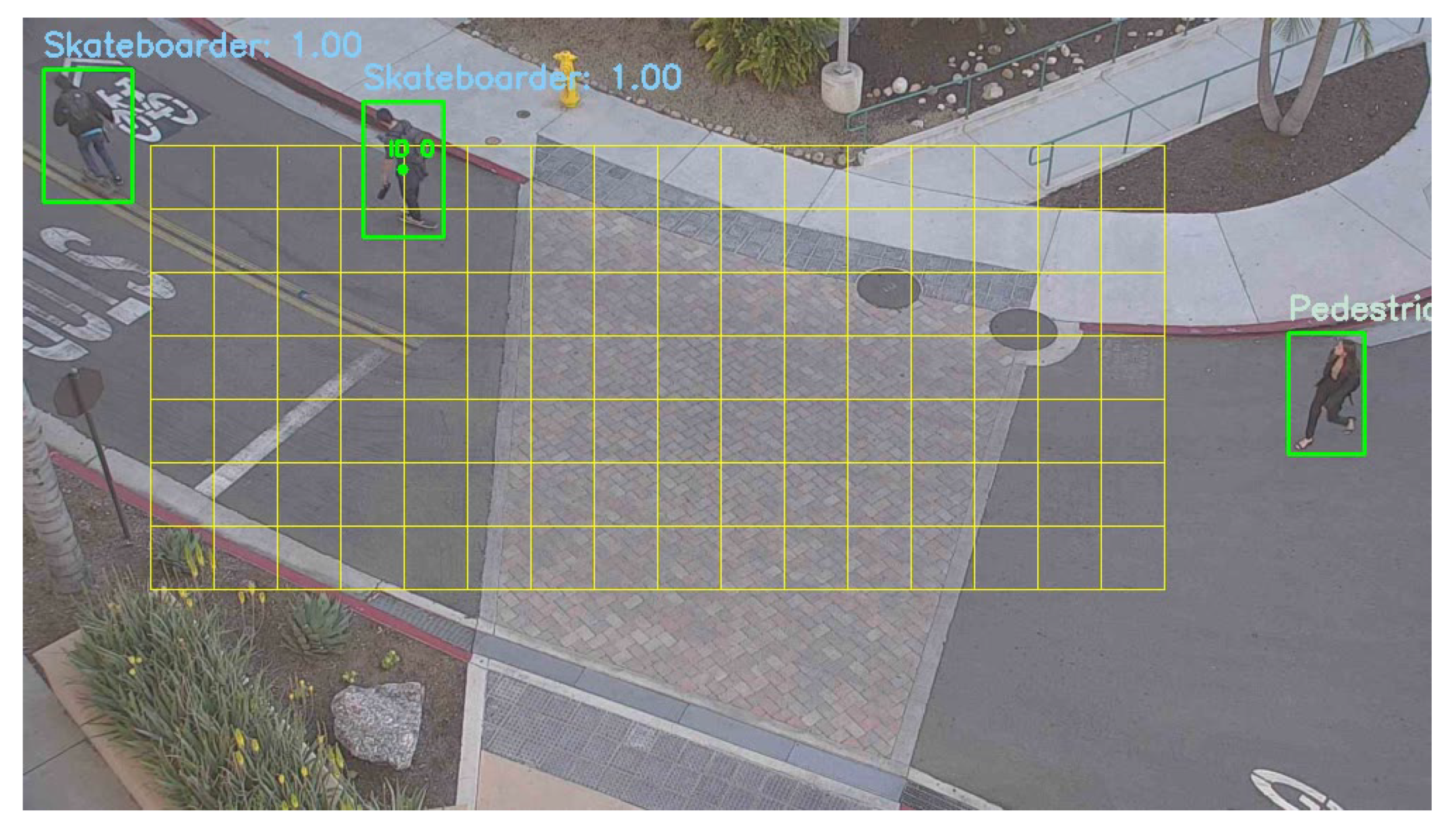
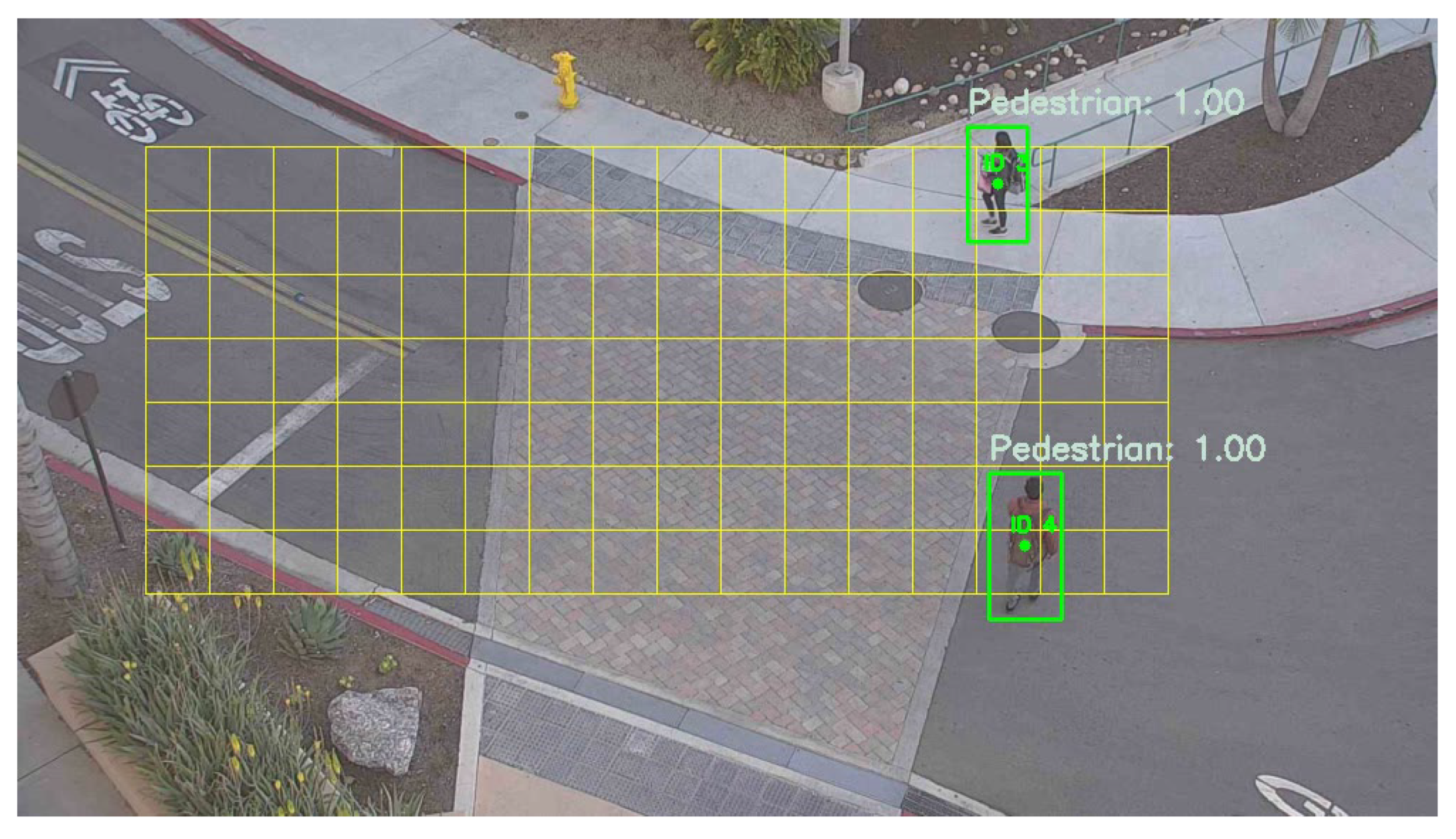
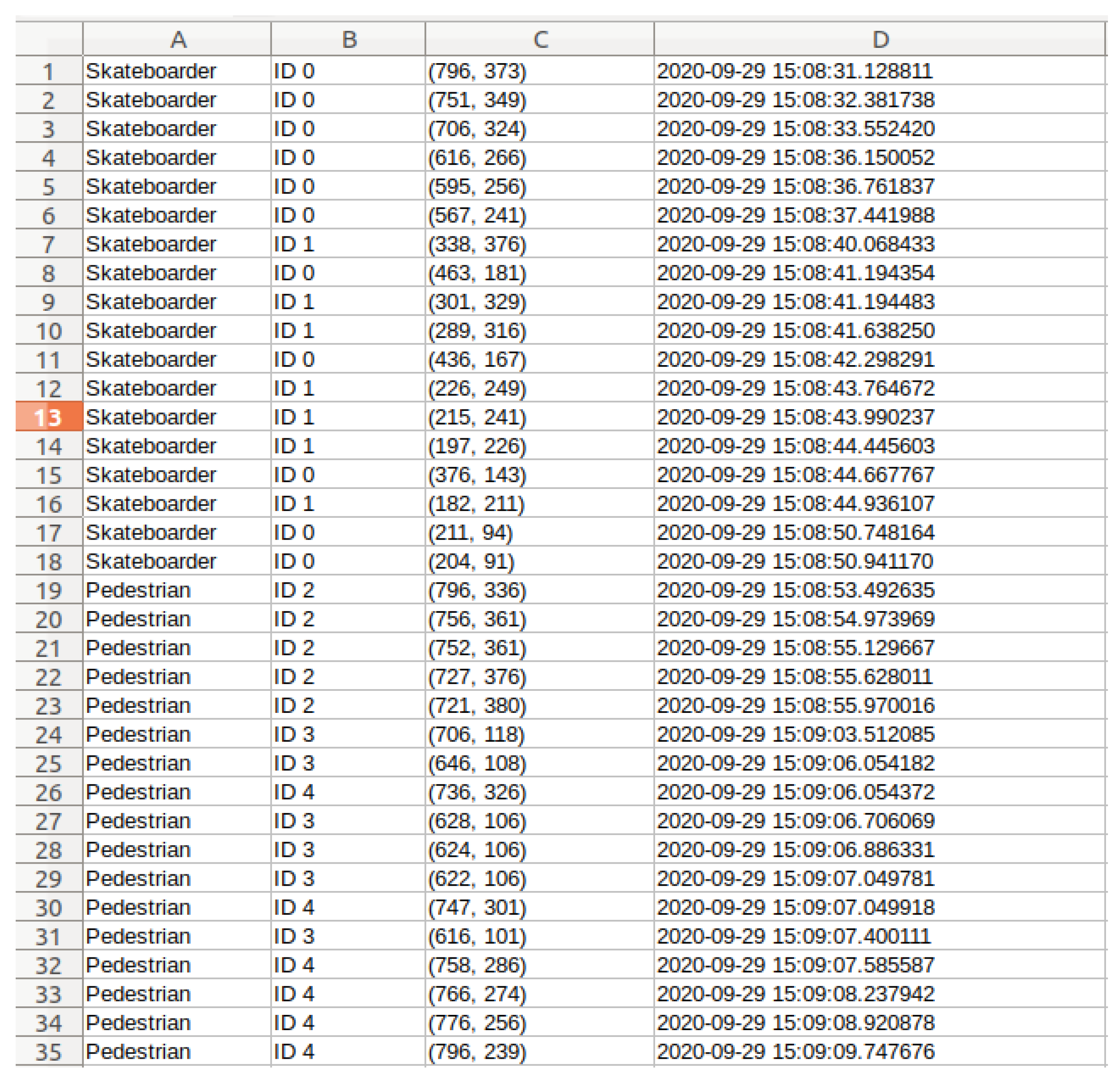
For each location recorded for the leading vehicle, the PET is calculated as the time difference between the arrival of the leading vehicle at that location and the arrival of the following vehicle at that location [46]. Figure 21 is analogous to Figure 1. In Figure 21 we have a pair of skateboarders entering and leaving a superimposed artificially created conflict zone shown in red. The top portion of Figure 22 shows the first skateboarder leaving the conflict zone and the bottom portion shows a following second skateboarder entering the conflict zone. The ingress and egress time of both these objects are recorded. The egress time for the first skateboarder occurs at 2:35:51.04, while the ingress time of the following skateboarder occurs at 2:37:24.44. Therefore, PET for this pair of objects is Δ t = 2:37:24.44 − 2:35:51.04 = 93.4 s. PET calculation for skateboarder and pedestrian objects requires recording of the time each pair of objects enters and exits (ingress and egress) an area, the ID of each object, the (x,y) coordinates of each object, and the class (label) of each object. A grid is drawn over the road area where pedestrians and skateboarders pass. Instead of rendering a grid over the entire screen, the grid is rendered only over a potential conflict area. The reason can be explained by looking at Figure 23. Notice how the object at the bottom is detected as a pedestrian. However, the same object is detected as a skateboarder after additional frames elapse, as shown in Figure 24. This is due to the occlusion problem. The object detector partially can see the object and detects it as a pedestrian. Only after the detector sees the pedestrian with a skateboard does it classify the object as a skateboarder. Let us assume that the ID registered on the pedestrian is one. When the pedestrian is in full view, the object will be detected as a skateboarder, and it would be registered with ID two. This would be wrong because the model is classifying the same object initially as a pedestrian and then as a skateboarder, therefore affecting the calculation of PET. PET calculation requires precision. This is why the object detector is provided with some free-space to allow the complete object to appear before an ID is registered to an object. This can be seen in Figure 23, where the object entering the grid space has been registered while the pedestrian outside the grid has not been registered. The pedestrian is only correctly registered with ID 1 and with proper classification, as illustrated in Figure 24, when the pedestrian enters the grid region. In Figure 25, when ID 1 leaves the grid, the pedestrian is de-registered. In addition, in the same figure, we can see a pedestrian entering the scenario, and because the pedestrian is outside the grid region, the pedestrian has not been registered yet. Figure 26 demonstrates two pedestrians registered as soon as they are in the grid region. The PET calculation requires the class, ID, (x,y) coordinates, and the time the object enters and leaves the grid. Figure 27 shows how objects are being recorded as the simulation is running. Finally, all data are automatically collected and stored in a Microsoft Excel file, as shown in Figure 28, and this can be provided to a civil engineer to calculate PET offline. It is of paramount importance that the object detector accurately classifies each object because any misclassification would affect the PET calculation. The Faster R-CNN model also provides stable detection and classification in every frame. Therefore, out of the three models, the Faster R-CNN model is the best model to be considered for this purpose. Despite its high accuracy, the fps of the Faster R-CNN model is relatively slow. Therefore, an Excel sheet can be generated after running the model on recorded video that captures real-time scenarios.

7.2. Real-Time Hazardous Conflict Zone Determination

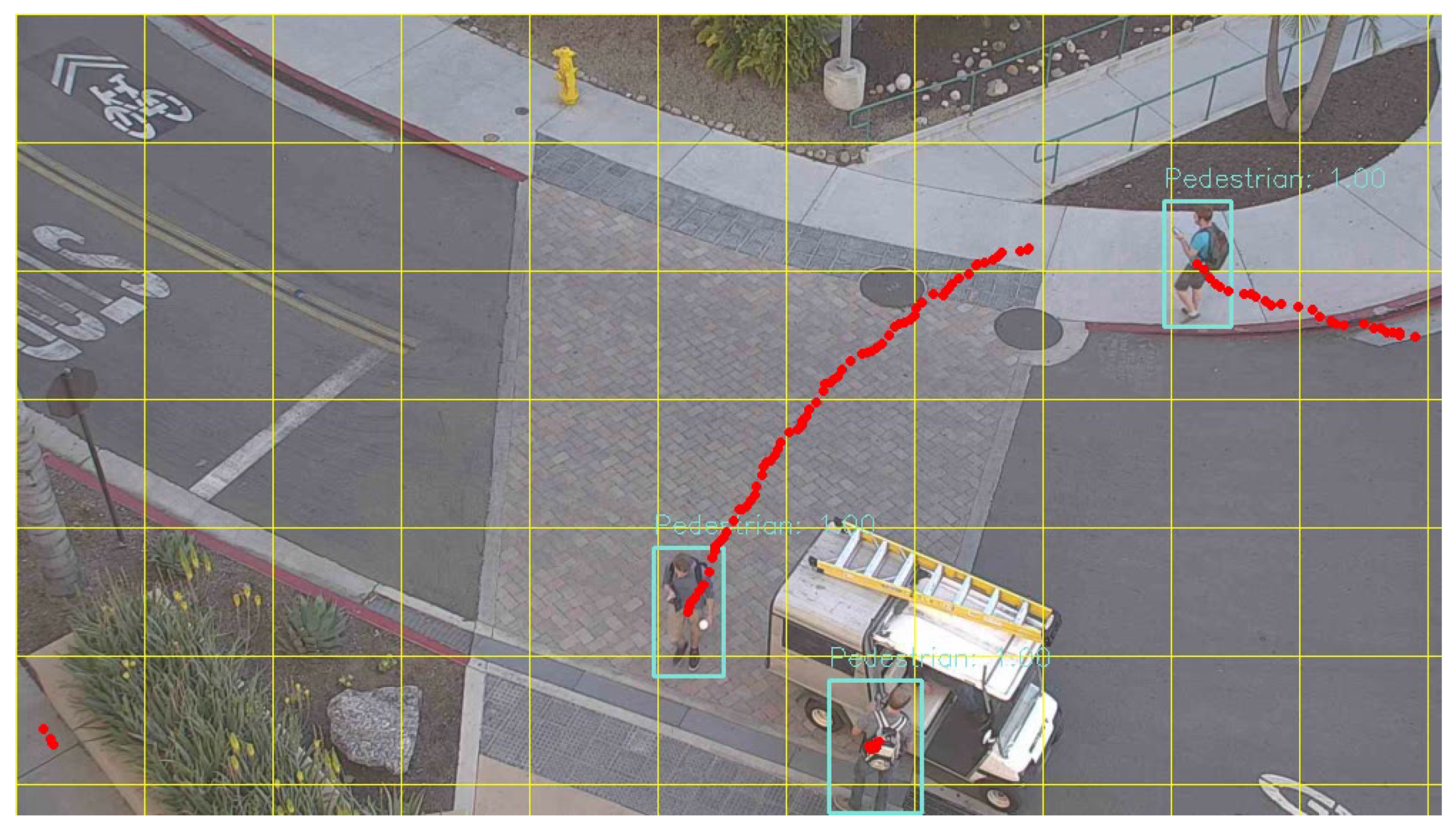
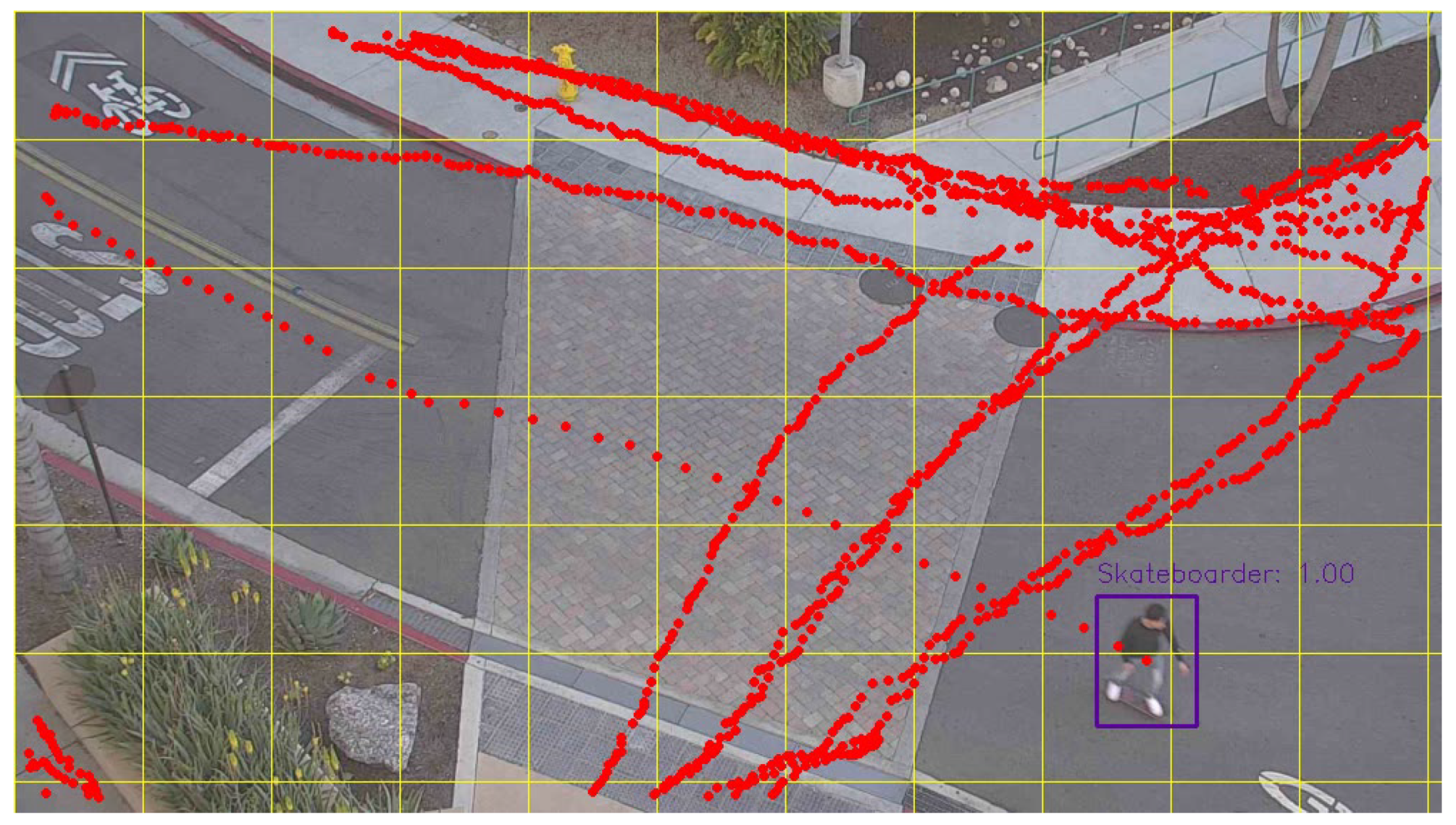
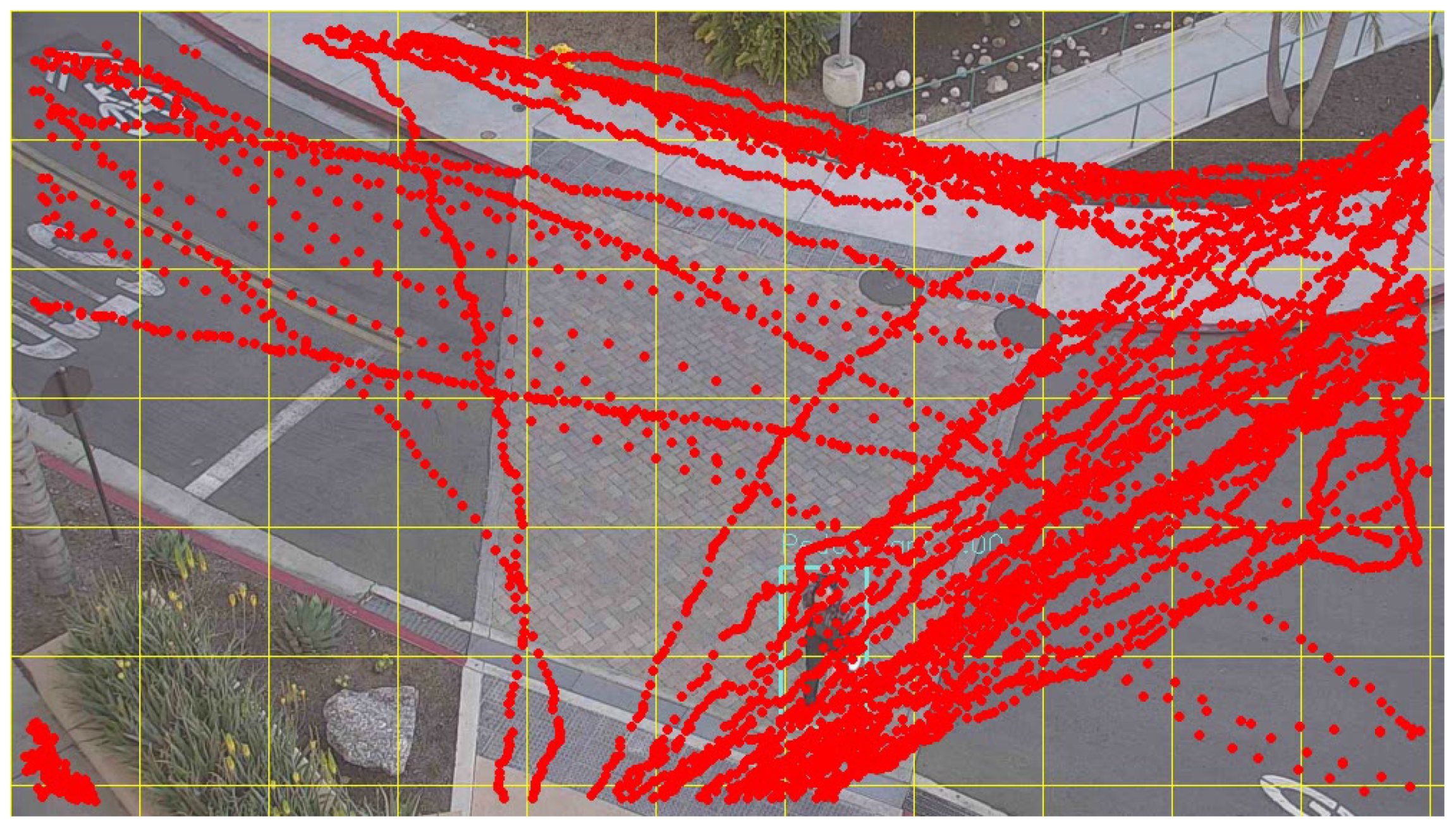
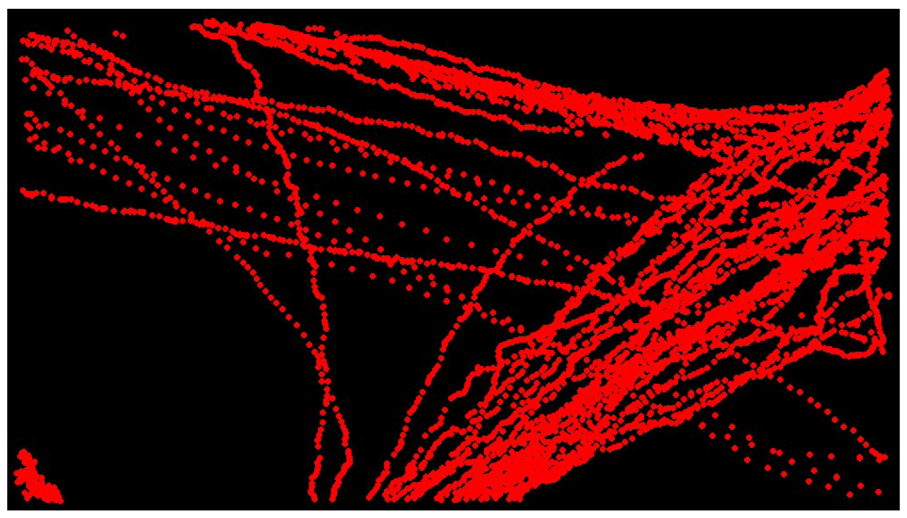
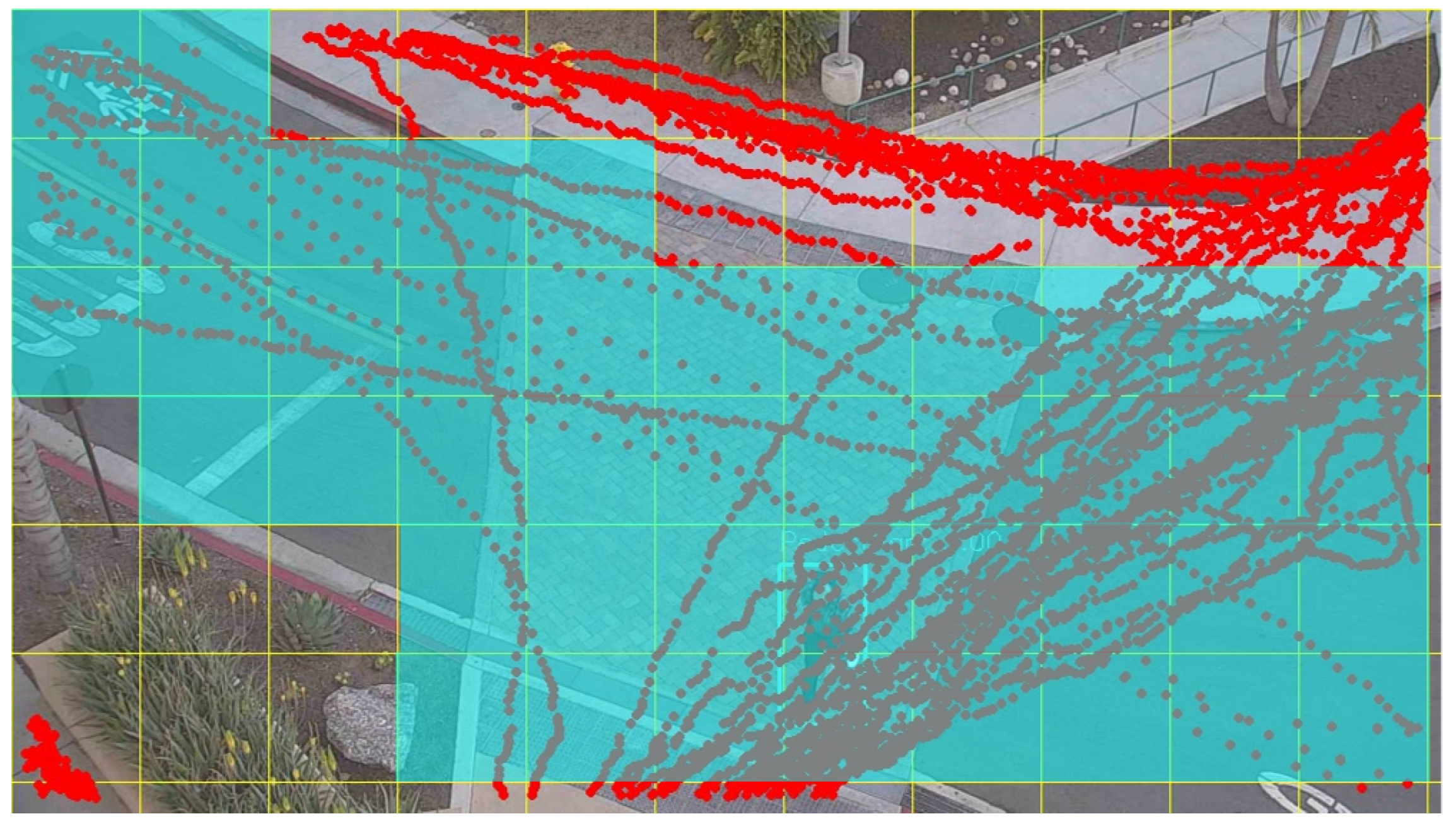
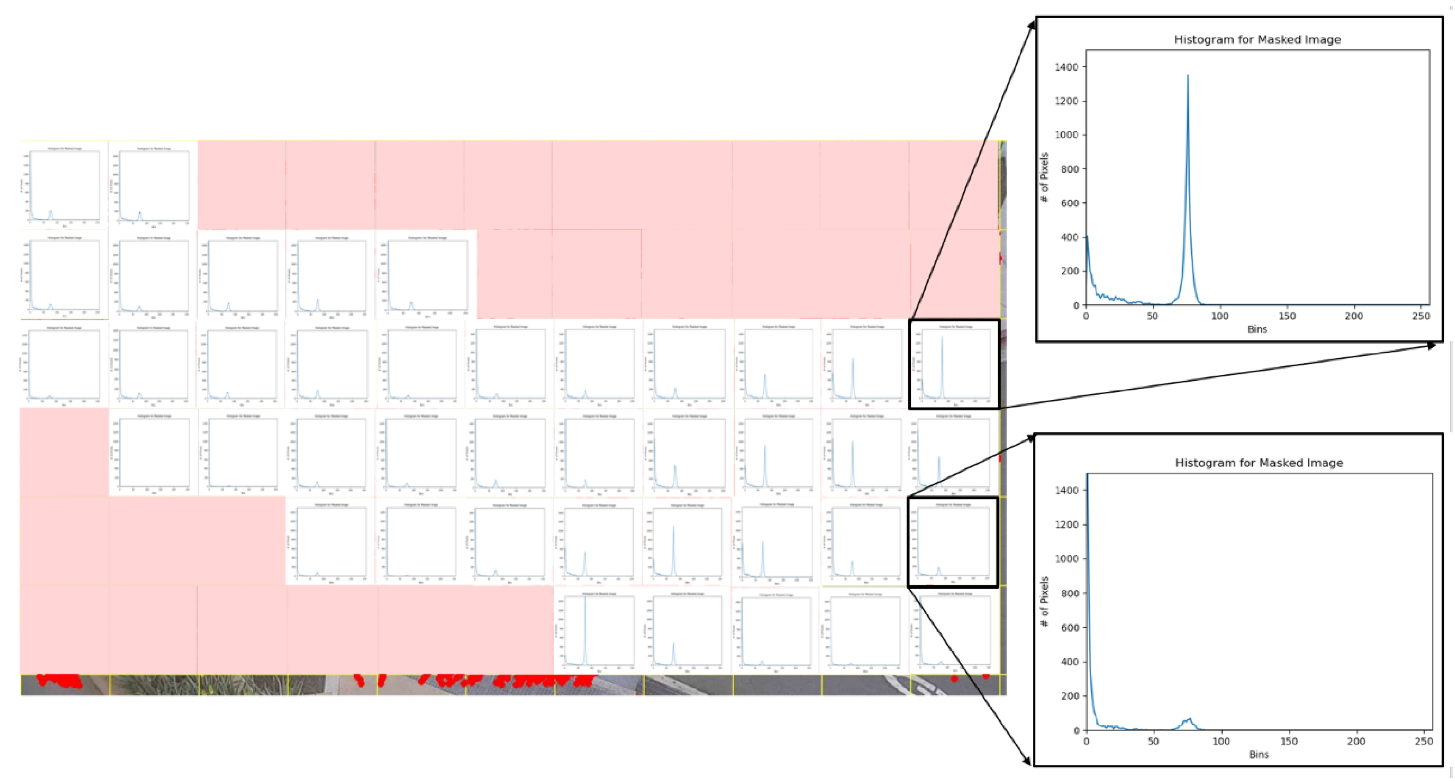
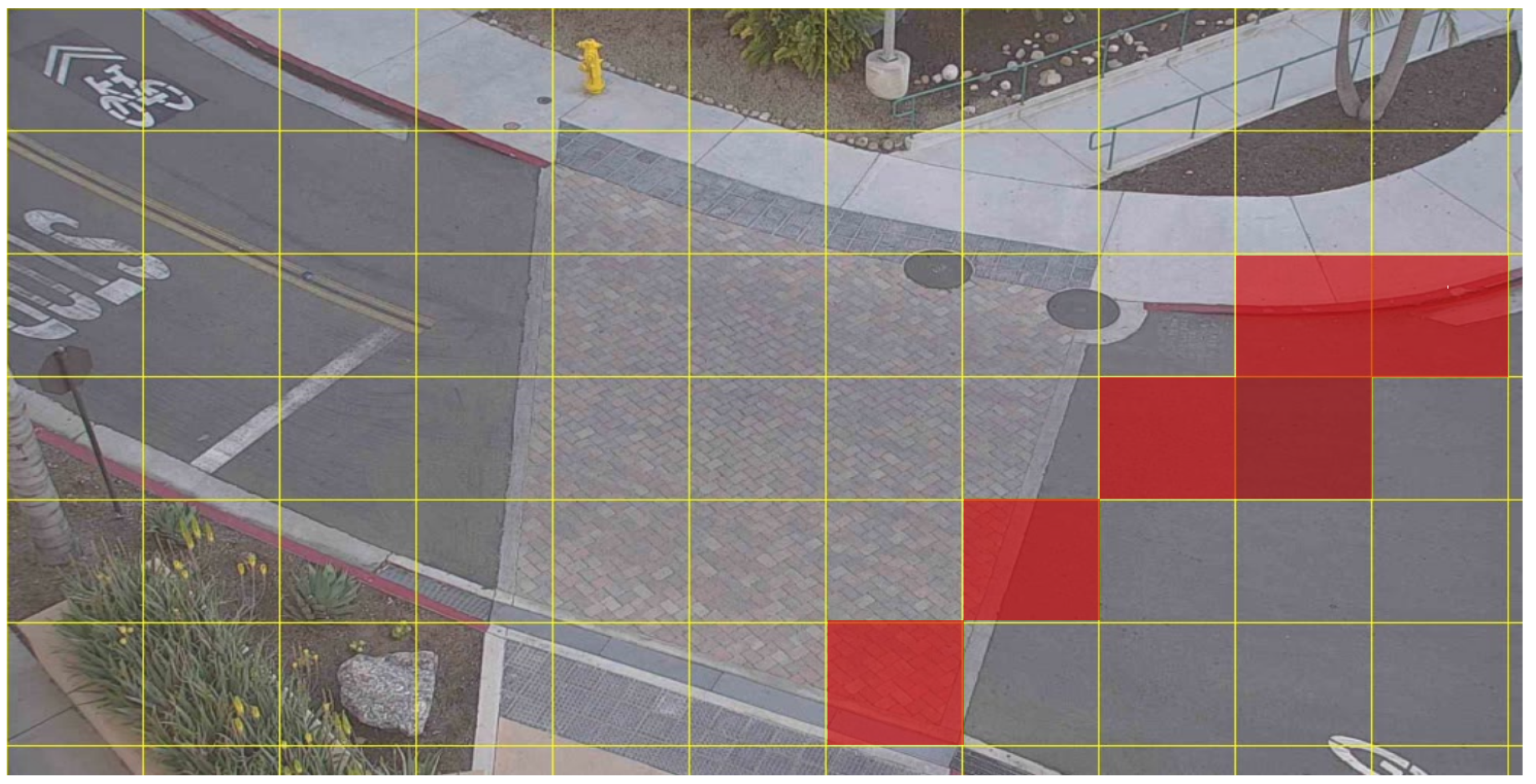
To determine a conflict zone, we calculate the center of a detected object’s bounding box and draw contrails. This can be seen in Figure 29, where only moving pedestrians are detected and their trajectories captured by the contrails in red. There is a minivan in the image that has not been detected and, therefore, will not leave any contrails, unlike the Lucas–Kanade Algorithm that leaves contrails for any object passing in front of the camera. This isolates the movement of the pedestrian and the skateboarders. Similarly, Figure 30 shows a skateboarder leaving contrails. Figure 31 demonstrates the condition after video is captured for a certain period of time. Our objective is to use these contrails to analyze areas with the densest streamlines, as this marks the areas where there was greatest pedestrian–skateboarder interaction. To accomplish this, the image is split into different grids. The grid with the greatest streamline density will then be marked as the hazardous region. For even finer granularity of the hazardous zones, the grid resolution can be reduced further. After generating contrails on an image, we remove the background image and have the contrails separated for analysis, as shown in Figure 32. However, specific grids are eliminated as they do not capture significant pedestrian-skateboard interaction. For example, the sidewalks only contain contrails of pedestrians only and have no impact on the pedestrian–skateboarder interaction. The grid region selected for analysis can be seen in Figure 33 marked in cyan. The masked image is then converted to a gray-scale image, and a histogram is computed for every selected grid. This can be seen in Figure 34, which also shows two cases where a grid yields a high peak representing a high density of streamlines and the other with a low peak, which indicates lower streamline density. After repeating this procedure for all the grids and choosing an appropriate threshold, the hazardous zones are selected, as shown in Figure 35, marked in red. This procedure can be made dynamic in real-time where, after time t, a snapshot will be taken, and the whole process will be repeated, updating the unstable region. For finer granularity and more robust hazardous region detection, the grid resolution can be refined. Since our goal is to identify and update hazardous regions in real-time, the SSDV1lite model seems to be the appropriate model to be used in this scenario, as the objective is the drawing of contrails and not classification accuracy. Moreover, the SSDV1lite model’s fast frame rate capability supports our real-time objective.

8. Conclusions

In this work we evaluated three object detection and classification models to classify pedestrians and skateboarders with the goal of developing in situ (“on device”) systems to increase the safety of skateboarder–pedestrian interaction. We leveraged state of the art deep learning architectures to enable two separate tasks. First, we automated the calculation of post encroachment time (PET), a Surrogate Safety Measure (SSM) and second, we performed real-time hazardous conflict zone determination of skateboarder–pedestrian interaction. We trained three separate object detection models and analyzed their advantages and weaknesses. We chose two suitable models for the two separate objectives and developed a new framework. The system we developed can be implemented on low-power ML inferencing devices, such as the Google Coral Edge TPU, and deployed on intersection light posts adjacent to existing video cameras. We have made our skateboarder and pedestrian conflict zone detection data set publicly available from the Center for Open Science data repository [47].
The deep-learning models evaluated in this study were trained on images captured and manually annotated from a live Real Time Streaming Protocol (RTSP) video stream transmitted from a camera located on the 6th story balcony of the Geology, Math, and Computer Science (GMCS) building on the campus of San Diego State University (SDSU). The camera was oriented to monitor a three-way intersection with a high frequency of automobile, bicycle, electric scooter, skateboard, and pedestrian traffic. Some limitations of this study include
  • The perspective of the camera used in this study was not equivalent to the perspective of a surveillance camera mounted on a traffic mast. Cameras affixed to traffic masts directly face oncoming traffic. Therefore, the images of pedestrians and skateboarders captured in this study are taken at different pan ( θ ), tilt ( ϕ ), and zoom (r) values than the spherical ( θ , ϕ , r ) coordinate configuration of a camera mounted on the mast at a city intersection.
  • The confidence scores of our models were higher when detecting objects in images containing no shadows. Pedestrians and skateboarders on overcast days or during illuminated nighttime periods had a higher chance of being detected and properly classified.
The current prototype performs well during overcast conditions when there is minimal shadow. For the model to perform well throughout the day, a real-time shadow removal algorithm must be implemented to extract shadows from the RTSP stream. Future efforts will involve developing algorithms for RTSP shadow removal, or implementing existing approaches presented in [48,49].
A total of 40 percent of vehicle collisions occur at intersections, and 20 percent of fatal collisions occur at intersections. Technologies that reduce the occurrence of intersection collisions are a transportation safety interest. Risk of vehicular collisions involving pedestrians and human-powered vehicles (HPVs), such as skateboards, at signalized intersections can be estimated using Surrogate Safety Measures (SSM). We have contributed to the development of a new framework for vehicle safety devices that can be installed on traffic lights to compute two SSMs, post encroachment time (PET) and time-to-collision (TTC), and the computational determination of hazard regions where conflicts can occur among pedestrians, HPVs, and motorized vehicles. An additional contribution of our work is a framework for measuring TTC using an object tracking model. SSMs in our new framework can be computed on small, low-power ASICs, such as the Google Coral Edge TPU, capable of performing ML inferencing through state-of-the-art mobile vision models such as MobileNet V2 at 400 FPS [40]. These devices can be installed adjacent to existing traffic intersection cameras. Real-time measurements can be input to intersection control instrumentation or safety and warning lights to alert drivers of a predicted collision prior to intersection encroachment. A conflict event is defined when the PET τ , for a threshold τ , typically 2 s. Detecting and recording the timestamp of conflict events at intersections between vehicles and HPVs can be used to train an artificial neural network (ANN) to make predictions when future conflict events are likely to occur. The trained ANN can be deployed in hardware to enable on-device inferencing, locally at intersections.

9. Future Work

In the future we propose to incorporate active stereoscopic infrared (IR) vision into our existing Pelco RGB-camera configuration. With two-dimensional (2D) RGB-only images of traffic intersections, accurate measurement of encroaching vehicle position, and thus velocity, is challenging. By adding an active stereo IR camera which projects a matrix of dots in the IR spectrum, distance to vehicles approaching an intersection can be estimated by measuring the displacement of the dots. The displacement field can then be superimposed on a 2D RGB image processed with the SSDV1lite model for vehicle and pedestrian detection and classification. Active IR stereo depth camera systems can achieve a depth accuracy absolute error within 2% at a maximum depth of 20 m. In addition, to achieve fine depth resolution within an intersection where vulnerable road users cross and are most at risk of collision, we propose to deploy LiDAR cameras, which provide accuracy within 14 mm at 9 m, on vertical light poles. Accurate estimation of depth will provide better measurement of PET and TTC, which depends on the computation of bounding-box centroid position in time during object-tracking.
Our current model computes a first-order average object velocity estimation to predict time to collision (TTC). For example, in Figure 36, the pixel displacement between subsequent frames of a detected object bounding-box centriod is shown in yellow. The frames shown were sampled at 9 frames/s. In the third frame, the value 6.57 has units of pixels/frame. We can estimate object velocity using the known height to pixel ratio of a reference object. The yellow fire hydrant is 4 feet tall and spans a height of 35 pixels in each frame, thus the detected skateboarder is estimated to be moving at a speed of
4 ft 35 px × 6.57 px frame × 9 frames s 6.76 ft s = 4.6 mph
Direction of travel relative to the frame is indicated by the angle of the superimposed green vector, rendered by OpenCV. We can use these velocity estimates to predict or evaluate the occurrence of potential crash events (e.g., between vehicles and pedestrians) in the region of an intersection, due to conflicting movements and interactions, and to use these computed analytics to proactively assess safety. Based on historical data captured by an on-board device we propose to develop, we aim to predict hazardous conditions from the state of an intersection as viewed by one or more cameras. These predictions can be used to design safer intersections by re-architecting traffic flow patterns and signaling algorithms. In addition, we propose to place LiDAR cameras directed toward, and focused on, shared-use paths that pedestrians, skateboards, and cyclists use to cross at an intersection. Because vehicle passengers, pedestrians and bicyclists are at risk of being seriously injured in accidents at intersections within the roadway crossing area, capturing real-time 3D position measurements at the mm scale of objects traversing a crossing area using LiDAR will provide greater accuracy in TTC estimations for collisions predicted to occur inside the crossing area. Measurements from the three (RGB, stereo IR, and LiDAR) camera systems will be fused, and the combined measurements will be used by an on-board device to estimate and report PET and TTC in real-time. Introducing active IR stereo into the traffic safety infrastructure has several advantages, including accurate measurement in outdoor environments under variable lighting conditions without requiring custom operator calibration. Our existing Pelco Esprit® traffic camera, which monitors a three-way intersection on the campus of San Diego State University (SDSU), is enclosed within an environmentally protective water-tight case and features a remote-control wiper blade to remove dust, dirt, and residue from a glass screen to prevent camera lens obstruction. We will design and fabricate a similar environmentally protective water-tight case for our stereo IR and LiDAR camera systems, so these cameras can be used in harsh weather conditions. At SDSU, we have access to a 3D printing machine that uses resins that form water-tight plastics. A prototype stereo IR and LiDAR system will be developed at SDSU and installed on campus next to our existing Pelco Esprit® traffic camera. Safety measurements and video will be streamed back to a nine-screen video wall at SDSU for evaluation. Probability of collision varies among traffic intersections, with some intersections designated as hazardous with a high Pedestrian Danger Index (PDI). For example, the fourth most dangerous intersection in San Diego is 4Th Av. and C St. in Chula Vista, with a PDI of 53 and a history of multiple pedestrian fatalities. To improve the safety of such hazardous locations, we propose to develop a prototype, to be mounted on a traffic light beam, containing an IR stereo depth camera, a LiDAR camera, and a hardware accelerator capable of in situ vehicle and pedestrian detection, classification, tracking, and TTC estimation.

Author Contributions

Conceptualization, C.E.S., A.J. and C.P.; methodology, C.E.S. and C.P.; software, C.E.S. and C.P.; validation, C.E.S., M.S., A.J. and C.P.; formal analysis, C.E.S., M.S. and C.P.; investigation, C.E.S. and C.P.; resources, A.J. and C.P.; data curation, C.E.S. and C.P.; writing—original draft preparation, C.E.S. and C.P.; writing—review and editing, M.S. and C.P.; visualization, C.E.S.; supervision, C.P.; project administration, C.P.; funding acquisition, A.J. All authors have read and agreed to the published version of the manuscript.

Funding

This research was funded by the United States Department of Transportation under grant number 04-110, Developing an Intelligent Transportation Management Center (ITMC) with a Safety Evaluation Focus for Smart Cities.

Institutional Review Board Statement

Not applicable.

Informed Consent Statement

Not applicable.

Data Availability Statement

Skateboarder and pedestrian conflict zone detection data supporting reported results can be found via URLs http://dx.doi.org/10.17605/OSF.IO/NYHF7, accessed on 25 August 2021, and http://dx.doi.org/10.17605/OSF.IO/CQD9Z, accessed on 25 August 2021.

Conflicts of Interest

The authors declare no conflict of interest. The funders had no role in the design of the study; in the collection, analyses, or interpretation of data; in the writing of the manuscript, or in the decision to publish the results.

Abbreviations

The following abbreviations are used in this manuscript:
MDPIMultidisciplinary Digital Publishing Institute
DOAJDirectory of open access journals
TLAThree letter acronym
LDLinear dichroism

References

  1. IOC Approves Five New Sports for Olympic Games Tokyo 2020. Available online: https://olympics.com/ioc/news/ioc-approves-five-new-sports-for-olympic-games-tokyo-2020 (accessed on 24 August 2021).
  2. McKenzie, L.B.; Fletcher, E.; Nelson, N.G.; Roberts, K.J.; Klein, E.G. Epidemiology of skateboarding-related injuries sustained by children and adolescents 5–19 years of age and treated in US emergency departments: 1990 through 2008. Inj. Epidemiol. 2016, 3, 10. [Google Scholar] [CrossRef] [Green Version]
  3. Fountain, J.L.; Meyers, M.C. Skateboarding injuries. Sport. Med. 1996, 22, 360–366, ISSN 1179-2035. [Google Scholar] [CrossRef]
  4. Kyle, S.B.; Nance, M.L.; Rutherford, G.W.; Winston, F.K. Skateboard-associated injuries: Participation-based estimates and injury characteristics. J. Trauma 2002, 53, 686–690, ISSN 2163-0763. [Google Scholar] [CrossRef]
  5. Forsman, L.; Eriksson, A. Skateboarding injuries of today. Br. J. Sport. Med. 2001, 35, 325–328, ISSN 1473-0480. [Google Scholar] [CrossRef] [PubMed] [Green Version]
  6. Panda, N.; Majhi, S.K. How effective is the salp swarm algorithm in data classification. In Computational Intelligence in Pattern Recognition; Springer: Berlin/Heidelberg, Germany, 2020; pp. 579–588. ISBN 978-3-319-89628-1. [Google Scholar]
  7. Dulebenets, M.A. A novel memetic algorithm with a deterministic parameter control for efficient berth scheduling at marine container terminals. Marit. Bus. Rev. 2017, 2, 302–330, ISSN 2397-3757. [Google Scholar] [CrossRef] [Green Version]
  8. D’Angelo, G.; Pilla, R.; Tascini, C.; Rampone, S. A proposal for distinguishing between bacterial and viral meningitis using genetic programming and decision trees. Soft Comput. 2019, 23, 11775–11791, ISSN 1432-7643. [Google Scholar] [CrossRef]
  9. Liu, Z.Z.; Wang, Y.; Huang, P.Q. AnD: A many-objective evolutionary algorithm with angle-based selection and shift-based density estimation. Inf. Sci. 2020, 509, 400–419, ISSN 0020-0255. [Google Scholar] [CrossRef] [Green Version]
  10. Pasha, J.; Dulebenets, M.A.; Kavoosi, M.; Abioye, O.F.; Wang, H.; Guo, W. An optimization model and solution algorithms for the vehicle routing problem with a “factory-in-a-box”. IEEE Access 2020, 8, 134743–134763, ISSN 2169-3536. [Google Scholar] [CrossRef]
  11. Behbahani, H.; Nadimi, N. A Framework for Applying Surrogate Safety Measures for Sideswipe Conflicts. Int. J. Traffic Transp. Eng. 2015, 5, 371–383, ISSN 2217-544X. [Google Scholar] [CrossRef] [Green Version]
  12. Peesapati, L.N.; Hunter, M.P.; Rodgers, M.O. Evaluation of Postencroachment Time as Surrogate for Opposing Left-Turn Crashes. Transp. Res. Rec. 2013, 2386, 42–51. [Google Scholar] [CrossRef] [Green Version]
  13. Zheng, L.; Ismail, K.; Meng, X. Traffic conflict techniques for road safety analysis: Open questions and some insights. Can. J. Civ. Eng. 2014, 41, 633–641. [Google Scholar] [CrossRef]
  14. Ozbay, K.; Yang, H.; Bartin, B.; Mudigonda, S. Derivation and Validation of New Simulation-Based Surrogate Safety Measure. Transp. Res. Rec. 2008, 2083, 105–113. [Google Scholar] [CrossRef] [Green Version]
  15. Hayward, J.C. Near miss determination through use of a scale of danger. Highw. Res. Rec. 1972, 384, 24–34, ISSN 0073-2206. [Google Scholar]
  16. Saffarzadeh, M.; Nadimi, N.; Naseralavi, S.; Mamdoohi, A.R. A general formulation for time-to-collision safety indicator. Proc. Inst. Civ. Eng. Transp. 2013, 166, 294–304. [Google Scholar] [CrossRef]
  17. Peesapati, L.N.; Hunter, M.P.; Rodgers, M.O. Can post encroachment time substitute intersection characteristics in crash prediction models? J. Saf. Res. 2018, 66, 205–211. [Google Scholar] [CrossRef]
  18. Graw, M.; König, H.G. Fatal pedestrian—Bicycle collisions. Forensic Sci. Int. 2002, 126, 241–247, ISSN 0379-0738. [Google Scholar] [CrossRef]
  19. Tuckel, P.; Milczarski, W.; Maisel, R. Pedestrian injuries due to collisions with bicycles in New York and California. J. Saf. Res. 2014, 51, 7–13, ISSN 0022-4375. [Google Scholar] [CrossRef] [PubMed]
  20. Fontaine, H.; Gourlet, Y. Fatal pedestrian accidents in France: A typological analysis. Accid. Anal. Prev. 1997, 29, 303–312, ISSN 0001-4575. [Google Scholar] [CrossRef]
  21. Choueiri, E.M.; Lamm, R.; Choueiri, G.; Choueiri, B. Pedestrian accidents: A 15-year survey from the United States and Western Europe. ITE J. 1993, 63, 36–42, ISSN 0162-8178. [Google Scholar]
  22. Robi, J. The 10 Most Dangerous Pedestrian Intersections in San Diego County. Available online: https://www.neighborhoods.com/blog/the-10-most-dangerous-pedestrian-intersections-in-san-diego-county (accessed on 24 August 2021).
  23. Shourov, E.C.; Paolini, C. Laying the Groundwork for Automated Computation of Surrogate Safety Measures (SSM) for Skateboarders and Pedestrians using Artificial Intelligence. In Proceedings of the 2020 Third International Conference on Artificial Intelligence for Industries (AI4I), Irvine, CA, USA, 21–23 September 2020; pp. 19–22. [Google Scholar] [CrossRef]
  24. Dutta, A.; Zisserman, A. The VIA Annotation Software for Images, Audio and Video. In Proceedings of the 27th ACM International Conference on Multimedia, Nice, France, 21–25 October 2019; ACM: New York, NY, USA, 2019. ISBN 978-1-4503-6889-6. [Google Scholar] [CrossRef] [Green Version]
  25. Dutta, A.; Gupta, A.; Zissermann, A. VGG Image Annotator (VIA). 2016. Available online: https://www.robots.ox.ac.uk/~vgg/software/via/ (accessed on 25 August 2021).
  26. San Diego State University Internet of Things Laboratory (IoTLab). Available online: http://iotlab.sdsu.edu/ (accessed on 25 August 2021).
  27. Bappy, J.H.; Roy-Chowdhury, A.K. CNN based region proposals for efficient object detection. In Proceedings of the 2016 IEEE International Conference on Image Processing (ICIP), Phoenix, AZ, USA, 25–28 September 2016; pp. 3658–3662, ISSN 15224880. [Google Scholar]
  28. Purkait, P.; Zhao, C.; Zach, C. SPP-Net: Deep absolute pose regression with synthetic views. arXiv 2017, arXiv:1712.03452. ISSN 2331-8422. [Google Scholar]
  29. Girshick, R. Fast r-cnn. In Proceedings of the IEEE International Conference on Computer Vision, Santiago, Chile, 7–13 December 2015; pp. 1440–1448, ISBN 0-8186-7042-8. ISSN 1063-6919. [Google Scholar]
  30. Ren, S.; He, K.; Girshick, R.; Sun, J. Faster R-CNN: Towards Real-Time Object Detection with Region Proposal Networks. arXiv 2015, arXiv:1506.01497. [Google Scholar] [CrossRef] [PubMed] [Green Version]
  31. He, K.; Gkioxari, G.; Dollár, P.; Girshick, R. Mask r-cnn. In Proceedings of the IEEE International Conference on Computer Vision, Venice, Italy, 22–29 October 2017; pp. 2961–2969, ISSN 1063-6919. [Google Scholar]
  32. Lin, T.Y.; Dollár, P.; Girshick, R.; He, K.; Hariharan, B.; Belongie, S. Feature pyramid networks for object detection. In Proceedings of the IEEE Conference on Computer Vision and Pattern Recognition, Honolulu, HI, USA, 21–26 July 2017; pp. 2117–2125, ISSN 1063-6919. [Google Scholar]
  33. Pramanik, A.; Pal, S.K.; Maiti, J.; Mitra, P. Granulated RCNN and multi-class deep sort for multi-object detection and tracking. IEEE Trans. Emerg. Top. Comput. Intell. 2021, 1–11, ISSN 2471-285X. [Google Scholar] [CrossRef]
  34. Redmon, J.; Divvala, S.; Girshick, R.; Farhadi, A. You only look once: Unified, real-time object detection. In Proceedings of the IEEE Conference on Computer Vision and Pattern Recognition, Las Vegas, NV, USA, 27–30 June 2016; pp. 779–788, ISSN 1063-6919. [Google Scholar]
  35. Liu, W.; Anguelov, D.; Erhan, D.; Szegedy, C.; Reed, S.; Fu, C.Y.; Berg, A.C. SSD: Single shot multibox detector. In Proceedings of the European Conference on Computer Vision, Amsterdam, The Netherlands, 8–16 October 2016; Springer: Berlin/Heidelberg, Germany, 2016; pp. 21–37, ISBN 978-3-319-46448-0. [Google Scholar]
  36. Li, Y.; Ren, F. Light-weight retinanet for object detection. arXiv 2019, arXiv:1905.10011. ISSN 2331-8422. [Google Scholar]
  37. Redmon, J.; Farhadi, A. Yolov3: An incremental improvement. arXiv 2018, arXiv:1804.02767. ISSN 2331-8422. [Google Scholar]
  38. Bochkovskiy, A.; Wang, C.Y.; Liao, H.Y.M. Yolov4: Optimal speed and accuracy of object detection. arXiv 2020, arXiv:2004.10934. ISSN 2331-8422. [Google Scholar]
  39. Wang, C.Y.; Yeh, I.H.; Liao, H.Y.M. You Only Learn One Representation: Unified Network for Multiple Tasks. arXiv 2021, arXiv:2105.04206. ISSN 2331-8422. [Google Scholar]
  40. Coral EdgeTPU Dev Board: A Development Board to Quickly Prototype on-Device ML Products. Available online: https://coral.ai/products/dev-board/ (accessed on 24 August 2021).
  41. Abadi, M.; Barham, P.; Chen, J.; Chen, Z.; Davis, A.; Dean, J.; Devin, M.; Ghemawat, S.; Irving, G.; Isard, M.; et al. Tensorflow: A system for large-scale machine learning. In Proceedings of the 12th USENIX Symposium on Operating Systems Design and Implementation (OSDI 16), Savannah, GA, USA, 2–4 November 2016; pp. 265–283, ISBN 978-1-880446-39-3. [Google Scholar]
  42. Rezatofighi, H.; Tsoi, N.; Gwak, J.; Sadeghian, A.; Reid, I.; Savarese, S. Generalized intersection over union: A metric and a loss for bounding box regression. In Proceedings of the IEEE Conference on Computer Vision and Pattern Recognition, Long Beach, CA, USA, 15–20 June 2019; pp. 658–666, ISBN 0-8186-7822-4. [Google Scholar]
  43. Henderson, P.; Ferrari, V. End-to-end training of object class detectors for mean average precision. In Proceedings of the Asian Conference on Computer Vision, Taipei, Taiwan, 20–24 November 2016; Springer: Berlin/Heidelberg, Germany, 2016; pp. 198–213, ISBN 978-3-030-69525-5. [Google Scholar]
  44. Rakshit, S. Intersection Over Union. Available online: https://medium.com/koderunners/intersection-over-union-516a3950269c (accessed on 24 August 2021).
  45. Rockikz, A. How to Perform YOLO Object Detection using OpenCV and PyTorch in Python. Available online: https://www.thepythoncode.com/article/yolo-object-detection-with-opencv-and-pytorch-in-python (accessed on 24 August 2021).
  46. Gettman, D.; Head, L. Surrogate safety measures from traffic simulation models. Transp. Res. Rec. 2003, 1840, 104–115. [Google Scholar] [CrossRef] [Green Version]
  47. Shourov, C.E.; Paolini, C. Skateboarder and Pedestrian Conflict Zone Detection Dataset. Available online: http://dx.doi.org/10.17605/OSF.IO/NYHF7 (accessed on 24 August 2021).
  48. Wang, Y. Real-time moving vehicle detection with cast shadow removal in video based on conditional random field. IEEE Trans. Circuits Syst. Video Technol. 2009, 19, 437–441, ISSN 1558-2205. [Google Scholar] [CrossRef]
  49. Jung, C.R. Efficient background subtraction and shadow removal for monochromatic video sequences. IEEE Trans. Multimed. 2009, 11, 571–577, ISSN 1941-0077. [Google Scholar] [CrossRef]
Figure 1. (a) Initial grid of feature points, (b) vehicle streamlines generated with OpenCV optical flow using the Lucas–Kanade estimation method, (c) superimposed artificially created conflict zone covering the area of greatest streamline number density, (d) vehicle being tracked, (e) vehicle centroid entering conflict zone at time 22:08:52.516, (f) vehicle centroid exiting conflict zone at time 22:08:52.956, (g,h) closer view showing conflict zone computed ingress and egress timestamps. Computed vehicle conflict zone residence time Δ t = 956 ms − 516 ms = 440 ms.
Futuretransp 01 00022 g001
Figure 2. Pelco Esprit® Enhanced Series camera.
Futuretransp 01 00022 g002
Figure 3. Region of Interest for Conflict Zone Analysis and Automated Computation of PET at San Diego State University.
Futuretransp 01 00022 g003
Figure 4. Images were obtained from eighteen different camera perspectives configured with different pan, tilt, and zoom values, shown in Table 1. Six selected perspectives are shown in sub-figures (af).
Futuretransp 01 00022 g004
Figure 5. Total number of annotations of skateboarders and pedestrians. All ground truth areas in images were hand-annotated using the VGG Annotator in the San Diego State University Internet of Things Laboratory [26].
Futuretransp 01 00022 g005
Figure 6. Image data according to time of the day. Only evening images were used, as a proof of concept, since morning and mid-day images contain shadows which impede the performance of the object detection model. A fast shadow removal algorithm can be used to remove shadows before feeding to a deep learning model.
Futuretransp 01 00022 g006
Figure 7. Ground Truth (red) v. Detection (blue) of a cat [44]. ©2019 Soumik Rakshit.
Futuretransp 01 00022 g007
Figure 8. Intersection over Union [45].
Futuretransp 01 00022 g008
Figure 9. The Faster R-CNN model stabilizes at an mAP above 99.5% at 0.5 IoU and oscillates above 98% at 0.75 IoU by the end of the training period.
Futuretransp 01 00022 g009
Figure 10. SSDV2 reaches a mAP of 98% at 0.5 IoU and oscillates around 92% at 0.75 IoU.
Futuretransp 01 00022 g010
Figure 11. The SSDV1lite model settles a little under 99.5% at 0.5 IoU and 97% at 0.75 IoU.
Futuretransp 01 00022 g011
Figure 12. The training loss for the Faster R-CNN model starts low and then decreases to nearly 0.00.
Futuretransp 01 00022 g012
Figure 13. The evaluation loss is around 0.1 for Faster R-CNN. There is clearly no over-fitting as the training loss and the evaluation loss values are close.
Futuretransp 01 00022 g013
Figure 14. The training loss of the SSDV2 model by the end of 200,000 steps is slightly above 1.00.
Futuretransp 01 00022 g014
Figure 15. The evaluation loss of SSDV2 by the end of the training is around 1.80. Again, both values being in the neighborhood of each other states no over-fitting in the model.
Futuretransp 01 00022 g015
Figure 16. The SSDV1lite model has a training loss of around 0.13.
Futuretransp 01 00022 g016
Figure 17. The SSDV1Lite model has an evaluation loss of around 0.2. This model also does not have an over-fitting problem.
Futuretransp 01 00022 g017
Figure 18. Faster R-CNN predicts the three objects correctly in the image (one skateboarder and two pedestrians) with confidence of 99% for all.
Futuretransp 01 00022 g018
Figure 19. The SSDV2 model evaluates the skateboarder as 99%, one pedestrian as 96%, and the other pedestrian as 99%.The image is pixelated due to its shrinkage from original shape to 300 × 300 . This was necessary because this particular model only takes an input dimension of shape 300 × 300 .
Futuretransp 01 00022 g019
Figure 20. The SSDV1lite model predicts the skateboarders with the confidence of 87% and the two pedestrians with the confidence of 81% and 80%.
Futuretransp 01 00022 g020
Figure 21. A pair of skateboarders entering and leaving a superimposed artificially created conflict zone shown in red one after another and their ingress and egress timestamps are recorded.
Futuretransp 01 00022 g021
Figure 22. The egress time for the first skateboarder occurs at 2:35:51.04. The ingress time of the following skateboarder occurs at 2:37:24.44.PET for this pair of entities is Δ t = 2:37:24.44 − 2:35:51.04 = 93.4 s.
Futuretransp 01 00022 g022
Figure 23. The grid area is reduced to solve the occlusion problem. In this figure, a skateboarder is misclassified as a pedestrian due to occlusion.
Futuretransp 01 00022 g023
Figure 24. Both skateboarders are correctly detected and registered inside the grid area with unique IDs.
Futuretransp 01 00022 g024
Figure 25. Skateboarder inside the grid has a registered ID. The skateboarder leaving the grid is de-registered. The pedestrian is yet to be registered, as she has not entered the grid area.
Futuretransp 01 00022 g025
Figure 26. Two pedestrians inside the grid with unique registered IDs.
Futuretransp 01 00022 g026
Figure 27. Automated collection of information for PET on the terminal.
Futuretransp 01 00022 g027
Figure 28. Data recorded on an Excel spreadsheet.
Futuretransp 01 00022 g028
Figure 29. Object detection model drawing contrails of pedestrians only.
Futuretransp 01 00022 g029
Figure 30. Object detection model drawing contrails of skateboarders only.
Futuretransp 01 00022 g030
Figure 31. Contrails of only pedestrians and skateboarders recorded after running on video for sometime.
Futuretransp 01 00022 g031
Figure 32. Contrails copied to a mask for analysis.
Futuretransp 01 00022 g032
Figure 33. Selected Grids to be analyzed.
Futuretransp 01 00022 g033
Figure 34. Histogram calculated for selected grids. This figure shows two cases where a grid cell yields a high peak representing a high density of streamlines, and another cell with a low peak indicating lower streamline density.
Futuretransp 01 00022 g034
Figure 35. Conflict zones determined after streamline density analysis. For finer granularity and more robust hazardous region detection, the grids can be made refined.
Futuretransp 01 00022 g035
Figure 36. First-order average object velocity estimation to predict time to collision (TTC). Units of numbers shown in yellow are pixels/frame.
Futuretransp 01 00022 g036
Table 1. Camera perspective configuration parameters.
PerspectivePan (Degrees)Tilt (Degrees)
184.211.04
284.21−0.55
385.71−3.49
485.71−5.26
592.23−8.05
697.79−22.78
7110.48−28.75
8122.28−33.62
9139.75−35.95
10174.22−36.54
11179.71−36.54
12234−36.54
13249.27−25.79
14245.85−25
15249.04−21.87
16255.57−10.74
17253.77−8.17
18255.97−5.6
Table 2. Elapsed time and fps tabulated.
ModelElapsed Timefps
Faster R-CNN0.08≈35
SSDV20.02≈54
SSDV1lite0.03≈102
Table 3. Summarized mean average precision at 0.5 IoU and 0.75 IoU, evaluation loss, and frames per second.
Model[email protected][email protected]Evaluation Lossfps
Faster R-CNN99.598.00.1≈35
SSDV29892.01.8≈54
SSDV1lite99.597.00.2≈102
Publisher’s Note: MDPI stays neutral with regard to jurisdictional claims in published maps and institutional affiliations.