Article

Comprehensive Assessment of CNN Sensitivity in Automated Microorganism Classification: Effects of Compression, Non-Uniform Scaling, and Data Augmentation

by
Dimitria Theophanis Boukouvalas
1,
Márcia Aparecida Silva Bissaco
2,
Humberto Dellê
3,
Alessandro Melo Deana
1,
Peterson Adriano Belan
1 and
Sidnei Alves de Araújo
1,*
1
Informatics and Knowledge Management Graduate Program, Nove de Julho University (UNINOVE), Vergueiro Street, 235/249, Liberdade, São Paulo, SP 01504-001, Brazil
2
Biomedical Engineering Graduate Program, Universidade de Mogi das Cruzes, Av. Dr. Cândido Xavier de Almeida e Souza, 200, Centro Cívico, Mogi das Cruzes, SP 08780-911, Brazil
3
Medicine Graduate Program, Nove de Julho University (UNINOVE), Vergueiro Street, 235/249, Liberdade, São Paulo, SP 01504-001, Brazil
*
Author to whom correspondence should be addressed.
BioMedInformatics 2025, 5(4), 61; https://doi.org/10.3390/biomedinformatics5040061
Submission received: 6 August 2025 / Revised: 13 September 2025 / Accepted: 10 October 2025 / Published: 31 October 2025

Abstract

Background: The growing demand for automated microorganism classification in the context of Laboratory 4.0 highlights the potential of convolutional neural networks (CNNs) for accurate and efficient image analysis. However, their effectiveness remains limited by the scarcity of large, labeled datasets. This study addresses a key gap in the literature by investigating how commonly used image preprocessing techniques, such as lossy compression, non-uniform scaling (typically applied to fit input images to CNN input layers), and data augmentation, affect the performance of CNNs in automated microorganism classification. Methods: Using two well-established CNN architectures, AlexNet and DenseNet-121, both frequently applied in biomedical image analysis, we conducted a series of computational experiments on a standardized dataset of high-resolution bacterial images. Results: Our results demonstrate under which conditions these preprocessing strategies degrade or improve CNN performance. Using the findings from this research to optimize hyperparameters and train the CNNs, we achieved classification accuracies of 98.61% with AlexNet and 99.82% with DenseNet-121, surpassing the performance reported in current state-of-the-art studies. Conclusions: This study advances laboratory digitalization by reducing data preparation effort, training time, and computational costs, while improving the accuracy of microorganism classification with deep learning. Its contributions also benefit broader biomedical fields such as automated diagnostics, digital pathology, clinical decision support, and point-of-care imaging.

Graphical Abstract

1. Introduction

Microorganisms are organisms that can only be seen under a microscope. Examples are viruses, bacteria, protozoa, unicellular algae, fungi (unicellular yeasts and multicellular fungi), and mites [1]. Among these, pathogenic microorganisms are of great interest and concern due to their impact on public health. For instance, COVID-19, caused by the SARS-CoV-2 virus, led to over 7 million deaths from the beginning of the pandemic in 2019 until April 2024 [2]. Non-pathogenic microorganisms are also significant in various industries, such as agribusiness and food, where they can either spoil food or beneficially transform it into products like bread, cheese, and wine. In pharmaceuticals, microorganisms are crucial for manufacturing antibiotics such as penicillin [1].
Correct identification and classification of microorganisms are critical for detecting and preventing disease outbreaks, tracking antibiotic resistance, and monitoring disease trends to assess the effectiveness of prevention measures. Traditionally, this classification is performed by specialists through the visual examination of microscopic images. However, manual processes, especially complex ones, have high error rates, prompting laboratories to invest in automating this task to improve accuracy, standardization, and speed.
Deep learning (DL) is a rapidly developing field for the classification of microorganisms [3]. Recent research includes the development of approaches for microscopic holographic screening of spores of Bacillus anthracis (anthrax) [4]; methods for classifying bacterial colonies to detect and classify the hemolysis effects [5]; and new DL techniques to enhance microorganism analysis by speeding up processes, reducing costs, and increasing the consistency and accuracy [6]. Advances in deep-network architectures, the availability of large computing power, and access to extensive training data have contributed to the successful use of DL in this field [7].
Convolutional neural networks (CNNs) are among the most prominent DL techniques in image pattern recognition, including cell and microorganism identification [8,9]. CNNs are advantageous because they learn image processing filters automatically, unlike conventional machine learning algorithms that require separate implementation of these filters to extract important features [10]. However, CNNs require large training datasets to achieve high generalization capacity, a significant challenge in biological and medical sciences due to the labor-intensive and time-consuming nature of acquiring well-annotated images [10,11,12,13,14,15].
Recent peer-reviewed studies reinforce the importance of CNNs in biomedical image analysis. Mienye et al. [16] provided a comprehensive review of CNN architectures, highlighting their impact on disease diagnosis, segmentation, and classification, while emphasizing ongoing challenges such as data scarcity, generalization, and computational cost. Wu et al. [17] conducted a comparative study on bacterial image classification using CNNs, including AlexNet and DenseNet-121, and demonstrated that DenseNet consistently outperformed other models in terms of accuracy and robustness. Schäfer et al. [18] further advanced the field by introducing UMedPT, a universal model pretrained on diverse biomedical images, which significantly outperformed ImageNet-based pretraining under limited-data conditions. Together, these works contextualize the present study, which explores the impact of preprocessing and data quality on CNN performance for microorganism classification, offering insights relevant to Laboratory 4.0 applications.
To address the lack of large datasets, techniques such as transfer learning and data augmentation are employed. Transfer learning uses pre-trained CNNs on general images and refines them with domain-specific images [14,19,20]. However, some studies, like that of Hay et al. [21] found no improvement in classification accuracy with this approach. Traditional data augmentation involves increasing the number of training examples through geometric transformations (rotating, scaling, mirroring, shearing, etc.), noise addition, and cropping, enhancing the model’s generalization ability.
Despite the benefits of data augmentation, some operations can negatively impact CNN training, especially given the high similarity between different microorganism images. Several studies have highlighted the limitations of traditional data augmentation schemes, particularly in scenarios that demand a deeper theoretical understanding of their effects [7,22]. This study investigates how rotation, mirroring, and cropping operations in data augmentation affect CNN learning, contributing to the proper expansion of small microorganism image datasets available in the literature.
When training CNNs, images are often scaled down and reshaped into square dimensions to meet input layer requirements and reduce computational costs; however, this process can lead to the loss of important visual information and negatively affect learning. This study also addresses the impact of non-uniform scaling on CNN performance; a problem not extensively covered in the literature.
Additionally, image compression, commonly used for storage and transfer, can affect image quality and subsequently CNN accuracy [23]. Main libraries used in the development of computer vision systems use qualities that vary from 75% (Pillow and Scikit-image) to 95% (OpenCV) as standard for JPEG (main compression format), which may lead to performance degradation. This study analyses how different levels of image compression (lossy or lossless) influence the performance of CNNs, specifically AlexNet [24] and DenseNet-121 [25], by referencing studies on compression’s impact on image classification [23,26,27].
The context discussed above leads to the identification of the following research gaps:
  • Image compression: reducing the amount of data needed to represent a digital image is widely used for data storage and communication. However, the influence of compression type (lossy or lossless) on CNN accuracy remains unexplored in microorganism classification.
  • Non-uniform scaling: adjusting image size to fit CNN input layers, often resulting in non-uniform scaling, may impact classification accuracy. However, studies investigating this influence are scarce.
  • Dataset size: while CNNs excel with large datasets, the impact of smaller datasets on classification accuracy, particularly in biological images, requires further exploration.
  • Data augmentation techniques: the influence of common data augmentation operations (e.g., rotation, mirroring, cropping) on CNN learning remains inadequately studied in microorganism classification.
Our study offers relevant contributions to the modeling and optimization of CNNs, particularly in scenarios involving limited biological image datasets. Through a simulation-based framework, we systematically examined how commonly used preprocessing practices influence CNN performance in microorganism classification. The main contributions of this work include:
  • A practical demonstration of how dataset size critically affects classification accuracy, reinforcing the importance of data volume in deep learning applications for microorganism recognition;
  • A detailed analysis of the effects of image compression and non-uniform scaling—procedures often used to adapt images to CNN input layers—on classification outcomes;
  • A systematic evaluation of data augmentation techniques, such as mirroring, rotation, and noise addition, identifying conditions under which they enhance or hinder model performance.

2. Related Work

Although various studies have addressed factors relevant to this study in different contexts, a comprehensive analysis of compression, non-uniform scaling, and data augmentation techniques in the context of microorganism classification using DL has been lacking in the literature from 2011 to July 2025. For instance, while Ref. [28] explored the impact of data augmentation on DL models using general-scope images, they did not delve into the specific effects of individual data augmentation techniques. Similarly, Ref. [7] provided insights into data augmentation methods but focused on broader applications such as classifying Canadian Institute for Advanced Research–CIFAR patterns.
Conventional machine learning techniques, including supervised methods like artificial neural networks, support vector machines, k-nearest neighbors, and decision trees; and the unsupervised methods like expectation-maximization, self-organizing maps, k-means, fuzzy c-means, and density-based clustering have shown efficacy in image analysis tasks [12]. The most used DL techniques include autoencoder neural networks, deep neural networks, deep belief networks, recurrent neural networks, Boltzmann restricted machines, and CNNs [11,29]. Among these, the CNNs have gained prominence in image pattern recognition due to their automatic feature recognition capabilities, making them well-suited for microorganism classification tasks [8].
In DL approaches, performance increases as the amount of data increases [3]. Training CNNs requires the use of large datasets (thousands of images). Despite the advantages of DL, the scarcity of annotated biological image datasets has hindered its widespread adoption [10,11,12,13].
To address dataset limitations, researchers have increasingly turned to data augmentation techniques to augment training data and enhance DL model performance [21,28,29,30,31,32,33,34,35,36,37].
The properties and design of the data augmentation method are critical in determining their impact on augmented images and in selecting the most suitable method for the task at hand [7]. Additionally, existing studies have highlighted certain limitations of data augmentation strategies, requiring a better theoretical understanding of data augmentation [20]. Therefore, it is essential to comprehend how each technique influences the performance of the chosen network for specific image types, such as those used in this study’s images. This understanding allows for more informed choices regarding the methods used. The future of data augmentation lies in hybridization, where different methods are combined to optimize accuracy or solve specific problems [7]. Additionally, the development of automated data augmentation solutions is increasing. For instance, the work presented by [38,39] introduces automated solutions that leverage studies on network performance using various. data augmentation techniques to select the more appropriate ones. Furthermore, some researchers have opted to use hybrid networks combining LeNet [40], one of the pioneering DL networks, with more advanced architectures such as AlexNet [24] and InceptionV3 [41]. This approach aims to leverage the strengths of each network to achieve superior classification results [20,42,43].
Another technique employed is the use of transfer learning with pre-trained CNNs. Studies by [19,20,44] utilized this approach employing CNNs such as AlexNet, GoogLeNet, and ResNet-101, pre-trained on general scope images, which do not address the specific challenges related to biological images. Only Ref. [21] applied transfer learning with pre-trained CNNs using biological images but did not demonstrate an improvement in classification accuracy.
Regarding the images used, there is a wide variety of biological sample preparations, such as Gram staining, as well as different microscopy methods, such as phase contrast and fluorescence [1]. Owing to this variety, research concentrates on certain methods commonly used in clinical analysis and on specific cells and microorganisms. The datasets in the literature vary on image type and research objective. Some authors use images of colony forming units [5,29]; images of sputum samples to identify tuberculosis [32,45], images obtained from different image datasets [20]; and images acquired for specific research [33,46,47,48,49,50].
Image compression, whether lossy or lossless, can significantly affect the performance of CNNs. For instance, in Ref. [27], researchers investigated the degradation caused by the compression of point cloud lifting and 3D surface generation from drone-acquired images. They compared TIFF (lossless compression) and JPEG (lossy compression) formats across various compression levels. Similarly, Ref. [26] evaluated the impact of image compression on CNN performance for classifying steel surface defects. Additionally, Ref. [23] proposed a compression-based data augmentation method to improve the CNN performance and model generalization, particularly for images with low compression quality. Notably, both studies also considered the JPEG format in their evaluations.
Currently, the use of DL is still incipient for microorganism image analysis. There is a great diversity of microorganisms and various ways to obtain images from them. Furthermore, several CNN architectures, different parameter compositions and different ways to enlarge training datasets can be used for developing solutions, suggesting that there is a vast field for research.
One challenge in microorganism classification lies in the inherent similarity between images of different microorganisms. Despite ongoing research efforts aimed at classification, which aids in expediting analysis and supports specialists in their daily workflows, there remains significant work to be done in tailoring CNNs and procuring adequate image datasets.

3. Materials and Methods

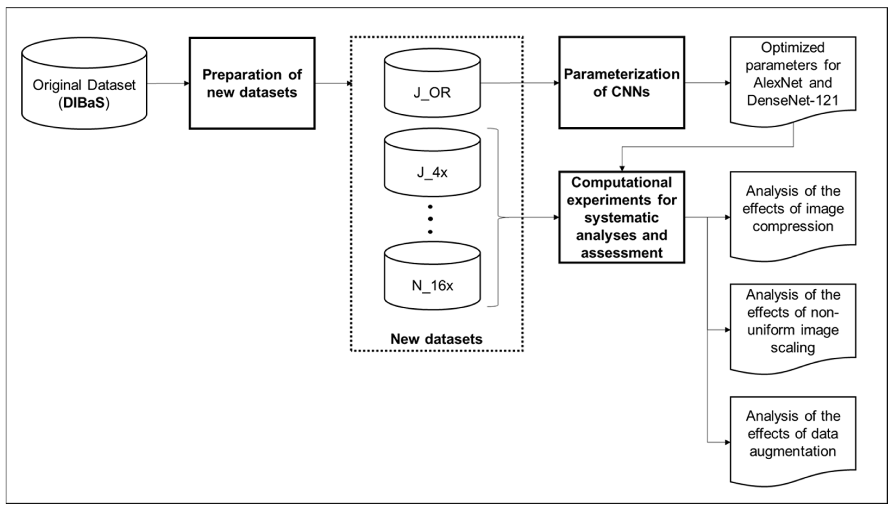
In this study, we adopted a simulation-driven methodology to systematically investigate how different image preprocessing factors affect the performance of convolutional neural networks (CNNs) in automated microorganism classification. Our approach, illustrated in Figure 1, was structured into the following key steps:
  • Preparation of new datasets: To conduct the computational experiments, new datasets were created based on the original dataset. This involved:
    • Creation of datasets for each experiment: Tailored datasets were created to analyze different factors influencing CNN performance.
    • Dataset splitting: The created datasets were divided into two parts: 80% for training and 20% for validation.
  • Parameterization of CNNs: The CNN models, AlexNet and DenseNet-121, were parameterized using the original dataset. This included the optimization of hyperparameters to enhance the performance of both CNN architectures: batch size, learning rate, and number of epochs were optimized.
  • Experiments for analyses and assessment: The experiments conducted for each analysis included training and validating using the created datasets and optimized hyperparameters. Training involved iteratively updating the model’s internal parameters over multiple epochs until convergence, while validating evaluated the model’s performance on unseen data. The experiments included:
    • Analysis of image compression: Evaluation of the impact of image compression (lossy and lossless) on CNN performance using datasets converted to different file extensions (JPG and PNG).
    • Analysis of non-uniform image scaling: Investigation of the influence of non-uniform image scaling on CNN performance using datasets resized to different dimensions.
    • Analysis of data augmentation operations: Evaluation of the effects of mirroring, rotation, and noise addition on CNN performance using datasets augmented with these techniques.
Figure 1. Steps of the proposed approach.
Biomedinformatics 05 00061 g001

3.1. Rationale for Experimental Design

The methodology choices were driven by the need to optimize CNN performance for microorganism classification while addressing limitations in data availability. We selected AlexNet and DenseNet-121 due to their effectiveness in biological image classification tasks, as reported in the literature. Parameterization involved tuning hyperparameters to optimize CNN training, while normalization ensured standardized input data for improved training stability. Dataset splitting enabled unbiased evaluation of CNN performance. These choices were made to align the methodology with the study objectives and maximize the insights gained from the experimental analysis.
There are several CNN architectures, many of which were developed focusing on the classification of the image set provided by the ImageNet Project [24], which contains more than 14 million images distributed in 100 classes. The AlexNet is one of the earliest developed CNNs. It has 60 million parameters and obtained an accuracy of 63.3% in the ImageNet classification. Although its results are considered low compared to other more recent architectures such as the DenseNet-121, the results presented in works found in the literature for the classification of microorganisms, such as those related by [19,20,42,50,51,52,53], were expressive, reaching an accuracy of 96.63% for cell classification in the work of [20], and 97.24% for microorganism classification in the work of [54], while the DenseNet-121 architecture, tested by [52], obtained an accuracy of 98.65% for the classification of white blood cells.
The AlexNet is an architecture considerably tested in the researched literature and serves as a comparison parameter in the present research, whereas the DenseNet-121 was tested in only one work; however, it is a viable option owing to the use of few computational resources aided by good accuracy results. The fundamental differences between the two architectures are that the AlexNet uses less computational resources (between 55 and 60 G-FLOPs), performs fewer convolutions (5), and has more parameters (56,455,969), whereas the DenseNet-121 uses more computational resources (between 75 and 80 G-FLOPs), performs more convolutions (120), and has a smaller number of parameters (7,071,329). An exclusive feature of the DenseNet-121 is the use of direct connections between each layer and the other layers, called dense layers.
In the selection of non-uniform scaling, a crucial consideration stemmed from the architectural specifications of the chosen CNNs, AlexNet, and DenseNet-121. The input layer requirements for these models necessitate square images, whereas our original microorganism images exhibit rectangular dimensions of 2048 × 1532 pixels. Consequently, to align with the input layer specifications, non-uniform scaling was imperative. Specifically, we resized AlexNet input images to 227 × 227 pixels and those for DenseNet-121 to 224 × 224 pixels. This resizing process inevitably introduces distortion due to the discrepancy in aspect ratios between the original and scaled images.
Expanding on our approach to data compression, we implemented lossy compression at varying levels (50%, 75% and 95%) to simulate different degrees of image degradation. This approach allows us to mimic real-world scenarios where image quality may be compromised due to compression during storage or transfer. We specifically chose these compression levels to align with common practices in computer vision development, where libraries like Pillow and Scikit-image typically default to 75% compression quality, while OpenCV often employs 95%.
In our experiments, the percentages (50%, 75%, and 95%) correspond directly to the JPEG quality factor used during image conversion. This definition ensures reproducibility, as the quality factor is a standard parameter in widely used image-processing libraries. While file size reductions vary depending on image content, the quality factor provides a consistent and interpretable measure of compression strength.
The choice of data augmentation techniques was based on their effectiveness ©n enhancing CNN performance while addressing specific challenges in microorganism classification. Cropping allows the model to learn robust features by focusing on relevant regions of the image, mirroring diversifies the training dataset without increasing data collection efforts, rotation helps the model generalize better to unseen orientations of microorganisms, and noise addition increases the model’s robustness to variations in image quality.
In our comparative analysis approach, we qualitatively assessed the impact of different experimental factors on CNN performance based on metrics such as accuracy. To analyze the results comprehensively, we employed boxplots due to their ability to represent data distribution effectively, including measures of central tendency, variability, and potential outliers. By utilizing boxplots, we aimed to provide a clear and concise depiction of the performance variations across different experimental conditions and factors influencing CNN performance.

3.2. Image Dataset

The images used in this study are sourced from the Digital Images of Bacteria Species dataset (DIBaS), curated by (Zieliński et al. 2017 [50]) and available at https://doctoral.matinf.uj.edu.pl/database/dibas/ (accessed on 13 February 2022; no longer available; Now it is mirrored in https://github.com/gallardorafael/DIBaS-Dataset?utm_source=chatgpt.com (accessed on 5 August 2025)). These images were captured using an Olympus CX31 Upright Biological Microscope equipped with an SC30 camera (Olympus, Tokyo, Japan) and a Nikon50 objective (Nikon, Tokyo, Japan) under oil immersion at 100× magnification. All samples underwent Gramm staining. The DIBaS dataset comprises 689 high-quality images of 33 bacterial species with dimensions of 1532 × 2048 pixels. The dataset contains between 20 and 23 images per species, resulting in a slightly imbalanced class distribution. Table 1 lists the species and number of images in the dataset.
Among the datasets sourced from the literature, the DIBaS dataset offers standardized images of bacteria, distinguishing it from other datasets. The primary motivation for utilizing the DIBaS dataset in our experiments was its standardized nature. The standardized images of DIBas, as illustrated in Figure 2a, facilitate microorganism classification without being influenced by the acquisition process. As shown in Figure 2, standardized images, such as Figure 2a, enable classification based on morphological differences among microorganisms. However, when images are obtained from different sources (e.g., Figure 2b,c), variations in background, magnification, ambient lighting, and other factors can introduce distinct patterns for classification, regardless of microorganism morphology. It should be noted that in a laboratory environment, images intended for analysis are typically standardized.

3.3. Preparation of New Datasets

To conduct the computational experiments, we created new datasets (which are described in Table A1 in Appendix A using the original DIBaS dataset as a base. The reasons for creating such datasets are explained below.
In the DIBaS dataset, images have dimensions of 1532 × 2048 pixels, larger than those used for input in the first layer of the CNNs AlexNet and DenseNet-121, which receive images of 227 × 227 and 224 × 224 pixels, respectively. This allows the creation of datasets of cropped images from the original images (OR) as a means of data augmentation.
Note that the DIBaS dataset comprises images in the TIF file extension (high resolution, lossless compression), which is not supported by the considered CNNs. Thus, images were first converted to the supported extensions (JPG and PNG), further allowing the evaluation of the influence of image quality after compression (lossy and lossless).
Following, datasets were created to analyze the influence of non-uniform image scaling using the DIBaS dataset images converted to PNG or JPG. Finally, to analyze the techniques of mirroring, rotation, and noise addition, datasets were created using the OR dataset converted to PNG (lossless compression).
The datasets were named to briefly represent the type of experiment conducted with images. Thus, the datasets whose names start with the letter “J” are composed of the original images converted to JPG; “J50”, J”75” and “J95” refer to image quality after compressions, that is, 50%, 75%, and 95%. The datasets starting with the letter “P” comprise the original images converted to PNG (lossless compression). The datasets starting with the letter “S” comprise cropped images with dimensions 227 × 227 (required by AlexNet) or 224 × 224 (required by DenseNet-121). The following datasets use the original images converted to PNG and apply specific data augmentation techniques. Thus, the datasets starting with the letter D contain images cropped into squares (using the largest possible dimension of the original image); M represents the datasets for which mirror was applied; R represents the datasets for which the 90, 180 and 270-degree rotations were applied; A represents the datasets for which random rotations at angles between 0 and 90 degrees were applied; and N represents the datasets to which the gaussian, salt and pepper, and Poisson noise were added.
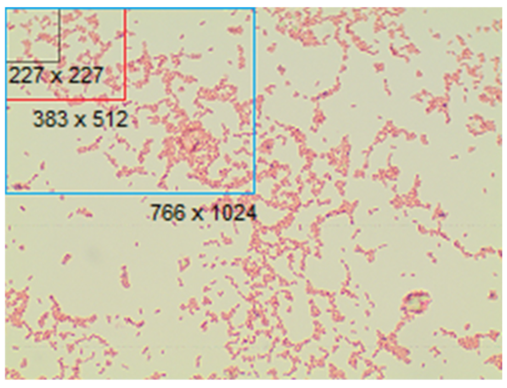
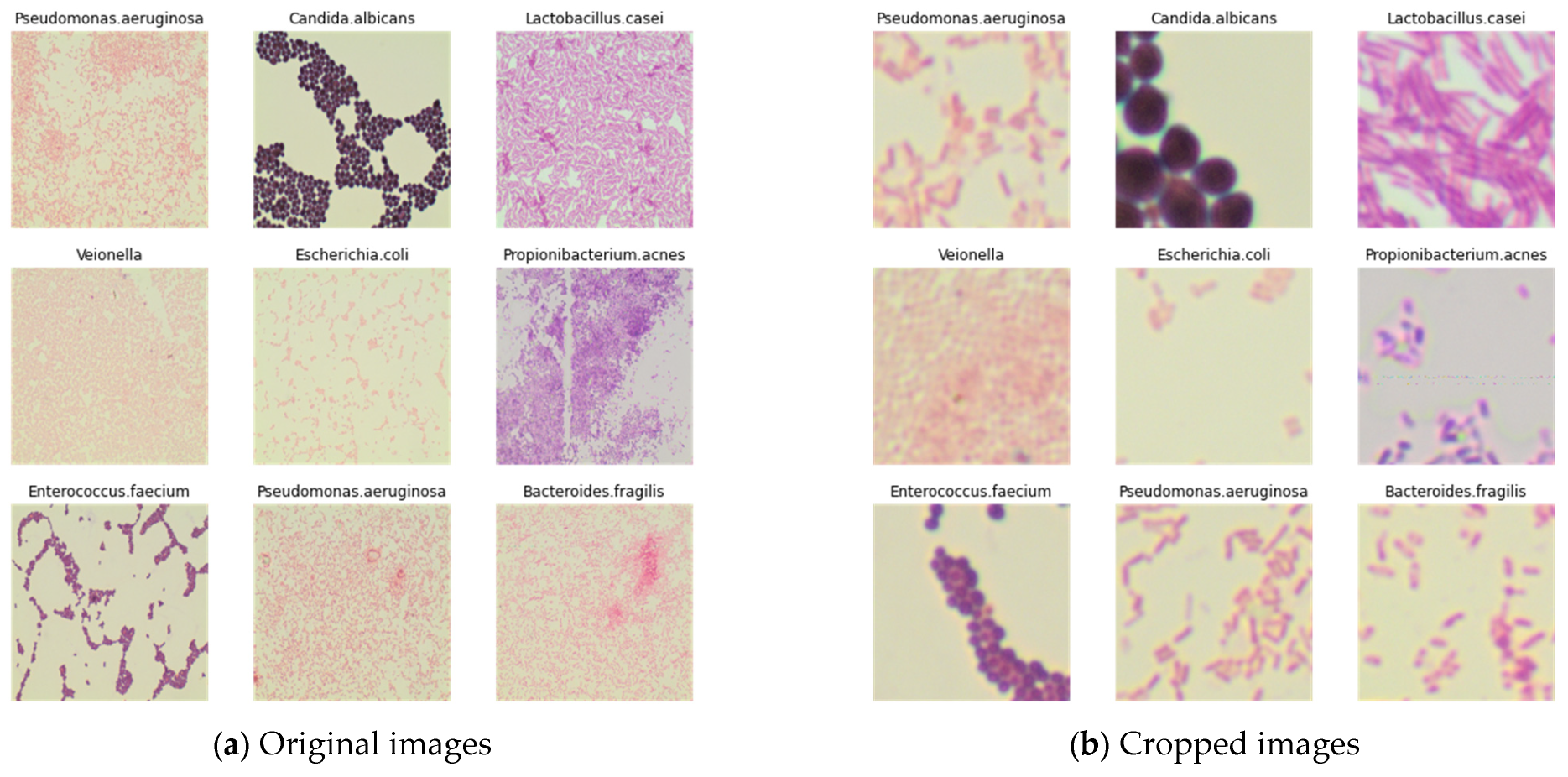
Image cropping is widely used for data augmentation and is usually performed by randomly cropping pieces of the image or by cropping the image into equal parts so as not to lose or repeat any information. Figure 3 shows examples of cropping used in this study.
During the training of AlexNet and DenseNet-121, images are resized to 227 × 227 and 224 × 224 pixels. Thus, by maintaining the same ratio between images on the different datasets, we guarantee that the same deformation occurs due to non-uniform scaling, whose influence is analyzed in Section 4.3. The pre-processing of images aims at their standardization before input to the CNN’s algorithm. This includes normalizing by applying the mean of the color channels and standard deviation and converting the pixel values to the interval [0.1]. No post hoc filtering was applied to the automatically generated crops; all samples—including occasional blank or low-information tiles—were retained to avoid selection bias and ensure reproducibility. Finally, in each experiment the image datasets were divided into two parts: 80% for training and 20% for validation, and to reduce bias and improve reliability, the dataset was randomized before splitting. Experiments were also repeated with different random seeds, which yielded consistent results across runs.

3.4. Parameterization of CNNs

The selection of appropriate hyperparameters and variables plays a crucial role in training neural networks, impacting model performance and convergence. In this section, we detail the rationale behind variable selection, including preliminary experiments and hyperparameter tuning, to optimize the training of our convolutional neural network (CNN) models. In this study, AlexNet and DenseNet-121 were initialized with random weights and trained entirely on the DIBaS dataset. No transfer learning or pretraining with ImageNet (or other datasets) was applied, ensuring that all results reflect training exclusively on microorganism images.
To gain insights into the behavior of our chosen CNN architectures, we conducted preliminary experiments using default hyperparameters. These experiments aimed to assess the initial performance of the models in terms of training loss, validation accuracy, and convergence behavior. The outcomes of these experiments highlighted the need for further optimization to enhance model performance.
We proceeded with hyperparameter tuning to optimize the performance of our CNN models systematically. The key hyperparameters considered for tuning included batch size, learning rate, dropout rate, and the number of epochs.
Batch size is a term used in machine learning that refers to the number of training examples used in one iteration. A larger batch size allows for computational speedups of GPU (Graphics Processing Unit) parallelism but often leads to poor generalization. A small batch size, on the other hand, converges faster to “good” solutions but may never achieve an “optimal” solution. Validation loss is the sum of the error rates (the difference between the model’s actual and predicted output) for each sample in the training or validation sets. The learning rate is a hyperparameter that determines the iteration step size while searching for a minimum in a loss function. The number of epochs is the number of times the learning algorithm works through the entire training dataset. The model’s internal parameters are updated at each new epoch, allowing the algorithm to run until the error from the model has been sufficiently minimized.
Hyperparameter tuning was conducted using a grid search approach, wherein a range of values for each hyperparameter was explored systematically. During hyperparameter tuning, we evaluated the performance of the models using metrics such as validation accuracy and loss. The goal was to identify the hyperparameter configurations that yielded the highest validation accuracy while avoiding overfitting. Challenges encountered during the tuning process, such as issues with convergence or instability, were addressed iteratively.
Based on the results of hyperparameter tuning, we selected the final set of hyperparameters that optimized the performance of our CNN models. These selected hyperparameters were then used in the subsequent training process to train the models on the entire dataset. Additionally, to enhance training stability and mitigate overfitting, techniques such as early stopping and batch normalization were employed.
The training process was conducted on a GPU-accelerated computing platform to expedite computation, as indicated in Table 2. To validate the robustness of the selected hyperparameter configurations, we employed a validation strategy involving cross-validation and separate validation sets. This validation strategy ensured that the performance of the trained models generalized well to unseen data and minimized the risk of overfitting. Statistical analysis was performed to analyze the results of hyperparameter tuning and compare different configurations. Statistical tests were conducted to determine the significance of observed differences in model performance, providing insights into the effectiveness of the selected hyperparameters.
In summary, hyperparameters were tuned per model and per dataset (J_OR, J_4x, J_16x). We explored batch size, learning rate, and epochs over predefined ranges, with multiple runs under different random seeds. For DenseNet-121, the batch size was capped at 64 due to memory limits (128 exceeded available RAM). The exact configurations that yielded the best validation performance are reported in Section 4.1 alongside Table 3 and Table 4.

3.5. Performance Metrics

Performance was evaluated using validation accuracy; training and validation loss were also monitored. We chose accuracy as the primary metric for this single-label, multiclass setting with near-balanced classes (20–23 images per species; see Section 3.2).

3.6. Computational Resources

The algorithms were implemented in Python 3.7.12 on the Google Colaboratory Pro platform (https://colab.research.google.com/ (accessed on 5 August 2025)), using TensorFlow 2.9.2 (tf.keras 2.9.0) (https://www.tensorflow.org/ (accessed on 5 August 2025)), PyTorch 1.12.1 (https://pytorch.org/ (accessed on 5 August 2025)), Keras 2.9.0 (https://keras.io/ (accessed on 5 August 2025)), and OpenCV 4.6.0 (https://opencv.org/ (accessed on 5 August 2025)). The hardware resources provided by Google Colab Pro are listed in Table 2.
The computational resources utilized for our experiments were primarily based on the Google Colab platform, which provided access to GPUs and high RAM capacity. It is worth noting that the DenseNet-121 architecture required more computational resources compared to AlexNet due to its deeper and more complex structure. As a result, the use of GPUs with high RAM capacity was essential for efficient training and evaluation of the DenseNet-121 model. It is essential to emphasize that the computational resources required can vary significantly depending on factors such as the selected CNN architecture, dataset size, and complexity of the techniques applied. Particularly, more complex and deeper CNN architectures tend to have a higher number of parameters, which necessitates more computational resources for efficient training.

4. Results and Discussion

First, we conducted preliminary experiments to define the parameters of AlexNet and DenseNet-121, with the results presented in Section 4.1. Next, in Section 4.2, Section 4.3 and Section 4.4, we present the results obtained for lossy and lossless image compression, non-uniform scaling, and data augmentation by using cropped images and by applying the operations of mirroring, rotation, and addition of noise. Finally, in Section 4.5, we compare the results obtained across all conducted experiments, provide an overview of the main findings, identify the study’s limitations, explore practical implications, and propose directions for future research.

4.1. Parameterization of CNNs

To optimize the CNN parameters, we used the original dataset (_OR, images with dimensions 1532 × 2048 pixels) and two datasets built by cropping each image from the OR into four parts (images from _4x, 766 × 1024 pixels) and into 16 parts (images from _16x, 383 × 512 pixels). The datasets J_OR, J_4x, and J_16x were used to optimize hyperparameters for AlexNet and DenseNet-121. Dataset J_OR comprises the OR converted to a lossy file compression extension, and J_4x and J_16x are cropped images from J_OR.
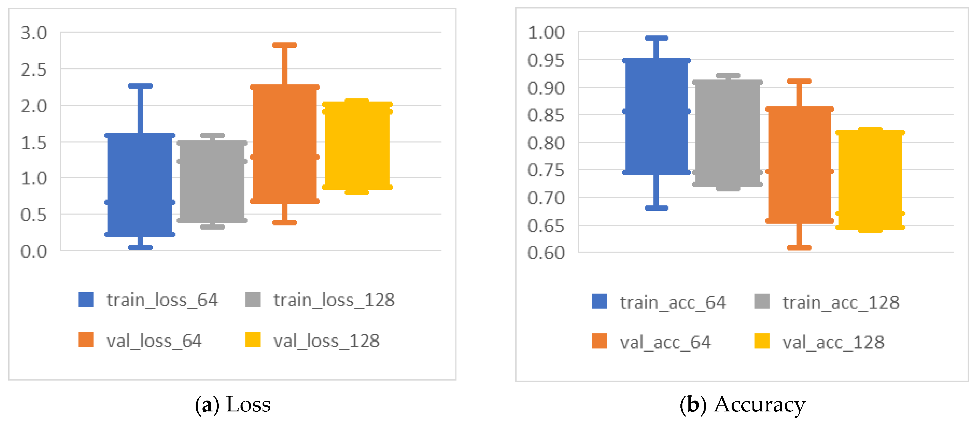
We trained the AlexNet model across 45 iteration, adjusting the batch size, learning rate, and number of epochs. The top three results for each dataset are presented in Table 3. The tested batch sizes were 64 and 128, and the best results are as follows:
  • J_OR—batch size 64 performed best, as expected due to the relatively small number of images in this dataset.
  • J_4x—both batch sizes showed satisfactory results.
  • J_16x—batch size 128 yielded the best results.
Figure 4 illustrates loss and accuracy variation (values shown on the Y-axis) during training and validation for J_4x considering batch sizes of 64 and 128. The learning rate varied from 0.01 to 0.0015.
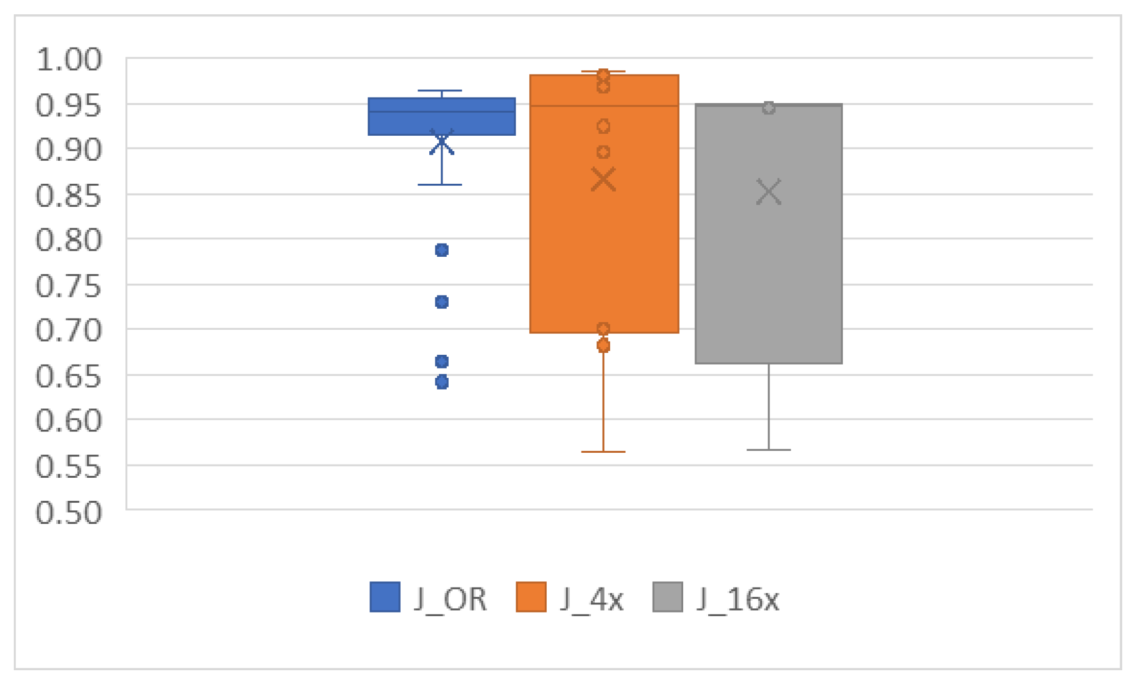
The best results were achieved with a learning rate of 0.0015 for all datasets. We evaluated the algorithm using 15, 50, 60 and 75 epochs. Table 3 shows that the smaller the dataset, the larger the number of epochs required for training, with the best results achieved with 50 or more epochs. Figure 5 shows the loss variation for five tests performed with the J_OR dataset using the parameters: learning rate = 0.0015, epochs = 75, and batch size = 64. Figure 5a illustrates the loss in training, which presents few variations and shows a descending curve with values closer to zero beginning in epoch 50. Figure 5b shows the loss in validation, which varies considerably until epoch 15 but tends to approach zero after epoch 50. In both cases, the loss values are presented on the Y-axis.
The training time was significantly reduced using a GPU. For the J_OR dataset, the training took 3 min with the GPU, compared to 60 min on the CPU. Similarly, the J_4x dataset required 6 min on the GPU, whereas it took 5 h when using the CPU. As for J_16x, it completed training in 16 min on the GPU, though it was not tested on the CPU due to the platform’s time limitations. The optimal hyperparameters for AlexNet were: Learning rate = 0.0015; Number of epochs ≥ 50 and ≤75; and Batch size = 64 for the J_OR dataset, and 128 for the other datasets.
For DenseNet-121, the model was also trained over 45 iterations, similarly to AlexNet. The top three results for each dataset are summarized in Table 4.
The batch size was fixed at 64 owing to hardware limitations, as processing with a batch size of 128 exceeded the available 25.45 GB of RAM.
The learning rates evaluated were 0.001, 0.0015 and 0.0001. We also varied the learning rate between executions, and no significant differences were observed in the results. The best results were achieved with a learning rate of 0.001 for datasets J_4x and J_16x.
Figure 6 presents the accuracy variation for DenseNet-121 across the datasets, with accuracy values shown on the Y-axis. The optimal hyperparameters were: Learning rate = 0.001; Number of epochs = 25; and Batch size = 64.
The conducted experiments and simulations show that AlexNet and DenseNet-121 both achieve high training and validation accuracy across different datasets, but several patterns emerged that help explain the models’ performance.
  • Batch size differences: For AlexNet, the smaller batch size (64) was optimal for J_OR, likely because of the limited number of images, which matches findings from other studies where small datasets perform better with smaller batch sizes. In contrast, J_16x benefited from a larger batch size (128), possibly due to the larger number of training instances generated from cropping, allowing for more stable gradient updates.
  • Epochs and dataset size: Larger datasets, such as J_4x and J_16x, achieved optimal results with fewer epochs compared to J_OR. Figure 5 provides insight into the loss progression, where training loss for J_OR decreased steadily after epoch 50, while validation loss fluctuated more but stabilized after epoch 50 as well. This indicates that smaller datasets require more epochs for the network to learn effectively, while larger datasets can converge more quickly. This aligns with standard DL practices, where smaller datasets often require more epochs to compensate for the lack of diversity in the training data.
  • Learning rate: Both models showed that a learning rate of 0.0015 (AlexNet) and 0.001 (DenseNet-121) consistently produced the best results. This suggests that the slightly lower learning rate helps prevent overshooting during optimization, which is particularly useful when training deeper models like DenseNet-121.
  • Model comparison: DenseNet-121 outperformed AlexNet in both training and validation accuracy across all datasets, particularly on J_4x and J_16x, with validation accuracies reaching as high as 98.5%. This is expected, given DenseNet-121’s more advanced architecture, which promotes efficient gradient flow through the network, leading to better generalization.
DenseNet-121 generally achieved higher validation accuracy than AlexNet across the three dataset variants (J_OR, J_4x, J_16x; see Table 3 and Table 4). We interpret this advantage as stemming from DenseNet’s dense feature propagation, which promotes feature reuse and improves gradient flow, enabling the network to capture the fine-grained textural and morphological cues characteristic of bacterial micrographs (e.g., contour sharpness, texture granularity, staining heterogeneity). AlexNet, while computationally lighter, offers less capacity to integrate multi-scale features, which likely limits its peak performance on these data.
Best configurations (synthesis). Across runs, AlexNet achieved its top results with batch size 64 on J_OR and 128 on J_4x/J_16x, with learning rate 0.0015 and ≥50 epochs. DenseNet-121 was constrained to batch size 64; the best learning rate was 0.001 on J_4x/J_16x, with 25 epochs for cropped sets and 50 epochs for J_OR. These settings correspond to the top entries summarized in Table 3 and Table 4.

4.2. Analysis of the Effects of Image Compression

In this section, the impact of image compression on the accuracy of CNNs is investigated. Two types of compression, lossless and lossy, are evaluated using the datasets P_OR, P_4x, and P_16x for lossless compression and the datasets J50_OR, J50_4x, and J50_16x (50% compression), J75_OR, J75_4x, and J75_16x (75% compression), and J95_OR, J95_4x, and J95_16x (95% compression) for lossy compression. The validation accuracy results are compared between the compression methods for both AlexNet and DenseNet-121 architectures.
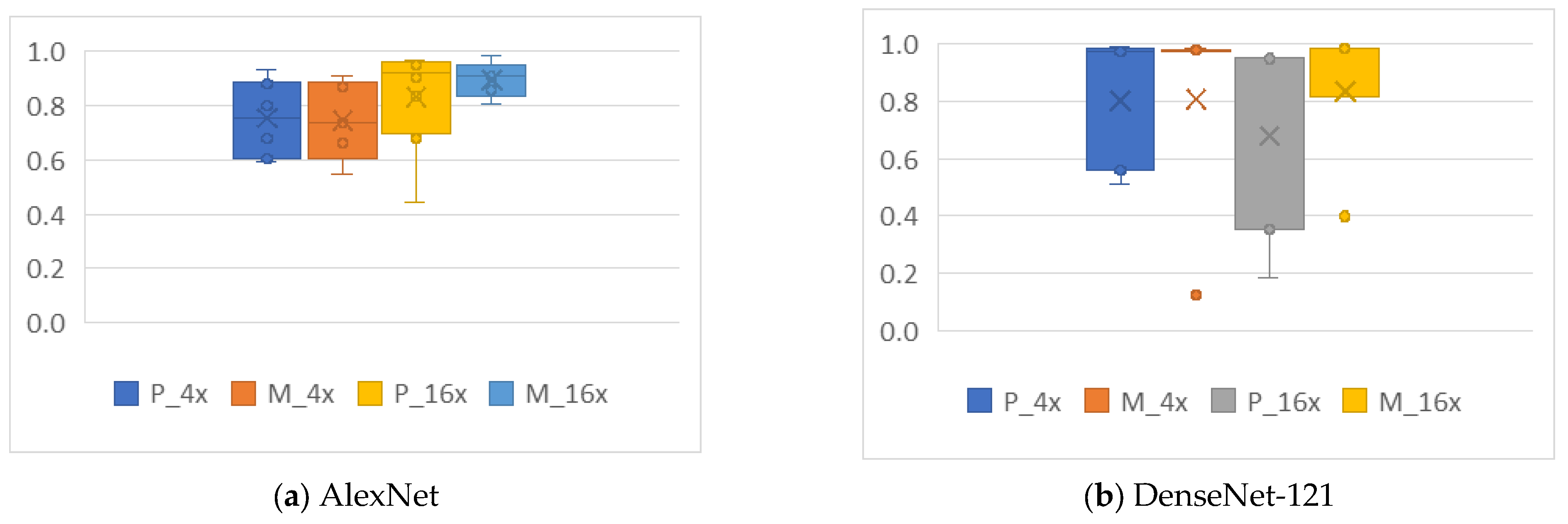
Ten training runs were executed using AlexNet and five using DenseNet-121, with the datasets P_OR, P_4x, and P_16x (lossless compression). These results were compared with those for the datasets J_OR, J_4x, and J_16x (95% lossy compression). An overview of this comparison, expressed through boxplots (which summarize statistical measures such as mean and variance), is shown in Figure 7a for AlexNet and Figure 7b for DenseNet-121. As indicated for the previous figure, accuracy values are shown on the Y-axis.
For AlexNet, the lossless compression datasets performed better, with the best results observed for P_16x and J_16x. For DenseNet-121, the maximum accuracies were similar between the compression types, but the lossless datasets showed higher variance.
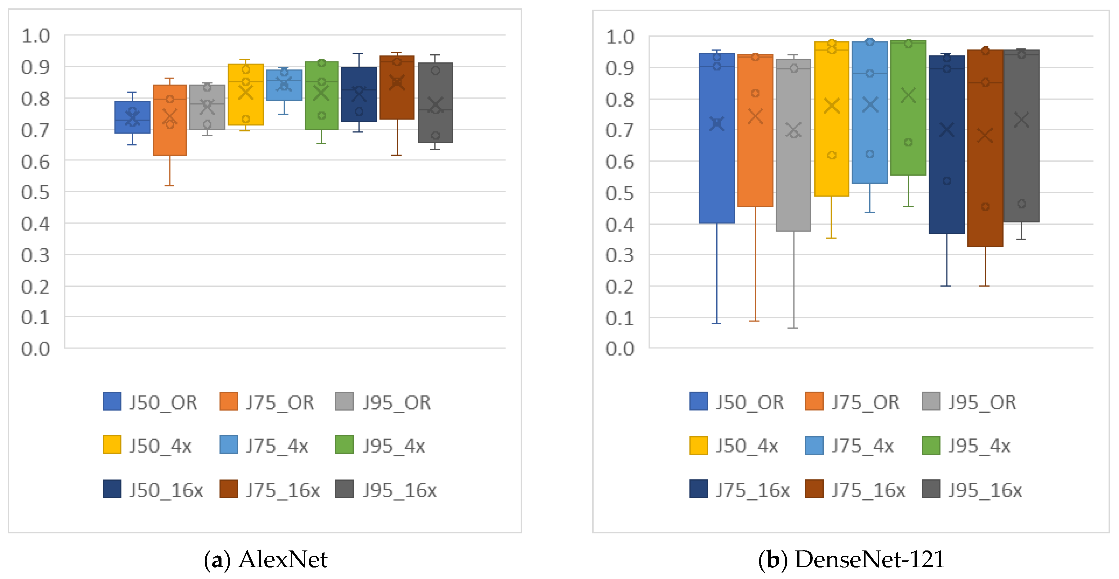
Next, to further investigate the effects of image quality on accuracy at different compression levels, both CNNs were trained five times using datasets converted to JPG (lossy compression): J50_OR, J50_4x, and J50_16x (50% compression), J75_OR, J75_4x, and J75_16x (75% compression), and J95_OR, J95_4x, and J95_16x (95% compression).
A comparison of the results is illustrated in Figure 8a for AlexNet and Figure 8b for DenseNet-121. Both CNNs achieved better results for datasets with 95% lossy compression. AlexNet performed best with the 16x datasets, while DenseNet-121 showed better performance with the 4x datasets. In general, DenseNet-121 performance remained relatively consistent across all compression levels, demonstrating strong generalization capacity.
Regarding the loss at different compression rates, the 75% and 95% compression rates show similar results for both CNNs. Moreover, DenseNet-121 presents equivalent results across all compression rates.
For AlexNet, the results show that lossless compression datasets generally produced better validation accuracies than lossy compression datasets. These findings suggest that preserving image quality through lossless compression benefits AlexNet, which lacks connections between layers, making it more susceptible to performance degradation when image quality is reduced through compression. For DenseNet-121, the results show that the maximum accuracies were similar across both lossless and lossy datasets. However, the variance in results was higher for the lossless datasets, indicating that DenseNet-121’s performance is more resilient to image compression compared to AlexNet. This may be due to the dense connections in DenseNet-121, which facilitate better information flow and mitigate the negative effects of compression.
The observed sensitivity to lower JPEG quality factors is consistent with the loss of high-frequency textures (e.g., granularity and edge definition) that are discriminative for species-level classification in microscopy images [56,57,58].
These insights contribute to a better understanding of how image compression influences CNN performance and can help guide future research in optimizing model training with compressed data [56,58,59].

4.3. Analysis of the Effects of Non-Uniform Scalings

In this section, we explore the effects of non-uniform scaling on CNNs performance. Since the original images have dimensions of 2048 × 1532 pixels, they are resized to meet the input size requirements of the CNNs. Specifically, AlexNet input images are resized to 227 × 227 pixels, while those for DenseNet-121 are resized to 224 × 224 pixels. Our original images have dimensions of 2048 × 1532 pixels. This resizing process involves non-uniform scaling, since the original images are rectangular, and the input layer requires square images.
To assess the impact of non-uniform scaling on CNN learning, we created the D_OR dataset, which consists of images resized to dimensions that maintain the aspect ratio for each CNN input layer. These are obtained by cropping the OR with the largest possible dimensions (1532 × 1532 pixels). For comparison with other experiments, additional datasets—D_4x (766 × 766 pixels) and D_16x (383 × 383 pixels)—were generated. These datasets contain the same number of images as in the 4x and 16x from other experiments. The scaling of these images to the required dimensions was invariant, allowing for comparison with the results obtained by the datasets that underwent non-uniform scaling (P_OR, P_4x, and P_16x). The accuracy results from the datasets that underwent uniform and non-uniform scaling are presented in Figure 9 and Figure 10.
From these results, it is evident that the number of images in the dataset influences the accuracy. The datasets with more images achieved better accuracy results, with DenseNet-121 consistently showing the best results across all datasets. Furthermore, the results for D_4x and D_16x were quite similar, which suggests that DenseNet-121 exhibits a better ability to generalize than AlexNet. Multi-scale crops expose complementary morphological context (cell size/shape and local texture), which benefits architectures that reuse features across layers (e.g., DenseNet-121).
As shown in Figure 10, datasets subjected to uniform scaling (D_OR, D_4x, and D_16x) consistently achieved higher validation accuracy for both CNNs, with less variance observed compared to datasets subjected to non-uniform scaling (P_OR, P_4x, and P_16x).
The results underscore the importance of scaling methods in CNN performance. Uniform scaling was found to provide a more consistent learning environment, allowing both AlexNet and DenseNet-121 to achieve higher accuracies, in line with prior observations on resolution choice and CNN accuracy [57]. The reduced variance in results for datasets subjected to uniform scaling further suggests that this preprocessing method ensures better learning consistency.
Moreover, the comparison between the two CNN architectures revealed that DenseNet-121 demonstrated superior performance and greater resilience to scaling-induced variations. This highlights DenseNet-121’s robust generalization ability, making it a suitable choice for tasks where variations in image dimensions or aspects are inevitable.
These findings provide important insights into how different scaling methods impact CNN training and suggest that uniform scaling can be an effective strategy for improving performance, especially when dealing with datasets with varying image dimensions.

4.4. Analysis of the Effects of Data Augmentation

This section presents the outcomes of experiments assessing the effects of data augmentation techniques on CNN accuracy, using both AlexNet and DenseNet-121 architectures. Augmentation methods—cropping, mirroring, rotation, and noise addition—were applied individually and in combination to the datasets.

4.4.1. Cropping

Cropping is a data augmentation technique frequently used in DL, particularly when high-resolution images are available, as in the DIBaS (2048 × 1532 pixels). In this context, cropping enables generating multiple images from a single source without sacrificing critical information for microorganism identification.
To evaluate this, two datasets were created: P_227 (37,206 images of 227 × 227 pixels for AlexNet) and P_224 (37,206 images of 224 × 224 pixels for DenseNet-121). These cropped images were generated by sequentially cropping from the original images, ensuring no overlapping areas to maximize unique content. This technique was feasible given the original image resolution, which permitted partitions that still preserved key microorganism details up to a limit, as excessive partitioning could remove essential features.
Further datasets were created by randomly selecting images from P_227 and P_224, mirroring the size of datasets P_OR, P_4x, and P_16x, named, respectively, as S_OR, S_4x, and S_16x. This setup standardized the dimensions and number of images, enabling the analysis of CNN accuracy as a function of image quantity without the influence of scaling. Notably, some cropped images where blank, containing only the background; however, these images were present in all datasets and influenced the classification accuracy in all experiments.
The results in Figure 11 reveal the effect of dataset size on learning. When the dataset is too small, as in S_OR, which contains 689 images, learning is impaired for both CNNs. However, for datasets with more than 2000 images, such as S_4x and S_16x, there is an increase in accuracy. Notably, DenseNet-121 showed higher accuracy variance than AlexNet, although its maximum accuracies surpassed those achieved by AlexNet.
An additional analysis compared validation accuracies above 0.7 for lossy (J), lossless (P), and cropped lossless (S) compression images, shown in Figure 12. For AlexNet, lossless compression images (P_OR, P_4x, and P_16x) exhibit the highest accuracy, followed by lossy compression (J_OR, J_4x, and J_16x), which does not occur for DenseNet-121. However, the cropped lossless compression images (S_OR, S_4x, and S_16x) present the worst accuracy results for both CNNs, suggesting that cropping negatively impacts the results. This result can be attributed to the fact that the cropped images (224 × 224 and 227 × 227 pixels) lacked sufficient representative information about the microorganisms for reliable identification. As shown in Figure 13, these cropped samples capture less structural, textural, and compositional detail, which hinders accurate classification.
The findings underscore that while cropping is a practical data augmentation method, it must be carefully applied in high-detail recognition tasks, such as microorganism identification. Preserving essential microorganism features in cropped images is crucial for increasing the training set. Failure to retain these fundamental features can substantially undermine CNN performance, highlighting the need for careful consideration when employing data augmentation techniques like cropping.
From this experiment, several additional conclusions can be drawn. The results confirm that the number of images in the dataset significantly impacts the learning performance of CNNs. Larger datasets generally lead to higher accuracy, as seen with datasets containing more than 2000 images. This highlights the necessity of a sufficiently large dataset to achieve optimal performance in training DL models. Additionally, the lower accuracy observed with cropped images suggests that the resolution and detail of the images are crucial for accurate microorganism identification.
Cropping can lead to a loss of important structural and textural information, which negatively affects the model’s ability to classify the images correctly. This implies that retaining high-resolution and detailed images is important for training effective models. Moreover, the experiment indicates that AlexNet and DenseNet-121 respond differently to data augmentation techniques like cropping. DenseNet-121 shows higher variance in accuracy compared to AlexNet, even though it achieves higher maximum accuracies. This suggests that DenseNet-121 may be more sensitive to changes in the input data and requires careful handling of data augmentation techniques to maintain consistent performance. Furthermore, the use of cropped images as a data augmentation technique involves trade-offs. While it increases the size of the training set, it may also introduce images that lack sufficient detail for accurate classification. Therefore, it is essential to balance the benefits of increasing the dataset size with the potential drawbacks of losing important image information. As alternatives, region-focused approaches (e.g., object detection or attention-based multiple-instance learning) could preserve broader context while emphasizing informative regions; we leave this for future work.

4.4.2. Mirroring

In this experiment, the impact of data augmentation through image mirroring on the performance of CNNs is evaluated. The original images of the P_OR dataset were mirrored in three different ways: horizontally (axis), vertically (x-axis), and both horizontally and vertically (x and y axes). Example images of the mirroring process are shown in Figure 14.
The mirrored images, along with the original images, were added to create the M_4x dataset, containing 2756 images. Then, each image was divided into four equal parts, generating the M_16x dataset with 11,024 images. The datasets created have approximately the same number of images as those of the other experiments. The CNN performance for these datasets is shown in Figure 15.
The results in Figure 15 show an accuracy increase and less variation for dataset M_16x compared to M_4x using AlexNet. The DenseNet-121 maximum accuracies are similar, with the highest variation occurring for the M_16x dataset. Again, this confirms that a large number of images helps AlexNet learning, but for DenseNet-121, this may not be necessary.
In Figure 16, the results obtained using the datasets without augmentation by mirroring (P_4x and P_16x) are compared with the results with mirroring (M_4x and M_16x). For AlexNet, it can be noted that there was no increase in accuracy, but M_16x showed less variation in the results. In contrast, for DenseNet-121, the mirroring technique not only reduced variation but also resulted in increased accuracy for M_16x.
This experiment also underscores the importance of dataset quality and size in training DL models. By increasing the number of training images through mirroring, the models, particularly DenseNet-121, achieve better performance. This reinforces the idea that having a larger and more diverse training set is beneficial for CNN training. Implementing mirroring as a data augmentation technique is straightforward and computationally inexpensive, making it an attractive option for enhancing datasets. This practical ease of use, combined with the observed benefits, supports the adoption of mirroring in various DL applications where increasing dataset size and diversity is desired.
In real-world applications where acquiring large, labeled datasets is often a challenge, data augmentation techniques like mirroring can be invaluable. They allow for the effective utilization of available data, improving model robustness and performance without the need for extensive additional data collection.
Mirroring as an augmentation strategy provides a way to address dataset limitations by artificially increasing the size and diversity of the data. The fact that DenseNet-121 performed better with the augmented data emphasizes the advantages of leveraging augmentation techniques like mirroring to increase the robustness and accuracy of deep learning models, especially for architectures like DenseNet-121, which benefit from the added diversity in the dataset.
Overall, this study suggests that mirroring is a valuable technique for improving CNN training. It offers an effective and simple solution to enhance dataset size and variability, making it particularly useful for applications where obtaining more data is challenging, especially for architectures like DenseNet-121.

4.4.3. Rotation

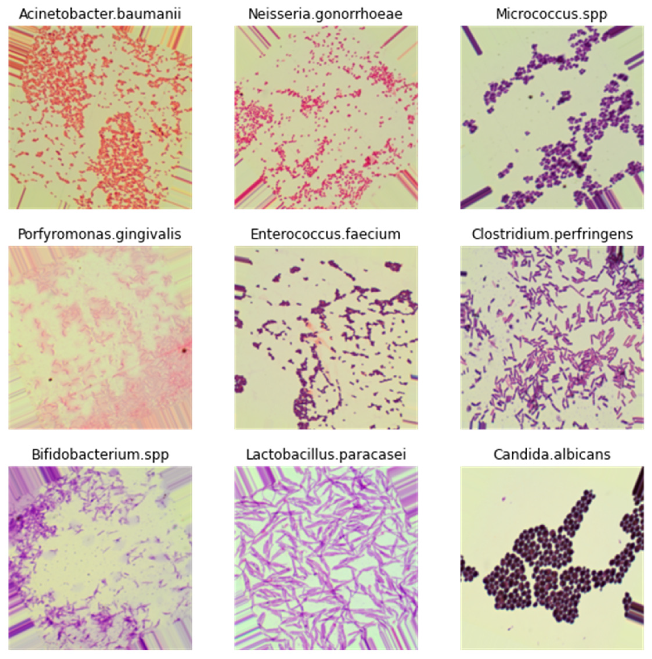
In this experiment, we evaluate the impact of image rotation as a data augmentation technique on the accuracy of CNNs. Two types of rotation were tested: fixed rotations (90°, 180° and 270°), for which datasets R_4x and R_16x were created, and random rotations (from 0° to 90° counterclockwise), for which datasets A_4x and A_16x were created. It is important to note that for random rotation, the “black” spaces left by the operation were filled with a background reproducing the image characteristics, making the rotated images more like the original ones. Examples of rotated images are shown in Figure 17.
The rotated and the original images were added to the *_4x dataset, resulting in 2756 images. The *_4x dataset images were cut into four equal parts, generating the *_16x dataset with 11,024 images. With this, the datasets created have approximately the same number of images as those of the other experiments. The performance results are presented in Figure 18.
For AlexNet, the 90°, 180°, and 270° rotations negatively interfered with learning, as there was no significant gain in accuracy and large variation in performance results. This could be attributed to variations in input image dimensions. Specifically, 90° and 270° rotations create dimensions that are inverted relative to the original images, causing more distortions during the scaling process. For DenseNet, the same negative impact is observed for dataset R_4x but not for R_16x, showing better generalization than AlexNet and confirming that a larger dataset helps in learning.
The graph in Figure 19 presents the validation accuracy results obtained for original (P_4x and P_16x), rotated at 90°, 180°, and 270° (R_4x and R_16x), and randomly rotated (A_4x and A_16x) images.
Random rotations exhibit a positive influence on the validation accuracy results for AlexNet, as there was an increase in the maximum accuracy and less variance. This becomes more evident when the accuracy results obtained with data augmentation by rotation are compared with the original images (P_4x and P_16x) results. It can be observed in the graph of Figure 19 that there is almost no difference between the results for original and rotated 90°, 180°, and 270° images; however, the results obtained for randomly rotated images show higher accuracies and lower variance. For the DenseNet-121, on the other hand, there is no noticeable difference in the accuracy results, which, again, shows that it has a greater generalization capacity.
The experiment on image rotation as a data augmentation technique reveals contrasting effects for AlexNet and DenseNet-121. For AlexNet, fixed rotations of 90°, 180°, and 270° resulted in minimal gains and high variation in accuracy. This suggests that these rotations distort the image dimensions, particularly with 90° and 270° rotations, where the image’s aspect ratio is inverted. These distortions likely complicate the learning process by introducing inconsistencies between the original and rotated images. DenseNet-121 showed similar results for the R_4x dataset but exhibited better generalization with the R_16x dataset, where a larger number of images helped mitigate the impact of fixed rotations. DenseNet-121’s superior ability to handle variations in input data highlights its robustness over AlexNet.
Random rotation (from 0° to 90°) had a more positive effect on both CNNs. For AlexNet, it resulted in higher accuracy and reduced variance, suggesting that random rotation helps the model generalize by introducing diverse transformations. This approach allows AlexNet to better handle different orientations of objects, improving its robustness. For DenseNet-121, random rotation did not significantly affect performance, reinforcing its capacity for generalization even without augmentation. DenseNet-121’s resilience to rotational changes underscores its effectiveness in handling varied input data without the need for additional transformations.
The results indicate that random rotation is a more effective augmentation technique than fixed-angle rotations. While fixed rotations degraded performance, particularly for AlexNet, due to image distortions, random rotation introduced beneficial variation without such drawbacks. This improved both the accuracy and generalization of AlexNet, whereas DenseNet-121, due to its higher robustness, showed minimal sensitivity to the added transformations. These findings suggest that random rotation can be a valuable strategy for enhancing the performance of less complex CNNs like AlexNet, but may have limited impact on more resilient architectures such as DenseNet-121.

4.4.4. Noise

In this experiment, the impact of adding noise to images as a data augmentation technique was evaluated. Three types of noise were applied to the images of the P_OR dataset: Gaussian, salt and pepper, and Poisson noise. Datasets N_4x and N_16x were created for these experiments, and the results are shown in Figure 20.
The results shown in Figure 20 indicate that for the AlexNet, there was a considerable increase in accuracy for the _4x datasets, and for the _16x, there was an increase in variance. As for the DenseNet-121, there was no significant gain in accuracy, but there was a reduction in variance. These findings suggest that noise addition has varying impacts on the performance of the two models, especially when the dataset size increases.
The addition of noise as a data augmentation technique demonstrated several interesting effects on both AlexNet and DenseNet-121, which can be interpreted in the context of dataset size and model architecture. The considerable increase in accuracy for AlexNet with the N_4x dataset suggests that adding noise can enhance the model’s ability to generalize from limited data, which is particularly beneficial in scenarios where obtaining large, clean datasets is challenging. However, the increased variance observed in AlexNet’s performance on the N_16x dataset indicates that while noise can be helpful, it can also introduce instability when the dataset size is significantly increased. This underscores the need for careful tuning of noise levels to balance accuracy gains and performance stability.
In contrast, the reduced variance in DenseNet-121’s performance suggests that this model is inherently more robust to the introduction of noise, making it advantageous for applications where data quality cannot always be controlled. Unlike traditional machine learning algorithms, which often suffer from degraded performance with noisy data, CNNs can leverage noise to improve generalization. This capability is a significant advantage, highlighting CNNs’ resilience and adaptability to real-world data imperfections.
The contrasting responses of AlexNet and DenseNet-121 to noise addition emphasize the varying sensitivity of different architectures to noise. This variability should be considered when designing augmentation strategies tailored to specific models. Noise addition increases the diversity of the training dataset without requiring additional data collection efforts, which is particularly useful in fields where data acquisition is expensive or time-consuming.
The findings suggest that in applications where noise is an unavoidable aspect of data, such as medical imaging or remote sensing, CNNs can be trained to handle such noise effectively, ensuring reliable performance despite imperfect data.

4.5. Summary of Results, Limitations, Practical Implications, and Future Directions

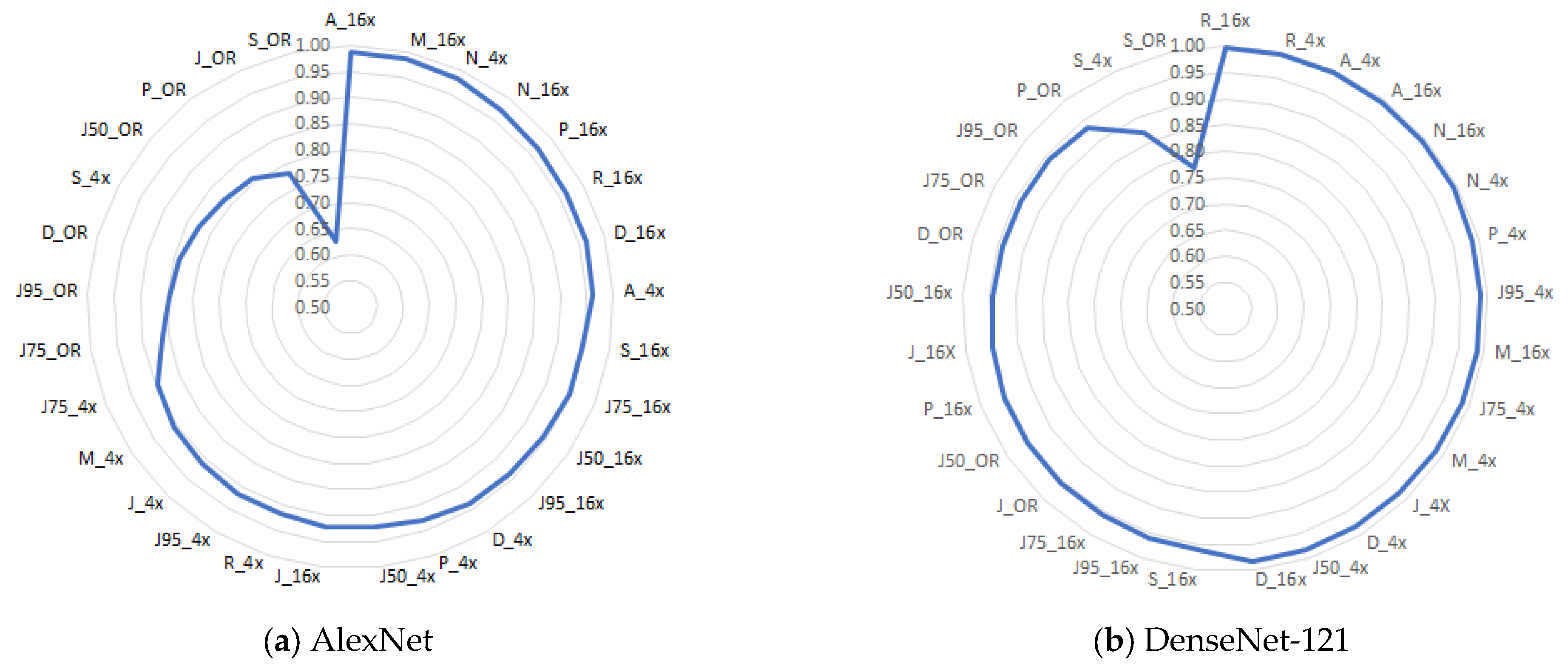
The comparison of the maximum accuracy results across all experiments, as shown in Figure 21 and Table 5, reveals several key trends. Datasets created through data augmentation with the highest number of images (_4x and _16x) consistently achieve higher accuracy results than smaller datasets. Specifically, the _16x datasets, which contain over 10,000 images, demonstrate superior performance, particularly with AlexNet, which is a simpler CNN compared to DenseNet-121.
DenseNet-121 consistently presents excellent results, achieving over 90% accuracy for nearly all datasets, which highlights its superior generalization capability even with smaller datasets.
Among the datasets with the highest number of images (_16x), the accuracies illustrated in Figure 22 confirm that extensive data augmentation significantly enhances learning outcomes for both CNNs. However, cropped images (S_16x) yield the worst accuracy results for both models, indicating the necessity of maintaining minimum dimensions to preserve sufficient patterns for microorganism identification.
Additionally, comparing compressed and cropped images, it is evident that lossless compression generally provides better accuracy than lossy compression or cropping, particularly for AlexNet, consistent with prior analyses of compression and DL performance [56,58]. This suggests that preserving image quality through lossless compression is crucial for maintaining high classification accuracy. In contrast, DenseNet-121’s comparable performance with lossy compression demonstrates its robustness to some reduction in data quality.
The findings provide valuable insights for optimizing model training with augmented data. They emphasize the importance of maintaining high image quality and ensuring a sufficiently large dataset size. Researchers should carefully assess the impact of various data augmentation techniques on their specific models and datasets.
Comparison between the results for both CNNs shows that AlexNet is efficient for smaller datasets and limited hardware environments, offering stable performance under basic preprocessing. However, it has limited capacity to generalize with complex augmentations and tends to achieve lower maximum accuracy due to its simpler architecture. DenseNet-121, in contrast, benefits from dense feature propagation, leading to superior generalization and robustness under extensive data augmentation. It consistently outperforms AlexNet in complex scenarios but demands higher computational resources and is more sensitive to hyperparameter tuning. It is also important to highlight that both AlexNet and DenseNet-121 were trained from scratch on the DIBaS dataset, without using pretrained ImageNet weights. This strengthens the novelty of our approach, as the high performance observed can be attributed to the preprocessing strategies and hyperparameter optimization rather than transfer learning. In summary, while AlexNet is a resource-friendly option for simpler tasks, DenseNet-121 delivers higher accuracy and better resilience to transformations, making it preferable for complex datasets—provided adequate computational capacity is available.
The best results observed were 98.61% accuracy for AlexNet and 99.82% for DenseNet-121. These results are superior to those reported in the literature, where the best result obtained with the AlexNet for cell classification was 96.63% [20], and for classification of microorganisms, using the DIBaS dataset, was 97.24% [54]. This demonstrates that your data augmentation techniques and the use of DenseNet-121 have significantly improved performance compared to the previously reported results.
Morphology-preserving augmentations (e.g., rotations, flips, mild brightness/contrast changes) enhance robustness to routine laboratory variability, whereas more aggressive transforms risk distorting diagnostically relevant cues.
The knowledge generated in this study, including the meticulous parameterization of CNNs, attention to detail in the preparation of input images, and strategic application of data augmentation, collectively contributed to the substantial improvement in CNN performance.
A notable limitation is this study’s focus on the DIBaS dataset, which may reduce generalizability to other domains within biological imaging, including variability across laboratories in staining protocols, imaging hardware, and sample preparation, as well as differences in magnification levels and imaging modalities [59]; external validation on multi-center datasets will be required to assess robustness under such acquisition differences. Additionally, while data augmentations such as noise and random rotations were beneficial here, their impact may vary with other datasets or tasks, particularly if augmentations introduce inconsistencies or distortions. To mitigate performance drops when using lower-quality or degraded images, we found that preserving image quality, as in the case of lossless compression over cropping, remains crucial.
Another limitation is that we relied on an 80/20 train–validation split rather than k-fold cross-validation. While repeated runs with different random seeds confirmed the stability of our results, future work should incorporate k-fold validation to further strengthen robustness. In addition, our evaluation primarily reports accuracy; future work will include per-class precision, recall, F1 score, and confusion matrices to provide a more granular assessment. We did not retain per-sample predictions across runs, which precluded paired significance tests (e.g., McNemar’s) and resampling-based uncertainty estimates in this revision; future work will store predictions to enable formal statistical comparisons between preprocessing conditions and architectures.
Furthermore, DenseNet-121 delivers higher accuracy at greater computational cost and usually higher activation memory during training; although it has fewer parameters than AlexNet, its dense connectivity increases runtime cost. This trade-off should guide model choice for resource-constrained deployments.
While this study focused on CNN architectures, emerging alternatives such as Vision Transformers (ViTs) are gaining traction in medical imaging. A recent systematic review by [60] highlighted the advantages of ViTs in capturing long-range dependencies and their potential to complement CNNs across radiology, pathology, and microscopy tasks. Future work should therefore explore the integration of ViTs or hybrid CNN-ViT approaches for microorganism classification, which may further enhance robustness and generalization in biomedical applications.
This study’s findings have several practical implications for healthcare, particularly in diagnostic settings where large, labeled datasets are often limited. Augmentation techniques can increase model robustness and accuracy without the need for costly data acquisition. DenseNet-121’s robustness makes it suitable for applications where computational resources allow, while AlexNet could serve in more constrained environments for simpler tasks. Practically, DenseNet-121 suits high-stakes or well-resourced workflows, while AlexNet is viable for constrained deployments; in both cases, image quality and morphology-preserving augmentation are key. Additionally, the lack of model interpretability, inherent to CNNs, presents a barrier to clinical implementation. Future work should prioritize interpretability to ensure clinical trust and acceptance. Expanding CNN applications to combine microorganism classification with data from other medical imaging modalities may also offer comprehensive diagnostic support, further enhancing CNN utility in healthcare.
Our results suggest that CNNs hold considerable promise for accurate microorganism classification, especially with sufficient data and quality augmentation. However, adapting these models for broader clinical applications will require balancing interpretability, computational feasibility, and rigorous validation across varied datasets. Future efforts should also explore other data augmentation methods and enhance the interpretability of CNN models, as indicated in [61].

5. Conclusions

This study systematically evaluated how commonly used image preprocessing practices—such as data compression, non-uniform scaling, and data augmentation—affect the performance of CNNs in microorganism classification. Using AlexNet and DenseNet-121, we conducted experiments and simulations on a standardized bacterial image dataset, identifying how each preprocessing strategy can either degrade or enhance CNN performance depending on specific conditions.
For automated microorganism classification in Laboratory 4.0 settings, DenseNet-121’s higher accuracy and robustness suggest it as the preferred backbone when computational resources permit—particularly where misclassification costs are high. AlexNet remains attractive for resource-constrained deployments (e.g., embedded microscopes, edge devices) where inference speed and memory footprint are critical. In all cases, careful control of image quality and morphology-preserving augmentation is essential for reliable performance.
Through our experiments, we demonstrated how to carefully prepare training sets to optimize CNN performance. Then, using the insights produced in this research, we achieved results that surpassed those reported in previous studies considering the same dataset, demonstrating the effectiveness of our approach.
Our findings provide actionable insights into the challenges and trade-offs involved in training CNNs under real-world constraints. They support the development of robust and efficient models not only for Laboratory 4.0 environments but also for broader applications in remote diagnostics, quality control, and environmental monitoring. Moreover, this study offers practical guidance for researchers working with limited biological datasets, highlighting how preprocessing strategies can be tailored to maximize model performance.
Future research could build upon our work by evaluating additional CNN architectures and exploring advanced data augmentation strategies, such as using generative AI to create synthetic training images. Furthermore, enhancing the interpretability of CNN models remains crucial for understanding their predictive mechanisms and facilitating their integration with other imaging modalities in more comprehensive diagnostic frameworks.

Author Contributions

The authors confirm contribution to the paper as follows: D.T.B.: conceptualization, methodology, writing—original draft, software, formal analysis and validation, writing—review and editing, funding acquisition, and supervision. M.A.S.B.: formal analysis, validation, and writing—review and editing. H.D.: formal analysis and validation. A.M.D.: formal analysis and validation. P.A.B.: formal analysis, and validation. S.A.d.A.: conceptualization, methodology, writing—original draft, formal analysis, validation, writing—review and editing, funding acquisition, and project administration. All authors have read and agreed to the published version of the manuscript.

Funding

This work was supported by the National Council for Scientific and Technological Development (CNPq) through research grants (processes 421769/2023-8 and 313484/2025-2) awarded to S. A. Araújo. We declare that the funding institution had no involvement in the study design; collection, analysis and interpretation of data; writing of the report; and in the decision to submit the article for publication.

Institutional Review Board Statement

Bias in Training Data: We meticulously curated our training dataset to ensure balanced representation of microorganism species. Table 1 demonstrates our efforts, with approximately equal numbers of images used for each species, mitigating biases towards specific organisms. Algorithmic Bias: While our dataset encompasses a diverse range of microorganism species, its selection was constrained by available literature. We acknowledge potential biases arising from this limitation and have undertaken measures to mitigate them through careful dataset curation and model evaluation. Data Privacy and Security: Our study’s focus on microorganism image classification alleviates direct data privacy concerns. Nonetheless, we adhere to ethical guidelines governing the responsible handling and storage of research data to safeguard participant privacy and confidentiality. Potential Harm from Incorrect Predictions: It is essential to view the CNN models developed herein as decision support tools, not definitive diagnostic instruments. Users should exercise caution when interpreting model predictions, treating them as guidance rather than absolute truth. The inclusion of probability scores alongside predictions aids users in assessing the confidence level of the model’s classifications. Transparency and Accountability: We prioritize transparency across our research process, from dataset collection and model development to evaluation and result interpretation. Encouraging open discussion and scrutiny of our methodologies and findings fosters accountability and trustworthiness in our research endeavors. By addressing these ethical considerations, we endeavor to advocate for responsible utilization of CNNs in microorganism classification and contribute to the promotion of ethical AI practices within scientific research.

Data Availability Statement

The data used in this study were obtained from the publicly available Digital Images of Bacteria Species (DIBaS) dataset, available at: https://doctoral.matinf.uj.edu.pl/database/dibas/ (accessed on 13 February 2022; no longer available; Now it is mirrored in https://github.com/gallardorafael/DIBaS-Dataset?utm_source=chatgpt.com (accessed on 5 August 2025)). All images used were preprocessed as described in Section 3.2 and Section 3.3. The code for conducting experiments is available in a GitHub repository: https://github.com/dtbouk-droid/microlab-cnn (accessed on 5 August 2025).

Acknowledgments

The authors acknowledge the Conselho Nacional de Desenvolvimento Científico e Tecnológico (CNPq) for awarding the Research Grants (Processes 421769/2023-8 and 313484/2025-2) to S. A. Araújo, as well as the UNINOVE for their continued institutional support.

Conflicts of Interest

The authors declare no conflict of interest.

Appendix A

Table A1. Datasets used in the experiments.
Sub-
Dataset
DescriptionResolution (in Pixels)Number of Images
J_OROR converted to JPG (lossy compression)1532 × 2048689
J_4xJ_OR cropped in 4 parts766 × 10242756
J_16xJ_OR cropped in 16 parts383 × 51211,024
J_227J_OR cropped in 227 × 227 pixels images (AlexNet)227 × 22737,206
J_224J_OR cropped in 224 × 224 pixels images (DenseNet-121)224 × 22437,206
J50_OROR converted to JPG (50% lossy compression)1532 × 2048689
J50_4xJ50_OR cropped in 4 parts766 × 10242756
J50_16xJ50_OR cropped in 16 parts383 × 51211,024
J75_OROR converted to JPG (75% lossy compression)1532 × 2048689
J75_4xJ75_OR cropped in 4 parts766 × 10242756
J75_16xJ75_OR cropped in 16 parts383 × 51211,024
J95_OROR converted to JPG (95% lossy compression)1532 × 2048689
J95_4xJ95_OR cropped in 4 parts766 × 10242756
J95_16xJ95_OR cropped in 16 parts383 × 51211,024
P_OROR converted to PNG (lossless compression)1532 × 2048689
P_4xP_OR cropped in 4 parts766 × 10242756
P_16xP_OR cropped in 16 parts383 × 51211,024
P_227P_OR cropped images with 227 × 227 pixels (AlexNet)227 × 22737,206
P_224P_OR cropped images with 224 × 224 pixels (DenseNet-121)224 × 22437,206
S_ORRandom images from P_227 or P_2241532 × 2048689
S_4xRandom images from P_227 or P_224766 × 10242756
S_16xRandom images from P_227 or P_224383 × 51211,024
D_ORP_OR cropped (using the largest possible dimension)1532 × 1532689
D_4xD_OR cropped in 4 parts766 × 7662756
D_16xD_OR cropped in 16 parts383 × 38311,024
M_4xP_OR mirrowed in x, in y, and in x and y1532 × 15322756
M_16xM_4x cropped in 4 parts766 × 76611,024
R_4xP_OR rotated by 90, 180 and 270 degrees1532 × 20482756
R_16xR_4x cropped in 4 parts766 × 102411,024
A_4xP_OR rotated randomly from 0 to 90 degrees1532 × 20482756
A_16xA_4x cropped in 4 parts766 × 102411,024
N_4xP_OR noise added1532 × 20482756
N_16xN_4x cropped in 4 parts766 × 102411,024

References

  1. Tortora, G.J.; Funke, B.R.; Case, C.L. Microbiologia, 10th ed.; Artmed Editora: Porto Alegre, Brazil, 2012; ISBN 978-85-363-2584-0. [Google Scholar]
  2. World Health Organization. WHO Coronavirus Disease (COVID-19) Dashboard with Vaccination Data|WHO Coronavirus (COVID-19) Dashboard with Vaccination Data; World Health Organization: Geneva, Switzerland, 2022; pp. 1–5. [Google Scholar]
  3. Alom, M.Z.; Taha, T.M.; Yakopcic, C.; Westberg, S.; Sidike, P.; Nasrin, M.S.; Hasan, M.; Van Essen, B.C.; Awwal, A.A.S.; Asari, V.K. A state-of-the-art survey on deep learning theory and architectures. Electronics 2019, 8, 292. [Google Scholar] [CrossRef]
  4. Jo, Y.J.; Park, S.; Jung, J.H.; Yoon, J.; Joo, H.; Kim, M.-H.; Kang, S.-J.; Choi, M.C.; Lee, S.Y.; Park, Y. Holographic deep learning for rapid optical screening of anthrax spores. Sci. Adv. 2017, 3, e1700606. [Google Scholar] [CrossRef] [PubMed]
  5. Savardi, M.; Ferrari, A.; Signoroni, A. Automatic hemolysis identification on aligned dual-lighting images of cultured blood agar plates. Comput. Methods Programs Biomed. 2018, 156, 13–24. [Google Scholar] [CrossRef] [PubMed]
  6. Kulwa, F.; Li, C.; Zhang, J.; Shirahama, K.; Kosov, S.; Zhao, X.; Jiang, T.; Grzegorzek, M. A new pairwise deep learning feature for environmental microorganism image analysis. Environ. Sci. Pollut. Res. 2022, 29, 51909–51926. [Google Scholar] [CrossRef]
  7. Lewy, D.; Mańdziuk, J. An overview of mixing augmentation methods and augmentation strategies. Artif. Intell. Rev. 2022, 56, 2111–2169. [Google Scholar] [CrossRef]
  8. Alzubaidi, L.; Zhang, J.; Humaidi, A.J.; Al-Dujaili, A.; Duan, Y.; Al-Shamma, O.; Santamaría, J.; Fadhel, M.A.; Al-Amidie, M.; Farhan, L. Review of Deep Learning: Concepts, CNN Architectures, Challenges, Applications, Future Directions; Springer International Publishing: Cham, Switzerland, 2021; Volume 8. [Google Scholar] [CrossRef]
  9. Taye, M.M. Theoretical Understanding of Convolutional Neural Network: Concepts, Architectures, Applications, Future Directions. Computation 2023, 11, 52. [Google Scholar] [CrossRef]
  10. Angermueller, C.; Pärnamaa, T.; Parts, L.; Stegle, O. Deep learning for computational biology. Mol. Syst. Biol. 2016, 12, 878. [Google Scholar] [CrossRef]
  11. Cao, C.; Liu, F.; Tan, H.; Song, D.; Shu, W.; Li, W.; Zhou, Y.; Bo, X.; Xie, Z. Deep Learning and Its Applications in Biomedicine. Genom. Proteom. Bioinform. 2018, 16, 17–32. [Google Scholar] [CrossRef]
  12. Mahmud, M.; Kaiser, M.S.; Hussain, A.; Vassanelli, S. Applications of Deep Learning and Reinforcement Learning to Biological Data. IEEE Trans. Neural Netw. Learn. Syst. 2018, 29, 2063–2079. [Google Scholar] [CrossRef]
  13. Moen, E.; Bannon, D.; Kudo, T.; Graf, W.; Covert, M.; Van Valen, D. Deep learning for cellular image analysis. Nat. Methods 2019, 16, 1233–1246. [Google Scholar] [CrossRef]
  14. Karagoz, M.A.; Akay, B.; Basturk, A.; Karaboga, D.; Nalbantoglu, O.U. An unsupervised transfer learning model based on convolutional auto encoder for non-alcoholic steatohepatitis activity scoring and fibrosis staging of liver histopathological images. Neural Comput. Appl. 2023, 35, 10605–10619. [Google Scholar] [CrossRef]
  15. Poostchi, M.; Silamut, K.; Maude, R.J.; Jaeger, S.; Thoma, G. Image analysis and machine learning for detecting malaria. Transl. Res. 2018, 194, 36–55. [Google Scholar] [CrossRef]
  16. Mienye, I.D.; Swart, T.G.; Obaido, G.; Jordan, M.; Ilono, P. Deep Convolutional Neural Networks in Medical Image Analysis: A Review. Information 2025, 16, 195. [Google Scholar] [CrossRef]
  17. Wu, Y.; Gadsden, S.A. Machine learning algorithms in microbial classification: A comparative analysis. Front. Artif. Intell. 2023, 6, 1200994. [Google Scholar] [CrossRef]
  18. Schäfer, R.; Nicke, T.; Höfener, H.; Lange, A.; Merhof, D.; Feuerhake, F.; Schulz, V.; Lotz, J.; Kiessling, F. Overcoming data scarcity in biomedical imaging with a foundational multi-task model. Nat. Comput. Sci. 2024, 4, 495–509. [Google Scholar] [CrossRef]
  19. Hegde, R.B.; Prasad, K.; Hebbar, H.; Singh, B.M.K. Comparison of traditional image processing and deep learning approaches for classification of white blood cells in peripheral blood smear images. Biocybern. Biomed. Eng. 2019, 39, 382–392. [Google Scholar] [CrossRef]
  20. Sharma, M.; Bhave, A.; Janghel, R.R. White blood cell classification using convolutional neural network. Adv. Intell. Syst. Comput. 2019, 900, 135–143. [Google Scholar] [CrossRef]
  21. Hay, E.A.; Parthasarathy, R. Performance of convolutional neural networks for identification of bacteria in 3D microscopy datasets. PLoS Comput. Biol. 2018, 14, 1–17. [Google Scholar] [CrossRef]
  22. Xu, Y.; Noy, A.; Lin, M.; Qian, Q.; Li, H.; Jin, R. WeMix: How to Better Utilize Data Augmentation. arXiv 2020, arXiv:2010.01267. [Google Scholar] [CrossRef]
  23. Benbarrad, T.; Kably, S.; Arioua, M.; Alaoui, N. Compression-Based Data Augmentation for CNN Generalization. In International Conference on Cybersecurity, Cybercrimes, and Smart Emerging Technologies; Springer International Publishing: Cham, Switzerland, 2021; pp. 235–244. [Google Scholar] [CrossRef]
  24. Krizhevsky, A.; Sutskever, I.; Hinton, G.E. ImageNet classification with deep convolutional neural networks. Commun. ACM 2017, 60, 84–90. [Google Scholar] [CrossRef]
  25. Huang, G.; Liu, Z.; Van Der Maaten, L.; Weinberger, K.Q. Densely Connected Convolutional Networks. In Proceedings of the IEEE Conference on Computer Vision and Pattern Recognition (CVPR), Honolulu, HI, USA, 21–26 July 2017; pp. 4700–4708. [Google Scholar] [CrossRef]
  26. Benbarrad, T.; Eloutouate, L.; Arioua, M.; Elouaai, F.; Laanaoui, M.D. Impact of image compression on the performance of steel surface defect classification with a CNN. J. Sens. Actuator Networks 2021, 10, 73. [Google Scholar] [CrossRef]
  27. Alfio, V.S.; Costantino, D.; Pepe, M. Influence of image tiff format and jpeg compression level in the accuracy of the 3d model and quality of the orthophoto in uav photogrammetry. J. Imaging 2020, 6, 30. [Google Scholar] [CrossRef]
  28. Shorten, C.; Khoshgoftaar, T.M. A survey on Image Data Augmentation for Deep Learning. J. Big Data 2019, 6, 60. [Google Scholar] [CrossRef]
  29. Sornam, M.; Muthusubash, K.; Vanitha, V. A Survey on Image Classification and Activity Recognition using Deep Convolutional Neural Network Architecture. In Proceedings of the 9th International Conference on Advanced Computing, Ho Chi Minh City, Vietnam, 27–29 November 2018; IEEE: Piscataway, NJ, USA, 2018; pp. 121–126. [Google Scholar] [CrossRef]
  30. Van Valen, D.A.; Kudo, T.; Lane, K.M.; Macklin, D.N.; Quach, N.T.; DeFelice, M.M.; Maayan, I.; Tanouchi, Y.; Ashley, E.A.; Covert, M.W. Deep Learning Automates the Quantitative Analysis of Individual Cells in Live-Cell Imaging Experiments. PLoS Comput. Biol. 2016, 12, e1005177. [Google Scholar] [CrossRef] [PubMed]
  31. Ferrari, A.; Lombardi, S.; Signoroni, A. Bacterial colony counting with Convolutional Neural Networks in Digital Microbiology Imaging. Pattern Recognit. 2017, 61, 629–640. [Google Scholar] [CrossRef]
  32. López, Y.P.; Costa Filho, C.F.F.; Aguilera, L.M.R.; Costa, M.G.F. Automatic classification of light field smear microscopy patches using Convolutional Neural Networks for identifying Mycobacterium Tuberculosis. In Proceedings of the 2017 CHILEAN Conference on Electrical, Electronics Engineering, Information and Communication Technologies (CHILECON), Pucon, Chile, 18–20 October 2017. [Google Scholar] [CrossRef]
  33. Sadanandan, S.K.; Ranefall, P.; Le Guyader, S.; Wählby, C. Automated Training of Deep Convolutional Neural Networks for Cell Segmentation. Sci. Rep. 2017, 7, 7860. [Google Scholar] [CrossRef] [PubMed]
  34. Xu, X.; Qin, J.; Guo, J. Gram staining of intestinal flora classification based on convolutional neural network. In Proceedings of the 2017 IEEE 19th International Conference on e-Health Networking, Applications and Services (Healthcom), Dalian, China, 12–15 October 2017. [Google Scholar] [CrossRef]
  35. Kim, G.; Jo, Y.; Cho, H.; Choi, G.; Kim, B.S.; Min, H.S.; Park, Y. Automated Identification of Bacteria Using Threedimensional Holographic Imaging and Convolutional Neural Network. In Proceedings of the 2018 IEEE Photonics Conference (IPC), Reston, VA, USA, 30 September 2018–4 October 2018. [Google Scholar]
  36. Wahid, M.F.; Ahmed, T.; Habib, M.A. Classification of microscopic images of bacteria using deep convolutional neural network. In Proceedings of the 2018 10th International Conference on Electrical and Computer Engineering (ICECE), Dhaka, Bangladesh, 20–22 December 2018; pp. 217–220. [Google Scholar] [CrossRef]
  37. Tamiev, D.; Furman, P.E.; Reuel, N.F. Automated classification of bacterial cell subpopulations with convolutional neural networks. PLoS ONE 2020, 15, e0241200. [Google Scholar] [CrossRef]
  38. Cubuk, E.D.; Zoph, B.; Shlens, J.; Le, Q.V. RandAugment: Practical Automated Data Augmentation with a Reduced Search Space. arXiv 2019, arXiv:1909.13719. [Google Scholar] [CrossRef]
  39. Faryna, K.; Van Der Laak, J.; Litjens, G. Tailoring automated data augmentation to H&E-stained histopathology. In Proceedings of the Machine Learning Research, Hangzhou, China, 17–19 September 2021; Available online: https://proceedings.mlr.press/v143/faryna21a.html (accessed on 5 August 2025).
  40. LeCun, Y.; Bottou, L.; Bengio, Y.; Haffner, P. Gradient-based learning applied to document recognition. Proc. IEEE 1998, 86, 2278–2323. [Google Scholar] [CrossRef]
  41. Szegedy, C.; Vanhoucke, V.; Ioffe, S.; Shlens, J. Rethinking the Inception Architecture for Computer Vision. In Proceedings of the IEEE Conference on Computer Vision and Pattern Recognition (CVPR), Las Vegas, NV, USA, 27–30 June 2016; pp. 2818–2826. [Google Scholar] [CrossRef]
  42. Huang, L.; Wu, T. Novel neural network application for bacterial colony classification. Theor. Biol. Med. Model. 2018, 15, 22. [Google Scholar] [CrossRef]
  43. Yu, W.; Chang, J.; Yang, C.; Zhang, L.; Shen, H.; Xia, Y.; Sha, J. Automatic classification of leukocytes using deep neural network. In Proceedings of the 2017 IEEE 12th International Conference on ASIC (ASICON), Guiyang, China, 25–28 October 2017; pp. 1041–1044. [Google Scholar] [CrossRef]
  44. Dubey, A.; Singh, S.K.; Jiang, X. Leveraging CNN and Transfer Learning for Classification of Histopathology Images. In International Conference on Machine Learning, Image Processing, Network Security and Data Sciences; Springer International Publishing: Cham, Switzerland, 2022; Volume 1763, pp. 3–13. [Google Scholar] [CrossRef]
  45. Panicker, R.O.; Kalmady, K.S.; Rajan, J.; Sabu, M.K. Automatic detection of tuberculosis bacilli from microscopic sputum smear images using deep learning methods. Biocybern. Biomed. Eng. 2018, 38, 691–699. [Google Scholar] [CrossRef]
  46. Bellenberg, S.; Buetti-Dinh, A.; Galli, V.; Ilie, O.; Herold, M.; Christel, S.; Boretska, M.; Pivkin, I.V.; Wilmes, P.; Sand, W.; et al. Automated microscopic analysis of metal sulfide colonization by acidophilic microorganisms. Appl. Environ. Microbiol. 2018, 84, e01835-18. [Google Scholar] [CrossRef]
  47. Costa, M.G.F.; Filho, C.F.F.C.; Kimura, A.; Levy, P.C.; Xavier, C.M.; Fujimoto, L.B. A sputum smear microscopy image database for automatic bacilli detection in conventional microscopy. In Proceedings of the 2014 36th Annual International Conference of the IEEE Engineering in Medicine and Biology Society, Chicago, IL, USA, 26–30 August 2014; pp. 841–2844. [Google Scholar] [CrossRef]
  48. Kuok, C.P.; Horng, M.H.; Liao, Y.M.; Chow, N.H.; Sun, Y.N. An effective and accurate identification system of Mycobacterium tuberculosis using convolution neural networks. Microsc. Res. Tech. 2019, 82, 709–719. [Google Scholar] [CrossRef]
  49. Smith, K.P.; Kang, A.D.; Kirby, J.E. Automated interpretation of blood culture gram stains by use of a deep convolutional neural network. J. Clin. Microbiol. 2018, 56, e01521-17. [Google Scholar] [CrossRef] [PubMed]
  50. Zieliński, B.; Plichta, A.; Misztal, K.; Spurek, P.; Brzychczy-Włoch, M.; Ochońska, D. Deep learning approach to bacterial colony classification. PLoS ONE 2017, 12, e0184554. [Google Scholar] [CrossRef] [PubMed]
  51. Xue, Y.; Ray, N.; Hugh, J.; Bigras, G. Cell counting by regression using convolutional neural network. In Lecture Notes in Computer Science; Including Subseries Lecture Notes in Artificial Intelligence and Lecture Notes in Bioinformatics; Springer International Publishing: Cham, Switzerland, 2016; Volume 9913, pp. 274–290. [Google Scholar] [CrossRef]
  52. Qin, F.; Gao, N.; Peng, Y.; Wu, Z.; Shen, S.; Grudtsin, A. Fine-grained leukocyte classification with deep residual learning for microscopic images. Comput. Methods Programs Biomed. 2018, 162, 243–252. [Google Scholar] [CrossRef]
  53. Shahin, A.I.; Guo, Y.; Amin, K.M.; Sharawi, A.A. White blood cells identification system based on convolutional deep neural learning networks. Comput. Methods Programs Biomed. 2019, 168, 69–80. [Google Scholar] [CrossRef] [PubMed]
  54. Zieliski, B.; Sroka-Oleksiak, A.; Rymarczyk, D.; Piekarczyk, A.; Brzychczy-Woch, M. Deep learning approach to describe and classify fungi microscopic images. PLoS ONE 2020, 15, e0234806. [Google Scholar] [CrossRef]
  55. Sajedi, H.; Mohammadipanah, F.; Pashaei, A. Image-processing based taxonomy analysis of bacterial macromorphology using machine-learning models. Multimed Tools Appl. 2020, 79, 32711–32730. [Google Scholar] [CrossRef]
  56. Dodge, S.; Karam, L. Understanding how image quality affects deep neural networks. In Proceedings of the 2016 Eighth International Conference on Quality of Multimedia Experience (QoMEX), Lisbon, Portugal, 6–8 June 2016. [Google Scholar] [CrossRef]
  57. Kannojia, S.P.; Jaiswal, G. Effects of Varying Resolution on Performance of CNN based Image Classification An Experimental Study. Int. J. Comput. Sci. Eng. 2018, 6, 451–456. [Google Scholar] [CrossRef]
  58. Chen, Y.; Janowczyk, A.; Madabhushi, A. Quantitative Assessment of the Effects of Compression on Deep Learning in Digital Pathology Image Analysis. JCO Clin. Cancer Inform. 2020, 4, 221–233. [Google Scholar] [CrossRef]
  59. Yip, M.Y.T.; Lim, G.; Lim, Z.W.; Nguyen, Q.D.; Chong, C.C.Y.; Yu, M.; Bellemo, V.; Xie, Y.; Lee, X.Q.; Hamzah, H.; et al. Technical and imaging factors influencing performance of deep learning systems for diabetic retinopathy. npj Digit. Med. 2020, 3, 31–34. [Google Scholar] [CrossRef] [PubMed]
  60. Takahashi, S.; Sakaguchi, Y.; Kouno, N.; Takasawa, K.; Ishizu, K.; Akagi, Y.; Aoyama, R.; Teraya, N.; Bolatkan, A.; Shinkai, N.; et al. Comparison of Vision Transformers and Convolutional Neural Networks in Medical Image Analysis: A Systematic Review. J. Med. Syst. 2024, 48, 84. [Google Scholar] [CrossRef] [PubMed]
  61. Aknda, M.R.; Farid FAl Uddin, J.; Mansor, S.; Kibria, M.G. SCCM: An Interpretable Enhanced Transfer Learning Model for Improved Skin Cancer Classification. BioMedInformatics 2025, 5, 43. [Google Scholar] [CrossRef]
Figure 2. Comparison of DIBas with other datasets source from the literature. Source: [55].
Biomedinformatics 05 00061 g002
Figure 3. Examples of cropping of an original (OR) image with 1532 × 2048 pixels.
Biomedinformatics 05 00061 g003
Figure 4. Loss and accuracy variation during training and validation for J_4x, considering batch sizes of 64 and 128.
Biomedinformatics 05 00061 g004
Figure 5. Training and validation loss for the J_OR dataset.
Biomedinformatics 05 00061 g005
Figure 6. DenseNet-121 accuracy variation for datasets J_OR, J_4x, and J_16x, considering batch size of 64.
Biomedinformatics 05 00061 g006
Figure 7. Validation accuracy for datasets P_OR, P_4x, and P_16x (lossless compression) and J_OR, J_4x, and J_16x (lossy compression).
Biomedinformatics 05 00061 g007
Figure 8. Validation accuracy obtained for the JPG (lossy compression) datasets: J50_OR, J50_4x, and J50_16x (50% compression), J75_OR, J75_4x, and 75_16x (75% compression), and J95_OR, J95_4x, and J95_16x (95% compression).
Biomedinformatics 05 00061 g008
Figure 9. Validation accuracy for images that underwent uniform scaling.
Biomedinformatics 05 00061 g009
Figure 10. Validation accuracies for images obtained through non-uniform scaling (P_OR, P_4x, and P_16x) and uniform scaling (D_OR, D_4x, and D_16x).
Biomedinformatics 05 00061 g010
Figure 11. Validation accuracies for datasets S_OR, S_4x and S_16x.
Biomedinformatics 05 00061 g011
Figure 12. Accuracies above 0.7 for lossy (J), lossless (P), and cropped lossless compression (S) images.
Biomedinformatics 05 00061 g012
Figure 13. Examples of original images and respective cropped images, (a) Original images and (b) Cropped images.
Biomedinformatics 05 00061 g013
Figure 14. Examples of image mirroring. (a) Original image, (b) Horizontal mirroring, (c) Vertical mirroring, and (d) Vertical and horizontal mirroring.
Biomedinformatics 05 00061 g014
Figure 15. Accuracies for the datasets augmented by mirroring.
Biomedinformatics 05 00061 g015
Figure 16. Accuracy comparison for datasets without (P_4x and P_16x) and with data augmentation by mirroring (M_4x and M_16x).
Biomedinformatics 05 00061 g016
Figure 17. Images randomly rotated from 0° to 90° counterclockwise.
Biomedinformatics 05 00061 g017
Figure 18. Validation accuracies for data augmentation by image rotation.
Biomedinformatics 05 00061 g018
Figure 19. Comparison of accuracy results for (a) AlexNet and (b) DenseNet-121.
Biomedinformatics 05 00061 g019
Figure 20. Validation accuracies for the addition of noise.
Biomedinformatics 05 00061 g020
Figure 21. Top accuracies obtained in the experiments for (a) AlexNet and (b) DenseNet-121.
Biomedinformatics 05 00061 g021
Figure 22. Comparison between accuracies of (a) AlexNet (b) DenseNet-121 for _16x.
Biomedinformatics 05 00061 g022
Table 1. DIBaS dataset list of bacteria and respective image quantities.
BacteriaNumber of ImagesBacteriaNumber of Images
Acinetobacter baumanii20Lactobacillus plantarum20
Actinomyces israeli23Lactobacillus reuteri20
Bacteroides fragilis23Lactobacillus rhamnosus20
Bifidobacterium spp.23Lactobacillus salivarius20
Candida albicans20Listeria monocytogenes22
Clostridium perfringens23Micrococcus spp21
Enterococcus faecalis20Neisseria gonorrhoeae23
Enterococcus faecium20Porfyromonas gingivalis23
Escherichia coli20Propionibacterium acnes23
Fusobacterium23Proteus20
Lactobacillus casei20Pseudomonas aeruginosa20
Lactobacillus crispatus20Staphylococcus aureus20
Lactobacillus delbrueckii20Staphylococcus epidermidis20
Lactobacillus gasseri20Staphylococcus saprophiticus20
Lactobacillus jehnsenii20Streptococcus agalactiae20
Lactobacillus johnsonii20Veionella22
Lactobacillus paracasei20------
Table 2. Hardware resources used in the Google Colab Pro platform.
ResourceGPU with Standard RAMGPU with High RAM
GPUA100-SXM4-40 GBTesla P100-PCIE-16 GB
RAM12.68 GB25.45 GB
Hard drive166.77 GB166.77 GB
CPU2 Intel® Xeon® 2.20 GHz4 Intel® Xeon® 2.20 GHz
Table 3. Top three AlexNet training and validation accuracy results for each dataset.
DatasetEpochsLearning Ra.Batch SizeAccuracy
TrainingValidation
J_16x500.00151280.99010.9533
J_16x500.00151280.97320.9369
J_16x500.00151280.97760.9351
J_4x750.0015640.98910.9111
J_4x750.00151280.92020.8221
J_4x750.0015640.90520.8094
J_OR750.0015640.94750.7810
J_OR750.001640.98370.7737
J_OR750.0015640.94750.7445
Table 4. Top three DenseNet-121 training and validation accuracy results for each dataset.
DatasetEpochsLearning RateBatch SizeAccuracy
TrainingValidation
J_OR500.0015640.99090.9635
J_OR500.001640.99460.9562
J_OR500.0001640.99090.9562
J_4x250.001640.99350.9855
J_4x250.001640.99170.9823
J_4x250.001640.99050.9809
J_16x250.001640.98210.9492
J_16x250.001640.98120.9474
J_16x250.001640.97810.9456
Table 5. Top accuracies obtained in the experiments for each CNN (in descending order).
AlexNetDenseNet-121AlexNetDenseNet-121
Datasetval_accDatasetval_accDatasetval_accDatasetval_acc
A_16x0.9861R_16x0.9982J_16x0.9211S_16x0.9605
M_16x0.9855R_4x0.9964R_4x0.9165J95_16x0.9596
N_4x0.9819A_4x0.9948J95_4x0.9165J75_16x0.9564
N_16x0.9732A_16x0.9946J_4x0.9111J_OR0.9562
P_16x0.9660N_16x0.9936M_4x0.9074J50_OR0.9562
R_16x0.9651N_4x0.9909J75_4x0.8966P_16x0.9551
D_16x0.9646P_4x0.9882J75_OR0.8613J_16X0.9492
A_4x0.9619J95_4x0.9868J95_OR0.8467J50_16x0.9437
S_16x0.9477M_16x0.9859D_OR0.8394D_OR0.9416
J75_16x0.9469J75_4x0.9850S_4x0.8271J75_OR0.9416
J50_16x0.9428M_4x0.9837J50_OR0.8175J95_OR0.9416
J95_16x0.9374J_4X0.9823P_OR0.8102P_OR0.9343
D_4x0.9365D_4x0.9819J_OR0.7810S_4x0.8711
P_4x0.9310J50_4x0.9819S_OR0.6277S_OR0.7737
J50_4x0.9238D_16x0.9814
Disclaimer/Publisher’s Note: The statements, opinions and data contained in all publications are solely those of the individual author(s) and contributor(s) and not of MDPI and/or the editor(s). MDPI and/or the editor(s) disclaim responsibility for any injury to people or property resulting from any ideas, methods, instructions or products referred to in the content.