
Voice as a Health Indicator: The Use of Sound Analysis and AI for Monitoring Respiratory Function


Abstract
1. Introduction
2. Materials and Methods
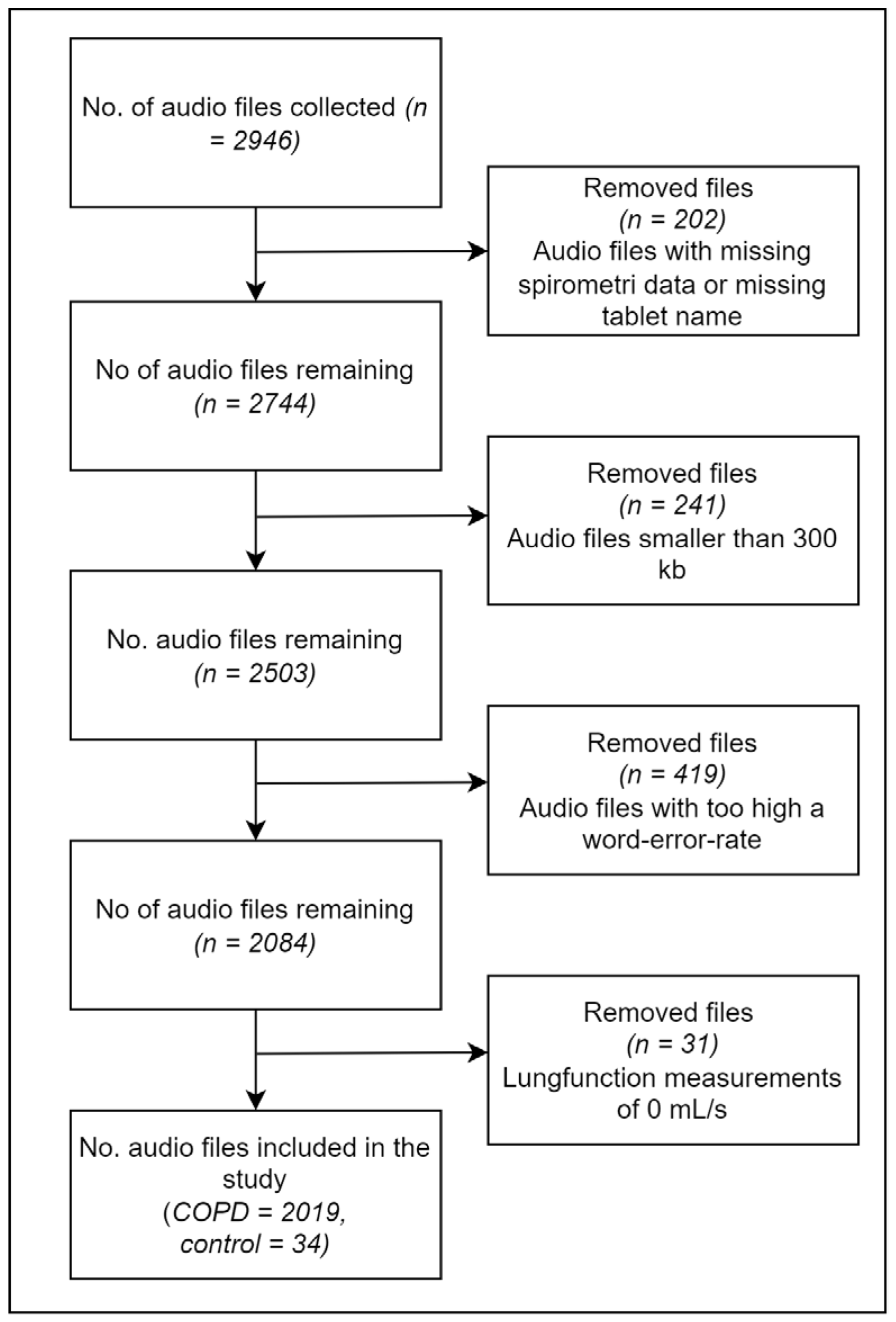
2.1. Data Processing
2.2. Feature Engineering
2.3. Feature Selection
2.4. Modeling
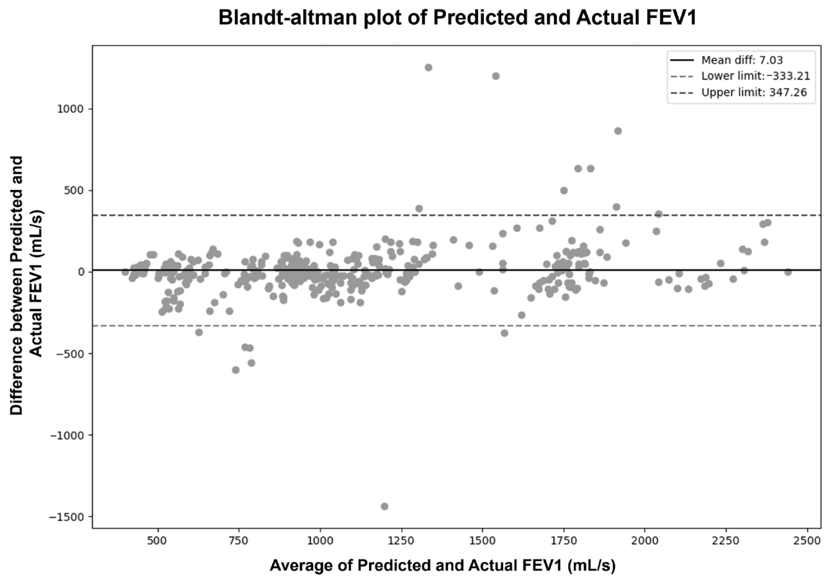
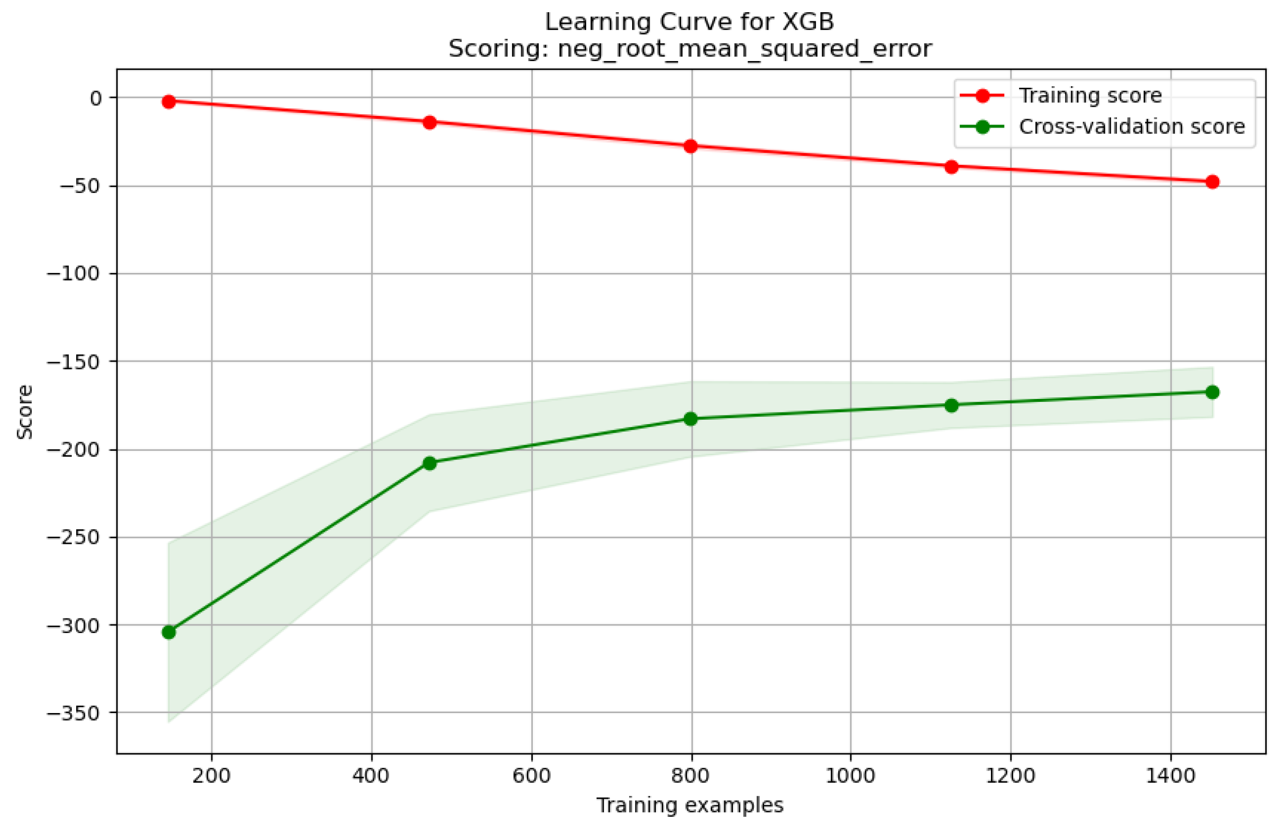
3. Results
4. Discussion
4.1. Model Performance
4.2. Feature Importance
4.3. Practical Considerations for At-Home Deployment
4.4. Limitations
5. Conclusions
Author Contributions
Funding
Institutional Review Board Statement
Informed Consent Statement
Data Availability Statement
Acknowledgments
Conflicts of Interest
Abbreviations
| Activation (MLP) | The function determining the output of a neuron given an input (e.g., ‘ReLU’, ‘tanh’). |
| Algorithm (KNN) | The method used to find the nearest neighbors (e.g., ‘ball_tree’, ‘kd_tree’, ‘brute’). |
| Alpha Regularization Parameter | Controls the penalty strength applied to model complexity to prevent overfitting (used for L1, L2, or both depending on the model). |
| Colsample_bytree (XGBoost) | The fraction of features (columns) considered when building each tree. |
| COPD | Chronic obstructive pulmonary disease |
| FEV1 | Forced expiratory volume in one second |
| Gamma (XGBoost) | Minimum loss reduction required to perform a further partition (split) on a leaf node of the tree; acts as a regularization parameter. |
| Hidden_layer_sizes (MLP) | Defines the architecture of the MLP, specifying the number of neurons in each hidden layer. |
| IQR | Interquartile range |
| KNN | K-nearest neighbors |
| L1_ratio (ElasticNet) | Specifies the mixing proportion between L1 (lasso) and L2 (ridge) penalties in ElasticNet regularization (0 = L2, 1 = L1). |
| Learning_rate | Controls the step size at each iteration while moving toward a minimum of the loss function; influences the convergence speed and stability (XGBoost, MLP). |
| LoA | Limit of agreement |
| MAE | Mean absolute error |
| MAPE | Mean absolute percentage error |
| Max_depth | The maximum depth allowed for individual decision trees in an ensemble, controlling model complexity. |
| Max_iter (MLP) | The maximum number of training iterations (epochs) allowed for the MLP solver to converge. |
| MFCC | Mel-frequency cepstral coefficient |
| Min_child_weight (XGBoost) | The minimum sum of instance weights needed in a child node; acts as a regularization parameter. |
| Min_samples_leaf | The minimum number of data samples required to be present in a leaf node of a decision tree. |
| Min_samples_split | The minimum number of data samples required within a node to allow it to be split further in a decision tree. |
| MLP | Multi-layer perceptron |
| MSE | Mean squared error |
| N_estimators | The number of decision trees included in the ensemble model (random forest, XGBoost). |
| N_neighbors (KNN) | The number of nearest neighbors considered to produce a prediction. |
| PCA | Principal component analysis |
| RF | Random forest |
| RFE | Recursive feature elimination |
| RMSE | Root mean squared error |
| Solver (MLP) | The algorithm used to optimize the weights of the MLP during training (e.g., ‘Adam’). |
| Subsample (XGBoost) | The fraction of the training data samples used to fit each individual tree. |
| Weights (KNN) | Specifies how the influence of neighbors is weighted in the predictions (e.g., ‘uniform’—all equal, ‘distance’—closer neighbors have a greater influence). |
| WER | Word error rate |
| XGB | XGBoost |
Appendix A
Appendix A.1. Sommerdrøm—Under et Blomstrende æbletræ Kumbel: Gruk—19
Appendix A.2. Den Første Gang Jeg Så Dig af Kim Larsen and Kjukken
Appendix A.3. Jeg Plukker Fløjlsgræs af Sigfred Pedersen and Knud Vad-Thomsen
Appendix A.4. Jeg Vil La’ Lyset Brænde af Ray Dee Ohh
Appendix B
Appendix C

| Feature | Explanation |
|---|---|
| Energy | The total magnitude of the signal, representing the amount of sound energy. |
| Entropy of Energy | The variation in energy throughout the signal, indicating dynamic changes. |
| Spectral Centroid | The balance point of the spectrum, indicating the brightness of a sound. |
| Spectral Spread | A measure of the spread of the spectrum, indicating the timbral texture. |
| Spectral Entropy | The randomness in the spectral amplitude distribution, a measure of signal complexity. |
| Spectral Flux | The rate of change in the spectral power, indicating the texture or timbral change. |
| Spectral Rolloff | The frequency below which a specified percentage of the total spectral energy lies. |
| Mel Frequency Cepstral Coefficient | Features that capture key aspects of the spectral envelope (shape of the power spectrum) of a sound, using the Mel frequency scale, which approximates human auditory perception. |
| Chroma Vector | A representation of the energy content within each pitch class, related to the harmonic and melodic content. |
| Chroma Deviation | The variation from a standard chroma vector, indicating deviations in harmonic content. |
| Zero Crossing Rate | The rate at which the signal changes sign, related to the frequency content of the signal. |
| Linear Predictive Coding | Coefficients derived from a model that predicts future signal samples based on past samples, often used to represent the vocal tract filter. |
| Word Error Rate | The rate of errors in speech transcription, indicating the accuracy of voice recognition. |
| Speech Pauses | The presence or duration of pauses in speech, potentially indicating respiratory issues or speech flow. |
| Heart Rate | The number of heart beats per minute, indicating cardiovascular health. |
| Body Temperature | The measured temperature of the body, an indicator of metabolic and overall health. |
| Oxygen Saturation | The percentage of oxygen carried by red blood cells to the body, indicating the respiratory efficiency. |
Appendix D
| Feature | Mean | Median | Standard Deviation | Max | IQR | Range | Non-Aggregated |
|---|---|---|---|---|---|---|---|
| Zero Crossing Rate | X | X | |||||
| Energy | |||||||
| Entropy of Energy | X | X | |||||
| Spectral Centroid | X | X | |||||
| Spectral Spread | X | ||||||
| Spectral Entropy | X | ||||||
| Spectral Rolloff | X | X | |||||
| MFCC | X | X | X | X | X | X | |
| Chroma Vector | X | X | X | X | X | X | |
| Chroma Deviation | |||||||
| Linear Predictive Coding | X | ||||||
| Pulse | X | ||||||
| Temperature | X | ||||||
| Hhmætning | X | ||||||
| World Error Rate | X | ||||||
| Speech Pauses | |||||||
| Relative Energi Difference | X | ||||||
| Delta Zero Crossing Rate | X | X | |||||
| Delta Energy | |||||||
| Delta Entropy of Energy | X | ||||||
| Delta Spectral Centroid | X | X | |||||
| Delta Spectral Spread | |||||||
| Delta Spectral Entropy | X | X | |||||
| Delta Spectral Rolloff | X | X | |||||
| Delta MFCC | X | X | X | ||||
| Delta Chroma Vector | X | X | X | ||||
| Delta Chroma Deviation | X | X | X |
References
- Bensoussan, Y.; Elemento, O.; Rameau, A. Voice as an AI Biomarker of Health—Introducing Audiomics. JAMA Otolaryngol. Head Neck Surg. 2024, 150, 283–284. [Google Scholar] [CrossRef] [PubMed]
- World Health Organization. Global Surveillance, Prevention and Control of Chronic Respiratory Diseases: A Comprehensive Approach; World Health Organization: Geneva, Switzerland, 2007.
- Kerkhof, M.; Voorham, J.; Dorinsky, P.; Cabrera, C.; Darken, P.; Kocks, J.W.H.; Sadatsafavi, M.; Sin, D.D.; Carter, V.; Tran, T.N.; et al. Association between COPD exacerbations and lung function decline during maintenance therapy. Thorax 2020, 75, 744–753. [Google Scholar] [CrossRef] [PubMed]
- Kakavas, S.; Kotsiou, O.S.; Perlikos, F.; Gourgoulianis, K.I.; Steiropoulos, P. Pulmonary function testing in COPD: Looking beyond the curtain of FEV1. NPJ Prim. Care Respir. Med. 2021, 31, 23. [Google Scholar] [CrossRef]
- Liu, X.L.; Tan, J.Y.; Wang, T.; Zhang, Q.; Zhang, M.; Yao, L.Q.; Chen, J.X. Effectiveness of home-based pulmonary rehabilitation for patients with chronic obstructive pulmonary disease: A meta-analysis of randomized controlled trials. Rehabil. Nurs. 2014, 39, 36–59. [Google Scholar] [CrossRef]
- Johnson, B.; Theobald, J.; Darcy, K.; Mottershaw, M.; Brassington, K.; Thickett, D.R. Improving spirometry testing by understanding patient preferences. ERJ Open Res. 2021, 7, 00766–02020. [Google Scholar] [CrossRef]
- Parsons, K.; Thomas, P.; Bevan-Smith, E.; Doran, O.; Sama, S. Patient perceived facilitators to greater self-management using home spirometry. Eur. Respir. J. 2022, 60, 2325. [Google Scholar] [CrossRef]
- Anand, R.; Topriceanu, C.C.; Keir, G.; Williamson, J.P.; Gao, J. Unsupervised home spirometry versus supervised clinic spirometry for respiratory disease: A systematic methodology review and meta-analysis. Eur. Respir. Rev. 2023, 32, 220135. [Google Scholar] [CrossRef] [PubMed]
- Sang, B.; Wen, H.; Junek, G.; Neveu, W.; Di Francesco, L.; Ayazi, F. An accelerometer-based wearable patch for robust respiratory rate and wheeze detection using deep learning. Biosensors 2024, 14, 118. [Google Scholar] [CrossRef]
- Minakata, Y.; Azuma, Y.; Sasaki, S.; Murakami, Y. Objective measurement of physical activity and sedentary behavior in patients with chronic obstructive pulmonary disease: Points to keep in mind during evaluations. J. Clin. Med. 2023, 12, 3254. [Google Scholar] [CrossRef]
- Wang, W.; Wan, Y.; Li, C.; Chen, Z.; Zhang, W.; Zhao, L.; Zhao, J.; Mu Li, G. Millimetre-wave radar-based spirometry for the preliminary diagnosis of chronic obstructive pulmonary disease. IET Radar Sonar Navig. 2023, 17, 1874–1885. [Google Scholar] [CrossRef]
- Islam, S.M.M. Radar-based remote physiological sensing: Progress, challenges, and opportunities. Front. Physiol. 2022, 13, 955208. [Google Scholar] [CrossRef] [PubMed]
- Alam, M.Z.; Patel, A.; Bui, F.M.; Fazel-Rezai, R.; Sazonov, E.; Bobhate, P.; Jaiswal, N.; Batsis, J.A.; Ramachandran, S.K.; McSharry, P.; et al. Predicting pulmonary function from the analysis of voice: A machine learning approach. Front. Digit. Health 2022, 4, 750226. [Google Scholar] [CrossRef] [PubMed]
- Nathan, V.; Paul, S.; Prioleau, T.; Niu, L.; Mortazavi, B.J.; Camargo, C.A.; Guttag, J.; Dy, J.; Jaimovich, D.; Colantonio, L.D.; et al. Assessment of chronic pulmonary disease patients using biomarkers from natural speech recorded by mobile devices. In Proceedings of the IEEE 16th International Conference on Wearable and Implantable Body Sensor Networks (BSN), Chicago, IL, USA, 19–22 May 2019. [Google Scholar] [CrossRef]
- Claxton, S.; Williams, G.; Roggen, D.; Rotheram, S.; Lam, C.; Howard, S.; Khawaja, S.; Price, D.B.; Crooks, M.G. Identifying acute exacerbations of chronic obstructive pulmonary disease using patient-reported symptoms and cough feature analysis. NPJ Digit. Med. 2021, 4, 107. [Google Scholar] [CrossRef] [PubMed]
- Xu, W.; Zhou, Y.; Zhao, M.; Wang, L.; Zhang, X.; Chen, Q.; Xie, Q.; Gao, B.; Li, B.; Shi, Y. A forced cough sound based pulmonary function assessment method by using machine learning. Front. Public Health 2022, 10, 1015876. [Google Scholar] [CrossRef] [PubMed]
- Radford, A.; Kim, J.W.; Xu, T.; Brockman, G.; McLeavey, C.; Sutskever, I. Robust speech recognition via large-scale weak supervision. In Proceedings of the International Conference on Machine Learning (ICML), Honolulu, HI, USA, 23–29 July 2023; PMLR 202. pp. 28491–28518. [Google Scholar]
- Mozilla. Common Voice Corpus v16.1. Available online: https://commonvoice.mozilla.org/da/datasets (accessed on 4 April 2024).
- Wiechern, B.; Liberty, K.A.; Pattemore, P.; Lin, E. Effects of asthma on breathing during reading aloud. Speech Lang. Hear. 2018, 21, 30–40. [Google Scholar] [CrossRef]
- Craney, T.A.; Surles, J.G. Model-Dependent Variance Inflation Factor Cutoff Values. Qual. Eng. 2002, 14, 391–403. [Google Scholar] [CrossRef]
- Kursa, M.B.; Rudnicki, W.R. Feature Selection with the Boruta Package. J. Stat. Softw. 2010, 36, 1–13. [Google Scholar] [CrossRef]
- Santamato, V.; Tricase, C.; Faccilongo, N.; Iacoviello, M.; Pange, J.; Marengo, A. Machine learning for evaluating hospital mobility: An Italian case study. Appl. Sci. 2024, 14, 6016. [Google Scholar] [CrossRef]
- Polisena, J.; Tran, K.; Cimon, K.; Hutton, B.; McGill, S.; Palmer, K.; Scott, R.E. Home telehealth for chronic obstructive pulmonary disease: A systematic review and meta-analysis. J. Telemed. Telecare 2010, 16, 120–127. [Google Scholar] [CrossRef]
- Chen, C.; Ding, S.; Wang, J. Digital health for aging populations. Nat. Med. 2023, 29, 1623–1630. [Google Scholar] [CrossRef]
- Majumder, S.; Mondal, T.; Deen, M.J. Wearable sensors for remote health monitoring. Sensors 2017, 17, 130. [Google Scholar] [CrossRef] [PubMed]
- Pramono, R.X.A.; Bowyer, S.; Rodriguez-Villegas, E. Automatic adventitious respiratory sound analysis: A systematic review. PLoS ONE 2017, 12, e0177926. [Google Scholar] [CrossRef] [PubMed]
- Kuhn, M.; Johnson, K. Applied Predictive Modeling; Springer: New York, NY, USA, 2013. [Google Scholar] [CrossRef]
- Zargari Marandi, R.; Madeleine, P.; Omland, Ø.; Vuillerme, N.; Samani, A. An oculometrics-based biofeedback system to impede fatigue development during computer work: A proof-of-concept study. PLoS ONE 2019, 14, e0213704. [Google Scholar] [CrossRef] [PubMed]
- Haider, N.S.; Singh, B.K.; Periyasamy, R.; Behera, A.K. Respiratory sound based classification of chronic obstructive pulmonary disease: A risk stratification approach in machine learning paradigm. J. Med. Syst. 2019, 43, 255. [Google Scholar] [CrossRef]
- Jolliffe, I.T.; Cadima, J. Principal component analysis: A review and recent developments. Philos. Trans. R. Soc. A 2016, 374, 20150202. [Google Scholar] [CrossRef]
- Dehghani, A.; Glatard, T.; Shihab, E. Subject cross validation in human activity recognition. arXiv 2019, arXiv:1904.02666. [Google Scholar]
- Cook, D.; Feuz, K.D.; Krishnan, N.C. Transfer learning for activity recognition: A survey. Knowl. Inf. Syst. 2013, 36, 537–556. [Google Scholar] [CrossRef]
- Sanchez-Morillo, D.; Fernandez-Granero, M.A.; Leon-Jimenez, A. Use of predictive algorithms in-home monitoring of chronic obstructive pulmonary disease and asthma: A systematic review. Chronic Respir. Dis. 2016, 13, 264–283. [Google Scholar] [CrossRef]

| Model | Description | Characteristics | Practical Considerations |
|---|---|---|---|
| Ridge Regression | Linear Model with L2 Regularization | Handles multicollinearity, shrinks coefficients, tests simplest relationship form. | Computationally efficient (convex optimization). Highly interpretable via coefficient magnitudes, indicating feature influence. Requires feature scaling for coefficient comparison. Less prone to overfitting than standard linear regression in cases of multicollinearity. |
| Lasso Regression | Linear Model with L1 Regularization | Provides sparse models via automatic feature selection (shrinks some coefficients to zero). Useful for identifying potentially key predictive features. | Computationally efficient. Performs feature selection, yielding sparse and potentially simpler models. High interpretability through non-zero coefficients. Requires feature scaling. Can be unstable with highly correlated features (may select one arbitrarily). |
| ElasticNet | Linear Model with L1 and L2 Regularization | Combines ridge/lasso strengths. Robustly handles multicollinearity while performing feature selection. Useful when groups of correlated features exist. | Computationally efficient. Balances L1/L2 penalties to handle correlated features effectively while performing feature selection. High interpretability via coefficients. Requires feature scaling and tuning of two hyperparameters (alpha and l1_ratio). |
| Random Forest (RF) | Ensemble Learning (Bagging of Decision Trees) | Captures non-linearities/interactions. Generally robust to outliers and feature scaling. Provides feature importance measures. | Ensemble method; training involves building numerous trees, potentially requiring significant computation time and memory, but parallelizable. Less sensitive to feature scaling than distance-based or linear models. Moderate interpretability: provides global feature importance scores; requires post hoc methods (e.g., SHAP) for reliable local explanations. |
| XGBoost | Ensemble Learning (Gradient Boosted Decision Trees) | High-performance algorithm capturing non-linearities/interactions effectively. Utilizes regularized boosting for improved generalization. | Advanced gradient boosting implementation, often achieving high predictive accuracy. Can be computationally intensive and requires careful hyperparameter tuning (e.g., learning rate, tree depth, regularization). Moderate interpretability: provides feature importance; local explanations typically rely on methods like SHAP. |
| K-Nearest Neighbors (KNN) | Instance-Based Learning (Non-Parametric) | Captures local structure. Makes no strong assumptions about underlying data distribution. Requires scaled features. Sensitive to irrelevant features (“curse of dimensionality”). | Non-parametric, instance-based learner. Minimal training time (stores data), but prediction complexity scales with dataset size (potentially slow). Highly sensitive to feature scaling and choice of distance metric. Interpretability is high locally (can examine neighbors influencing a prediction) but lacks a global, summarized model. |
| Multi-Layer Perceptron (MLP) | Artificial Neural Network | Universal approximator capable of learning highly complex, non-linear functions. Represents a distinct modeling approach. Requires scaled features. | Flexible neural network model requiring significant data, computational resources (often GPU acceleration), and careful tuning (architecture, optimizer, regularization). Sensitive to feature scaling. Generally considered a “black box” due to low direct interpretability; understanding predictions relies heavily on post hoc explanation techniques (e.g., SHAP, LIME). |
| Model | Hyperparameter | Values |
|---|---|---|
| Ridge | alpha | 10.0 *, 50.0, 100.0, 150.0, 200.0, 250.0, 300.0 |
| Lasso | alpha | 0.001 *, 0.01, 0.05, 0.1, 0.5, 1.0, 5.0, 10.0 |
| ElasticNet | alpha | 0.01 *, 0.1, 0.5, 1.0, 5.0, 10.0, 50.0, 100.0 |
| l1_ratio | 0.1 *, 0.3, 0.5, 0.7, 0.9 | |
| Random Forest | n_estimators | 50, 100 *, 150, 200 |
| max_depth | None, 5, 10, 15, 20 * | |
| min_samples_split | 2 *, 3, 4, 5 | |
| min_samples_leaf | 1, 2 *, 3, 4 | |
| XGBoost | n_estimators | 50, 100, 150, 200 * |
| learning_rate | 0.01, 0.05, 0.1 *, 0.2 | |
| max_depth | 3, 4 *, 5, 6 | |
| min_child_weight | 1, 2, 3 *, 4 | |
| gamma | 0.0 *, 0.1, 0.2, 0.3 | |
| subsample | 0.5, 0.6, 0.7 *, 0.8 | |
| colsample_bytree | 0.5, 0.6, 0.7 *, 0.8 | |
| K-Nearest Neighbors | n_neighbors | 2, 3, 5, 7 *, 10, 12 |
| weights | uniform, distance * | |
| algorithm | ball_tree *, kd_tree, brute | |
| Multi-Layer Perceptron | hidden_layer_sizes | (50,), (100,), (50, 50), (100, 100) * |
| activation | Relu *, tanh | |
| solver | Adam | |
| alpha | 0.0001, 0.001, 0.01, 0.1 * | |
| learning_rate | constant, adaptive * | |
| max_iter | 500, 1000, 1500 * |
| FEV1 (mL/s) | |||||||
|---|---|---|---|---|---|---|---|
| Participant ID | Sex | Age | Number of Audio Files | Median | IQR | Min | Max |
| 1 | M | 76 | 161 | 1050 | 110 | 910 | 1310 |
| 2 | M | 70 | 225 | 1780 | 150 | 1490 | 2110 |
| 3 | M | 65 | 28 | 1865 | 412.5 | 1120 | 2380 |
| 4 | F | 72 | 109 | 1280 | 90 | 1110 | 1480 |
| 5 | M | 68 | 117 | 440 | 50 | 370 | 540 |
| 6 | M | 77 | 91 | 900 | 110 | 730 | 1130 |
| 7 | F | 76 | 8 | 770 | 47.5 | 700 | 810 |
| 8 | M | 79 | 113 | 780 | 50 | 720 | 920 |
| 9 | M | 75 | 66 | 1880 | 147.5 | 1610 | 2220 |
| 10 | F | 73 | 127 | 610 | 90 | 400 | 1880 |
| 11 | M | 75 | 13 | 1530 | 90 | 1380 | 1660 |
| 12 | M | 84 | 89 | 530 | 50 | 440 | 650 |
| 13 | F | 73 | 13 | 600 | 25 | 580 | 630 |
| 14 | F | 78 | 152 | 900 | 120 | 740 | 1080 |
| 15 | F | 64 | 87 | 910 | 75 | 770 | 1080 |
| 16 | F | 64 | 77 | 1490 | 180 | 650 | 2180 |
| 17 | M | 79 | 18 | 925 | 250 | 550 | 1190 |
| 18 | F | 72 | 126 | 1140 | 137.5 | 840 | 1560 |
| 19 | F | 76 | 146 | 1140 | 130 | 960 | 1500 |
| 20 | M | 68 | 16 | 455 | 30 | 420 | 520 |
| 21 | M | 72 | 88 | 2200 | 242.5 | 1840 | 2590 |
| 22 | F | 73 | 54 | 990 | 60 | 880 | 1180 |
| 23 | F | 73 | 95 | 600 | 120 | 380 | 880 |
| Training | |||||
|---|---|---|---|---|---|
| Model | RMSE | MAPE | MAE | MSE | RMSE Std |
| K-nearest neighbors | 138.92 | 8.73 | 84.98 | 19,716.86 | 20.43 |
| XGBoost | 167.60 | 12.42 | 116.25 | 28,397.69 | 17.56 |
| Random Forest | 180.75 | 12.12 | 112.74 | 33,296.43 | 25.00 |
| Multi-Layer Perceptron | 202.42 | 15.09 | 145.45 | 41,644.93 | 25.88 |
| Lasso | 250.14 | 21.20 | 190.78 | 62,831.40 | 16.24 |
| Ridge | 275.07 | 23.62 | 205.38 | 75,884.98 | 14.85 |
| ElasticNet | 280.49 | 24.18 | 209.27 | 78,887.91 | 14.64 |
| Evaluation | |||||
| K-nearest neighbors | 173.73 | 9.90 | 93.82 | 30,182.83 | |
| XGBoost | 178.85 | 13.30 | 120.67 | 31,987.81 | |
| Random Forest | 202.99 | 14.74 | 123.43 | 41,202.95 | |
| Multi-Layer Perceptron | 227.83 | 16.52 | 157.04 | 51,904.96 | |
| Lasso | 264.16 | 21.06 | 190.88 | 69,781.04 | |
| Ridge | 300.74 | 25.91 | 217.3 | 90,446.22 | |
| ElasticNet | 307.23 | 26.69 | 222.49 | 94,391.37 | |
Disclaimer/Publisher’s Note: The statements, opinions and data contained in all publications are solely those of the individual author(s) and contributor(s) and not of MDPI and/or the editor(s). MDPI and/or the editor(s) disclaim responsibility for any injury to people or property resulting from any ideas, methods, instructions or products referred to in the content. |
© 2025 by the authors. Licensee MDPI, Basel, Switzerland. This article is an open access article distributed under the terms and conditions of the Creative Commons Attribution (CC BY) license (https://creativecommons.org/licenses/by/4.0/).
Share and Cite
Lentz-Nielsen, N.; Maaløe, L.; Madeleine, P.; Blomberg, S.N. Voice as a Health Indicator: The Use of Sound Analysis and AI for Monitoring Respiratory Function. BioMedInformatics 2025, 5, 31. https://doi.org/10.3390/biomedinformatics5020031
Lentz-Nielsen N, Maaløe L, Madeleine P, Blomberg SN. Voice as a Health Indicator: The Use of Sound Analysis and AI for Monitoring Respiratory Function. BioMedInformatics. 2025; 5(2):31. https://doi.org/10.3390/biomedinformatics5020031
Chicago/Turabian StyleLentz-Nielsen, Nicki, Lars Maaløe, Pascal Madeleine, and Stig Nikolaj Blomberg. 2025. "Voice as a Health Indicator: The Use of Sound Analysis and AI for Monitoring Respiratory Function" BioMedInformatics 5, no. 2: 31. https://doi.org/10.3390/biomedinformatics5020031
APA StyleLentz-Nielsen, N., Maaløe, L., Madeleine, P., & Blomberg, S. N. (2025). Voice as a Health Indicator: The Use of Sound Analysis and AI for Monitoring Respiratory Function. BioMedInformatics, 5(2), 31. https://doi.org/10.3390/biomedinformatics5020031