Advancing Emotion Recognition: EEG Analysis and Machine Learning for Biomedical Human–Machine Interaction

Abstract

Background: Human emotions are subjective psychophysiological processes that play an important role in the daily interactions of human life. Emotions often do not manifest themselves in isolation; people can experience a mixture of them and may not express them in a visible or perceptible way; Methods: This study seeks to uncover EEG patterns linked to emotions, as well as to examine brain activity across emotional states and optimise machine learning techniques for accurate emotion classification. For these purposes, the DEAP dataset was used to comprehensively analyse electroencephalogram (EEG) data and understand how emotional patterns can be observed. Machine learning algorithms, such as SVM, MLP, and RF, were implemented to predict valence and arousal classifications for different combinations of frequency bands and brain regions; Results: The analysis reaffirms the value of EEG as a tool for objective emotion detection, demonstrating its potential in both clinical and technological contexts. By highlighting the benefits of using fewer electrodes, this study emphasises the feasibility of creating more accessible and user-friendly emotion recognition systems; Conclusions: Further improvements in feature extraction and model generalisation are necessary for clinical applications. This study highlights not only the potential of emotion classification to develop biomedical applications, but also to enhance human–machine interaction systems.

1. Introduction

1.1. Background

Emotions are subjective psychophysiological processes that play a pivotal role in daily life and interpersonal interactions. In the context of human–machine interaction, emotions convey paralinguistic information that can be highly relevant across various domains. One significant area is self-help. Humans often struggle to articulate the complexity of their emotional experiences, making it difficult to associate these internal processes with specific emotional concepts. Individuals with high self-awareness, however, are better equipped to manage their emotions constructively, fostering personal growth and mental well-being. When emotional patterns deviate to the point of clinical concern, emotion recognition becomes crucial in mental health monitoring and treatment [1].

Systems that detect signs of depression or anxiety can provide early warnings and prompt interventions. This can be particularly useful in telemedicine, where physical cues are limited [2]. In educational settings, emotion recognition can also be helpful. By understanding students’ emotional states, educational software can adjust content delivery to maintain engagement and improve learning outcomes. For instance, detecting boredom or sadness can trigger changes in teaching strategies or provide additional support help [3]. Security-related applications with emotion recognition can also be used to identify stress indicators in high-risk environments; from a business perspective, emotion recognition can be used to better understand customer reactions to products and services. This can inform marketing strategies and improve customer satisfaction by tailoring experiences to meet emotional needs. For example, detecting dissatisfaction during a shopping experience can lead to immediate corrective actions. More recently, with the emergence of robotic applications, emotion recognition is crucial for developing robots that can interact naturally with humans. Social robots equipped with emotion recognition can provide companionship, assist in elder care, and support individuals with special needs by responding appropriately to emotions [4].

Precision emotion classification can be achieved using biochemical analysis or neuroimaging techniques like fMRI and PET. However, these methods are impractical for widespread use due to their discomfort, high cost, and significant ethical considerations. Self-filled questionnaires offer a non-invasive alternative with several advantages. They are easy to administer and provide direct insight into perceived emotions. However, their reliability is limited by biases such as memory recall errors, social desirability bias, and the respondent’s current mood. Additionally, in the context of human–machine interaction, questionnaires are impractical as they are asynchronous and require users to explicitly provide information, making real-time emotion tracking infeasible [5].

Speech-based emotion detection is another widely used approach but comes with its own set of challenges. Emotions expressed through speech can be faked or manipulated by the speaker, which undermines the method’s reliability. Furthermore, factors such as language, accent, pronunciation, and audio quality can significantly influence its accuracy. These issues are compounded by the inherent variability in individual expression. Even when combined with facial emotion recognition technologies, the overall reliability of speech-based systems remains constrained by these external factors [6].

In contrast, EEG-based emotion detection offers a more direct measurement of brain activity, providing a distinct advantage in authenticity. EEG signals cannot be easily faked, making this method inherently more resistant to manipulation. Additionally, it provides high temporal resolution and is considered a safe and reliable approach for studying emotional states. The development of neurowearable devices further enhances the practicality of EEG-based methods, enabling their application in users’ daily lives and providing new possibilities for real-time, non-invasive emotion detection.

1.2. A Physiological Perspective

Emotions, defined as a complex psychophysiological process, reflect the nervous system’s reactions to external stimuli [1]. Emotions play a fundamental and multifaceted role in human life [2]. Emotions shape various characteristics of human behaviour, influencing decision-making, perception, social interactions, intelligence, adaptation, and motivation [7]. The categorisation of emotions represents a significant step forward in deepening the understanding of emotional states [8].

Despite being presented as a single mental phenomenon, emotions are the result of the activity of various brain structures, which generate different reactions and behaviours [9]. The brain structures identified as being critically involved in the different components and levels of emotions are as follows (Figure 1):

• The amygdala—recognised as the structure where external stimuli are evaluated for their emotional significance [9]. This structure is part of the ventral limbic system and maintains functional connections with the prefrontal cortex, the cingulate gyrus and the hypothalamus [10].
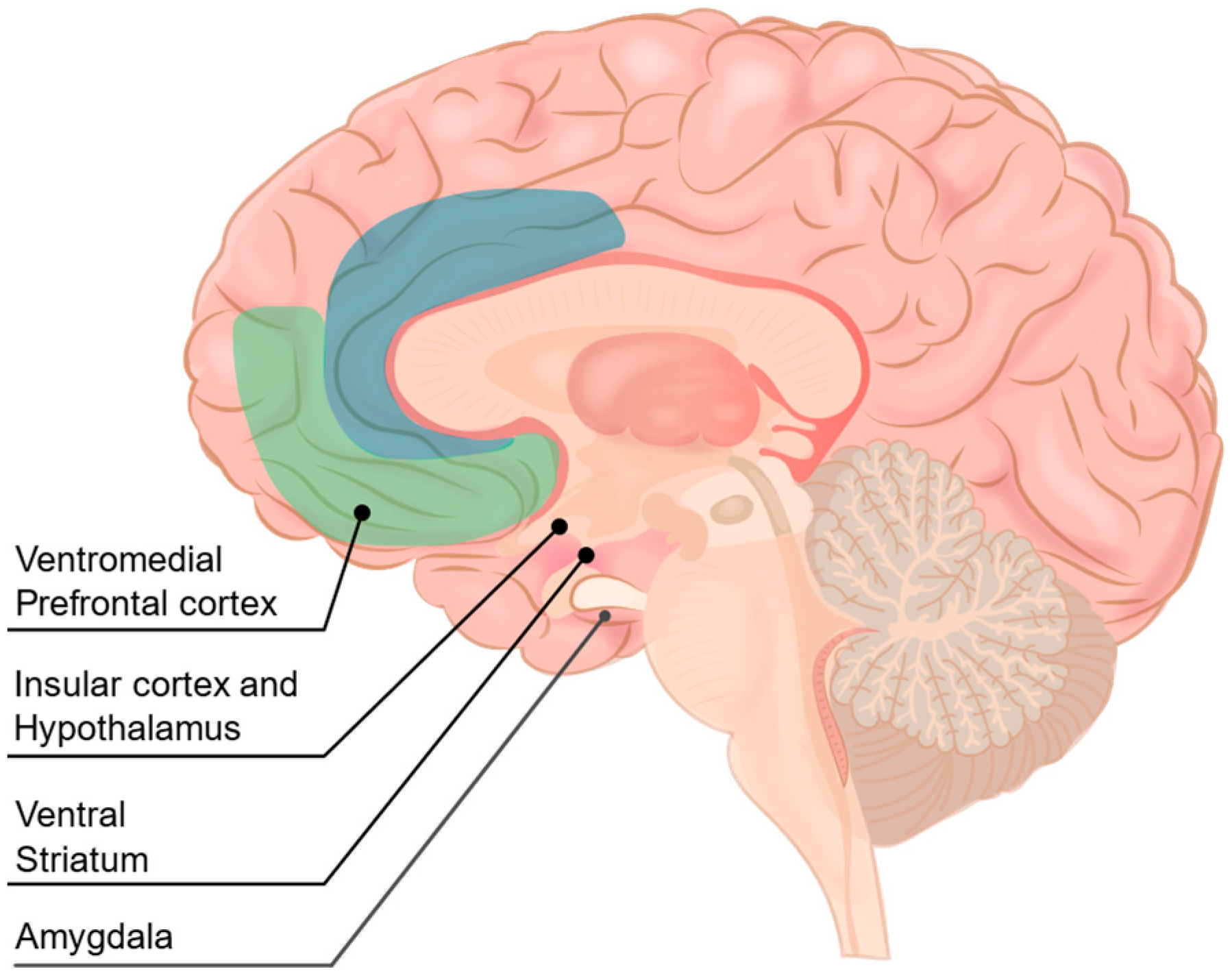
• The insular cortex and the hypothalamus—crucially involved in generating the autonomic components of emotions [9]. The human insular cortex is in the depth of the lateral fissure/Sylvian fissure and is connected to the amygdala and various limbic and association cortical areas [11]. Meanwhile, the hypothalamus is a small central structure located under the thalamus [12].
• The ventral striatum—plays a role in the execution of stereotyped emotional action patterns [9]. This structure is a ventral extension of the striatum and includes the nucleus accumbens [13].
• The ventromedial prefrontal cortex—plays a crucial role in controlling and inhibiting emotional responses considered socially unacceptable [9]. This region refers to the entire area of the prefrontal cortex, which is both ventral and medial [14].

According to Bericat (2016), emotions can essentially be classified into two types: primary and secondary. Primary emotions are considered universal, physiological, evolutionarily relevant, and innate from a biological and neurological point of view. Secondary emotions can result from a combination of primary emotions and are socially and culturally conditioned [15].

Robert Plutchik (1980s) stipulated a wheel that defines emotions (Figure 2), suggesting eight primary emotions: joy and sadness; anger and fear; trust and disgust; and surprise and anticipation [16]. These emotions can be expressed in different degrees of intensity, and there are three degrees for each. All human emotions can be formed through the combination of one or more of these basic emotions [17].

As mentioned above, emotions perform a crucial role in the daily lives of humans, and the need for and importance of recognising them automatically is being pushed by the growing interaction with computer systems that are gradually more human-like. Emotions can be identified through text, speech, facial expressions, gestures, and, more recently, electroencephalogram signals [17]. Changes in emotions can cause differences in these signals in terms of their frequencies and amplitudes, which will result in the manifestation of different emotional states [18].

1.3. Electroencephalography (EEG) and Its Assessement

EEG is a standard method for measuring brain activity over time in various domains using electrodes placed on the patient’s scalp [19]. The brain’s electrical activity is generated by electrical impulses resulting from communication between neurons and exhibits complex and significant behaviour, characterised by non-linear and dynamic properties [10,20]. These properties are intended to reflect the chaotic behaviour of the nervous system, like its complexity and stability [20]. Therefore, it has become the main source of signals for the development of non-invasive brain–computer interfaces (BCIs). These BCIs allow people to control devices through their brain activity, which can be relevant for individuals with motor difficulties [19].

EEG signals are generated by the postsynaptic potentials of cortical nerve cells, whether inhibitory or excitatory. These potentials add up in the cerebral cortex and propagate to the surface of the scalp, where they are picked up and recorded. A typical EEG signal has an amplitude that varies approximately between 10 and 100 µV, with a frequency in the range of 1 Hz to around 100 Hz [20]. In this signal, it is possible to identify distinct brain wave frequency ranges, namely, delta, theta, alpha, beta, and gamma waves, each associated with different mental states and cognitive functions [18].

Delta frequencies are normally between 0.5 and 3 Hz and their amplitude is around 20–200 μV. An EEG signal in this frequency band reflects a state of drowsiness and fatigue. On the other hand, theta frequencies are between 4 and 8 Hz and their amplitudes are approximately 10–50 μV, corresponding to stress situations [18]. Alpha frequencies are between 9 and 13 Hz with an amplitude of approximately 20–100 μV and are associated with relaxation [18,21]. Meanwhile, beta frequencies are between 14 and 30 Hz with amplitudes of around 5–20 μV and are indicative of excitation in the human brain. Finally, gamma frequencies vary above 31 Hz and are related to situations of great concentration and attention [18].

Although they are present in various regions of the brain, certain brain waves are characteristic of specific cortical parts. Therefore, to recognise emotions using EEG, it is important to understand the functions of the main parts of the human brain, which are represented in Figure 3, namely, the frontal, parietal, occipital, and temporal lobes (Figure 3) [18].

The frontal lobe includes all of the advanced features and controls human emotional expression and thought. The parietal lobe is associated with sensation and is responsible for perceiving tactile pressure, temperature, taste, and pain. The occipital lobe is the body’s visual processing centre and, finally, the temporal lobe is associated with memory and body movement [18].

Delta waves tend to occur mostly in the frontal region, especially in the frontal pole, while theta waves stand out in the temporal and parietal regions. Alpha waves occur especially in the occipital and parietal regions and beta waves are distinguished in the frontal region. On the contrary, the higher frequency waves, gamma waves, are not associated with any specific brain area because they do not follow a pattern and are in constant variation [22].

1.4. Problem

Emotions play a fundamental role in interactions and experiences. Therefore, understanding emotional signals becomes an important aspect that influences people’s communication through verbal and non-verbal behaviour. This understanding is relevant for healthcare professionals who deal with other people daily and make judgements about their physical and emotional state. For example, in a clinical context, expressions such as sadness and pain can signal suffering and the gravity of the problem and are relevant in doctor–patient communication [23]. However, scientific knowledge of these emotional states is still very limited [7]. The complexity and subjectivity of emotions make the process of perceiving them challenging. Emotions often do not manifest themselves in isolation, and people can experience a mixture of them [16]. In addition, some individuals may not express their emotions in a visible and perceptible way, as is the case with people with autism [24].

The inability to accurately perceive or interpret emotions can have serious consequences. In healthcare settings, a lack of understanding of a patient’s emotional state may lead to missed signs of distress, inadequate treatment, or a breakdown in communication, ultimately affecting patient outcomes. Beyond clinical contexts, this challenge extends to broader domains such as education, counselling, and human–machine interaction, where the ability to decode emotions can significantly enhance the quality of interactions.

When examining brain activity, the existing literature focuses on two primary aspects. First, it is crucial to identify which electrodes, corresponding to active brain regions, are associated with specific emotional states. Second, attention is directed toward the signal itself, aiming to determine which patterns correlate with particular emotions. From a computational perspective, especially within a machine learning framework, these aspects translate into identifying relevant features and selecting appropriate classification models. Together, these components create a broad and promising area of research that remains relatively underexplored, offering significant potential for advancements in emotion decoding and brain–computer interface applications.

1.5. Supporting Studies

In a study carried out by Zheng et al. (2014) with six subjects (three men and three women), EEG-based brain activity was measured using 12 emotional film extracts (6 positive and 6 negative), each lasting 4 min. The authors used machine learning methods to accurately read the subjects’ emotions and concluded that the characteristics of the high-frequency bands of brain activity, namely, beta and gamma, reflect emotional and cognitive processes [25].

Woaswi et al. (2016) inferred that facial expressions are not enough to describe or reveal an individual’s true emotions. However, analysing brain waves makes it possible to understand emotions more accurately and authentically, even when the individual is trying to hide them. The study used an unspecified group of participants and was based on the presentation of four videos, each 2 min long, which induced emotions such as anger, sadness, joy and surprise. The characteristics extracted from these stimuli were classified using artificial intelligence techniques aimed at interpreting emotional expression [26].

Ahmed et al. (2022) presented a deep learning approach for the automatic extraction of features for emotion classification based on EEG. This method uses a convolutional neural network (CNN) model for automatic feature learning, where features extracted from EEG data transformed into a two-dimensional feature vector known as an asymmetric map (AsMap) are introduced. This AsMap vector makes it possible to represent brain activity spatially, capturing the relationships between different regions of the brain during emotional experience. The study achieved a remarkable classification accuracy of 97.10% using the SJTU Emotion EEG Dataset (SEED) and 93.41% with the Dataset for Emotion Analysis using Physiological Signals (DEAP). In addition, the research emphasises the importance of the characteristics of the gamma band, which demonstrated superior classification accuracy compared to other frequency bands. It also investigates the impact of window size (length of time intervals used to segment EEG data for analysis) on classification performance, revealing that larger window sizes (e.g., 30 s) tend to result in a decrease in classification accuracy. This finding suggests that the temporal dynamics of emotional responses may be better captured with smaller window sizes (e.g., 3 s), allowing for more accurate feature extraction and classification [27].

Using CNNs, Donmez et al. (2019) carried out a study with the aim of classifying the EEG recordings of a group of 10 women, aged between 24 and 33, who were subjected to visual stimuli via a 224 s video. The authors classified three emotions using spectrogram images of EEG-stimulated signals as input for a CNN model: joy, sadness, and fear. It was concluded that fear represents a very dominant and intense emotion and was classified with a high success rate. The overall accuracy obtained using CNN to classify emotions was 84.69% [28].

Dabas et al. (2018) proposed a three-dimensional emotional model for classifying emotion based on the Valence–Arousal–Dominance (VAD) space. This model categorises emotions into eight distinct states: relaxation, tranquillity, boredom, disgust, nervousness, sadness, surprise, and excitement, each defined by specific combinations of valence, arousal and dominance. Using the DEAP dataset as input data, the research applied machine learning algorithms to classify emotions, such as Naive Bayes and SVM, achieving an accuracy of 78.06% and 58.90%, respectively [29].

Lastly, Kusumaningrum et al. (2020) developed an EEG-based emotion recognition system, consisting of a feature extraction subsystem and a classification subsystem, using the DEAP dataset. With this system, they obtained the highest recognition accuracy of 62.58% using the Random Forest method compared to other methods employed, such as SVM and k-NN, which showed lower results [30].

Table A1. Supporting studies.

Study	Data	Stimuli	Methods/Algorithms
EEG-based emotion classification using deep belief networks [26]	Obtained from 6 individuals (3 men and 3 women), each on two journeys at intervals of one week or more. Recorded using an ESI NeuroScan system from a 62-channel electrode cap.	12 emotional film extracts (6 positive and 6 negative), each 4 min long.	Using the algorithms DBN-HMM (Deep Belief Network-Hidden Markov Model), DBN (Deep Belief Network), GELM (Graph regularised Extreme Learning Machine), SVM (Support Vector Machine) and KNN (K-nearest neighbors)
Human Emotion Detection Via Brain Waves Study by Using Electroencephalogram (EEG) [27]	Obtained from an undefined group of individuals. Recorded by a CONTEC KT88-3200 32-channel encephalograph connected to an electrode cap.	4 2-min videos corresponding to anger, sadness, joy and surprise.	The extracted features were classified using artificial intelligence techniques for emotional faces.
Automated Feature Extraction on AsMap for Emotion Classification Using EEG [28]	Datasets SEED and DEAP in different classification problems based on the number of classes.	15 excerpts from Chinese films about 4 min long.	AsMap + CNN (Asymmetric Map + Convolutional Neural Network), DE (Differential Entropy), DASM (Differential Asymmetry), RASM (Relative Asymmetry) and DCAU (Differential Caudality)
Emotion Classification from EEG Signals in Convolutional Neural Networks [29]	Acquired from a group of 10 women aged between 24 and 33. Recorded by the Neurosky Mobile Mind-wave headset.	A specially edited video containing scenes of joy/fun, sadness and fear, lasting 224 s.	CNN (Convolutional Neural Network)
Emotion Classification Using EEG Signals [30]	Dataset DEAP	40 1-min music videos	Naïve Bayes, SVM
Emotion Recognition Based on DEAP Database using EEG Time-Frequency Features and Machine Learning Methods [31]	Dataset DEAP	40 1-min music videos	Random Forest, SVM, k-NN and Weighted k-NN

in Appendix A summarises the key aspects of each study mentioned, simplifying their comparison.

1.6. Objectives

Physiological signals are not influenced by subjective factors and can truly affect human emotional states. Therefore, emotion recognition based on physiological signals has many advantages in terms of reliability and practicality. Thus, the use of EEG, which evaluates spontaneous signals that are difficult to camouflage, plays a fundamental role in emotional research and identification [18].

In this context, to tackle the problem associated with the perception of emotions inherent in this study, the following objectives have been established: (1) to identify correlates of EEG patterns in the presence of a given emotion; (2) to observe the brain regions or electrodes that are most active/inactive in response to different emotional states; and (3) to test machine learning algorithms that can handle EEG signals and explore the parameter space to obtain maximum accuracy in classifying emotions.

2. Materials and Methods

2.1. Input Data

The present study used the DEAP dataset (Database for Emotion Analysis using Physiological Signals), which contains a set of data used for emotional analysis based on physiological signals such as the electroencephalogram (EEG), electromyogram (EMG), and electrocardiogram (ECG). The data analysed consisted of EEG and peripheral physiological signals from 32 healthy participants aged between 19 and 37 years (average 26.9 years), 50% of whom were women.

The data collection took place in a laboratory environment with controlled temperature and lighting, where everyone watched 40 videoclips from music videos lasting one minute. These video clips were selected from an initial sample of 120 (collected from the website last.fm), based on the subjective evaluation of volunteers who rated them on a discrete 9-point scale for valence, arousal and dominance. The 40 videos chosen had the highest ratings in terms of emotional strength and the least variation in responses. Subsequently, an affective highlighting algorithm selected the most effective segments for evoking emotions from each video, ensuring consistent and appropriate stimuli for the emotional analysis of the experiment.

The EEG was recorded at a sampling rate of 512 Hz, using 32 active AgCl electrodes (placed according to the international 10–20 system). Thirteen peripheral physiological signals were also recorded. In addition, for the first 22 of the 32 participants, a DV-quality video of the frontal face was recorded. The aim of capturing these videos is to allow the participants’ facial expressions to be analysed while watching the music videos. This helps to correlate the emotional responses expressed in the participants’ evaluations with physiological reactions and facial expressions, providing a more comprehensive understanding of the emotions induced by the stimuli. The dataset documentation does not provide an explanation as to why the frontal face video recording was conducted for only 22 out of the 32 participants, leaving this aspect unclear.

The experiment began with a two-minute baseline recording period, during which the participants visualised a fixation cross and were instructed to relax. Then, the 40 videos were shown over the course of 40 trials, each consisting of the following steps:

• Display of a 2 s information screen with the number of the current trial, to orientate participants on the progress of the experiment.
• Display of a 5 s recording of the baseline, presenting a fixation cross.
• Display of the selected music video, lasting 1 min.
• Self-assessment of arousal, valence, liking and dominance.

After 20 attempts, the participants took a short break, at which point the experimenter checked the quality of the signals and the placement of the electrodes, ensuring the continuity of the second part of the experiment. At the end of each trial, the participants made a self-assessment of their emotional reactions on specific scales: valence (ranging from unhappy or sad to happy or joyful), arousal (from calm or bored to stimulated or excited), dominance (ranging from submissive to dominant), and liking (measuring the participants’ personal tastes). Finally, after the experiment, the participants rated their familiarity with each song, using a scale from 1 (‘Never heard it before the experiment’) to 5 (‘Knew the song very well’) [31].

2.2. Methodology

During this project, a code was developed in the Python programming language to carry out a comprehensive analysis of the EEG data. It incorporates various signal processing methods and machine learning techniques to obtain relevant and well-founded conclusions about the problem in question.

The methodology used in this work was organised and visually represented using a block diagram, as shown in Figure 4. To achieve the main objective of the work, the procedure was divided into distinct stages, each with its own tasks and processes.

2.2.1. Data Preparation and Analysis

The input data were read to prepare them for analysis and to organise them into appropriate structures for training or evaluating the models. In this process, data were selected that only included the information relating to the brain activity of the first individual out of the 22 who had facial recordings available. This allowed for a more in-depth and detailed study of the data. Furthermore, as the aim was to identify irregularities or specific patterns of emotional response, analysing one individual made it easier to identify unique characteristics that could be missed in a more comprehensive analysis.

In this study, the characteristics extracted from the data corresponded to the signals coming from the Fp1, AF3, and F3 electrodes. These electrodes were considered due to their relevance for capturing electrical brain activity in the areas of the brain associated with emotional processing, offering specific and highly informative data. These areas of the brain have shown greater efficiency in emotional recognition compared to other channels, making them ideal for this type of analysis [32].

2.2.2. Irregularity Detection

Observing irregularities in brain responses over time in reaction to different emotional stimuli can help identify consistent patterns that associate brain activity with specific emotions. When an irregularity is observed recurrently in response to a certain type of emotional stimulus, this strengthens the evidence that this anomaly is related to the emotion in question. Thus, the participants’ brain responses were analysed, with an emphasis on identifying irregularities in the signals. To this end, the Histogram-based Outlier Score (HBOS) algorithm was applied. This algorithm evaluates each feature of the data set independently, generating one-dimensional histograms. HBOS is based on the principle that anomalies are rare events and should therefore have a low frequency in a histogram compared to common events [33]. Unlike distance-based methods, which rely on pairwise comparisons between data points, HBOS assumes independence between features, enabling it to handle high-dimensional datasets with greater computational efficiency. For this purpose, a histogram was created for each channel in the dataset. These histograms estimate the probability density function (PDF), dividing the range of values into discrete bins and calculating the frequency of observations within each bin. Then, the likelihood of a given data point belonging to the distribution was computed by referencing the bin corresponding to its feature value. The individual likelihood scores across channels were then combined to generate an overall outlier score for the data point.

One of HBOS’s key advantages is its computational simplicity. Since the histograms are computed independently for each feature, the method scales well to large datasets. This independence assumption makes HBOS particularly suitable for scenarios where features are only weakly correlated or uncorrelated. However, this assumption can also be a limitation, as it may not accurately capture relationships in datasets with significant feature interdependencies. Another important advantage of HBOS is its interpretability. The use of histograms allows for the straightforward visualisation of the feature distributions and provides insight into why certain points are classified as outliers. Additionally, HBOS can handle categorical and continuous data types by appropriately constructing histograms or equivalent frequency distributions.

2.2.3. Feature Extraction

The EEG data were processed considering the full one-minute recording dedicated to each independent video. For each recording, the power spectral density (PSD) was calculated, representing the power distribution of an EEG signal in the frequency domain [34]. In other words, this allowed the energy present in different frequency bands to be described, making it possible to identify the predominant ones in a signal at a given time and under certain conditions. In this context, its analysis is particularly useful for identifying the most active frequencies during emotional states. This is because different frequency bands (alpha, beta, delta and gamma) are associated with the above-mentioned emotional states. For this purpose, the periodogram method was used for the calculation.

Emotional states can be categorised based on different combinations of valence and arousal. Valence describes the degree to which an emotion is perceived as positive or negative, while arousal refers to the intensity of the associated emotional state. To record these characteristics, participants rated each video in terms of arousal and valence levels (on a discrete 9-point scale) [31]. The self-assessment of emotions made it possible to correlate the participants’ subjective perceptions of their emotional reactions to the videos with the objective data obtained from the EEG measurements. This helped validate the interpretations of the brain signals in relation to the emotions reported. The classification of the participants was then grouped into the 4 distinct categories described in

Table 1. Valence and arousal combinations.

Valence and Arousal Combinations	Emotional State
High arousal and high valence (HAHV)	Excited and happy
Low arousal and high valence (LAHV)	Calm and relaxed
High arousal and low valence (HALV)	Angry and nervous
Low arousal and low valence (LALV)	Sad and bored

.

Subsequently, topographic maps were developed using the Magnetoencephalography and Electroencephalography (MNE) framework (version 1.8.0). MNE-Python is an open-source software package that uses magnetoencephalography and electroencephalography signals to characterise and localise neuronal activation in the brain. This package covers a variety of methods, including data pre-processing, source localisation, statistical analysis and the estimation of functional connectivity between distributed brain regions [35]. These maps have been used to observe the most active/inactive brain regions and compare the activity of different frequency bands during the expression of emotions.

It is important to note that before the topographic maps were constructed, an FIR (Finite Impulse Response) filter was applied. The filter’s bandwidth was adjusted to allow only the frequencies corresponding to each band of interest to pass through, blocking out the others. In this way, it was possible to isolate specific frequency bands (alpha, beta, theta and gamma), making it easier to compare brain activity in different emotional states. Attenuation is 53 dB in the rejection band, which means that signals outside the desired range are drastically reduced, avoiding interference. In addition, the filter’s phase response is linear, which means that all frequencies within the chosen range are delayed evenly in time. This is crucial, as it preserves the original shape of the signal, ensuring that the analysis of brain activity is accurate and reliable.

2.2.4. Emotion Classification Task

To estimate emotional states using the EEG data studied, classification prediction algorithms such as Support Vector Machine (SVM), Multi-Layer Perceptron (MLP) and Random Forest (RF) were used. These algorithms are designed to identify patterns in the training data by analysing the brain signals across different frequency ranges and specific brain regions. Based on the patterns extracted, they can predict levels of valence (positive or negative emotions) and arousal (degree of intensity of the emotion). Based on the dataset annotation, where valence and arousal are rated on a 1 to 9 scale, binarised labels were attributed, considering 1–4 as Low and 5–9 as High, for both variables. The distribution of High and Low classes across the dataset is approximately balanced.

SVM is a supervised machine learning algorithm that uses machine learning theory to maximise prediction accuracy while avoiding overfitting to the data. By employing an approach that aims to find the best separation between different classes in the feature space, it demonstrates effectiveness in dealing with large datasets [36]. The used SVM classifier was configured with a linear separation type (kernel), which allows the data to be divided with a single straight line. The regulation parameter (C), which controls the balance between the separation margin and the correct classification of the training points, was kept at the default value of 1.0. In addition, the probability estimation option was activated, providing additional information on the confidence of the predictions made. The input size is defined by the number of features in the dataset used during training.

The MLP is a feedforward neural network that uses the backpropagation technique for learning. This network is made up of an input layer of neurons, which act as receivers; one or more hidden layers of neurons, which compute the data and undergo iterations; and the output layer, which predicts the output [37]. For the model to learn efficiently, we used the Adam method, a stochastic gradient-based optimiser that dynamically adjusts the weights (strength of the connections between neurons) during training, making it more effective. In addition, the tanh (hyperbolic tangent) activation function was used in all the hidden layers, which helps to introduce non-linearities into the model, improving its ability to learn complex patterns. Another relevant adjustment was the alpha parameter, set to a value of 0.3, which helps to avoid overfitting the training data, ensuring that the model continues to perform well with new data. In addition, the model was trained for up to 400 iterations to improve the accuracy and quality of the model’s predictions. As far as the architecture is concerned, the standard configuration was maintained, with a single hidden layer containing 100 neurons. The input size was defined by the number of features present in the training data.

The RF algorithm involves building multiple decision trees during the training of the model and combining them to obtain a more robust and generalised prediction. To classify a new instance with this model, after training the forest, it goes through all of the defined decision trees that contribute their own prediction. In the end, the contributions of each tree (counted as votes) are totalled and the class that receives the most votes is chosen as the final prediction [38]. The number of independent decision trees in the forest was set at 100. The splitting metric used was ‘gini’, which helps decide how to split the data at each node of the tree to maximise the purity of the splits. The maximum depth of the trees was left unrestricted, allowing them to grow to the maximum possible limit, which can help capture more detail in the data.

2.2.5. Statistical Analysis

To corroborate the conclusions drawn from the topographical maps, a statistical analysis was carried out using the Mann–Whitney test. This non-parametric test is suitable for assessing whether there are significant differences between two groups, without assuming that the data follow a specific distribution [39]. The analysis was conducted in two stages, with the first centred on assessing the variation in frequency bands over time, and the second on comparing brain activity between the different frequency bands and brain regions. This approach provided a solid statistical basis for the interpretations of the variations in brain activity associated with the different emotional states analysed.

The performance of each classification algorithm can vary depending on the specific characteristics of the dataset and the task in question. The choice of algorithm involves testing and fine-tuning to obtain the best results for a given problem. To assess the performance of these algorithms, K-fold cross-validation was carried out. This technique splits the dataset into a training set and a test set several times, training and testing the model on different subsets [40]. In this way, a more reliable estimate of the model’s performance is obtained.

In this study, a 5-fold cross-validation approach was used. This method divides the dataset into 5 equal parts (folds), ensuring that each fold serves as the test set exactly once while the remaining 4 folds are used for training the model. This process is repeated across 5 iterations, resulting in a comprehensive evaluation of the model’s performance. Cross-validation is crucial because it prevents the model from overfitting, i.e., memorising the training data, and ensures it generalises well to unseen data. A ratio of 70% for training and 30% for testing was chosen in order to balance the trade-off between learning and evaluation. Allocating 70% of the data for training provides the model with a sufficient amount of information to learn from, while reserving 30% for testing ensures a reliable and representative evaluation of its performance. An inadequate split can lead to overfitting, where the model performs well on training data but fails to generalise to new data. Bearing in mind that, when running the code several times, the results may change somewhat due to, for example, splitting the data into different training and test sets, the cross-validation process was repeated 10 times and then the average of the accuracy and F1 scores obtained were calculated, as well as the standard deviations of the results. This combined approach of cross-validation and repeated evaluations provides confidence in the reported results by ensuring they are not dependent on a single random split of the data. It reflects the model’s ability to generalise across diverse data configurations, which is essential for assessing its real-world applicability.

Using these results, the algorithm with the best performance in the first validation was identified, i.e., the one with the highest accuracy and F1 score in classifying valence and excitation for different combinations of frequency bands and brain regions. A second cross-validation was then carried out for this specific algorithm, where the accuracy and F1 score were calculated, allowing for a more rigorous and detailed assessment of its performance. Confusion matrices were also constructed to assess performance, consisting of a square matrix of numbers expressing the number of sample units associated with a given category during the classification process carried out, and the real category to which these units belong [41].

It should be noted that selecting the right characteristics of the EEG signals is crucial in identifying the most relevant information for a given predictive model. This can be achieved by eliminating redundant variables and selecting those that best distinguish between classes. In addition, to obtain better results for the various parameters evaluated, it is necessary to optimise the classification process by exploring the parameter space. In this way, by reducing data dimensionality and the complexity of the model, it is possible to promote greater computational efficiency and accuracy of the results, leading to a more portable system that is easier to implement, for example, in a neurowearable device.

3. Results

The EEG signals were analysed in several stages, starting with the detection of possible irregularities in the data that could indicate the presence of emotions. The graph in Figure 5 illustrates the irregularities identified in the first 1000 s, according to the training model obtained by pre-processing the input data. In this graph, the reddish line indicates the regions where the model detected possible emotions, while the blue line represents the areas considered normal.

Afterwards, periodograms were calculated using the Welch method, which makes it possible to estimate the power associated with each frequency in a signal spectrum. This method involves dividing the signal into segments, obtaining the modified periodogram of these segments and the average of these modified periodograms [42]. In order to extract specific characteristics of the EEG signal, Welch’s method was applied to the three electrodes under study, as illustrated in Figure 6.

In this way, it was possible to analyse the power spectral density for each characteristic EEG band, namely, the theta, alpha, beta, and gamma bands, as shown in Figure 7. The spectral density range corresponding to each frequency band is shaded in blue, highlighting the intervals under analysis and providing a visual distinction of the activity within each band. It should be noted that although only the graphs corresponding to the FP1 electrode are shown, the same procedures were applied to the AF3 and F3 electrodes.

Figure 8 shows the classifications of the 40 videos watched by an individual, based on two important emotional components: valence and arousal.

The selected participant’s responses were organised into the four categories described in Table 1. For each of these categories, the mean and standard deviation of the evaluations obtained were calculated. The results are presented graphically in Figure 9 and numerically in

Table 2. Statistical analysis of valence and arousal combinations: comparison of mean and standard deviation across categories (HAHV, LAHV, HALV, LALV).

	HAHV	LAHV	HALV	LALV
Average valence ± Standard deviation	7.12 ± 1.04	6.67 ± 1.09	3.19 ± 1.23	3.57 ± 1.12
Average arousal ± Standard deviation	6.81 ± 0.84	3.87 ± 1.09	6.79 ± 0.96	3.47 ± 1.19

.

Following this, topographic maps of each brain wave were developed in the time interval from 0.05 to 0.251 s. During this interval, a fixation cross was presented to the participant, who was asked to relax during this period. In this way, the brain’s initial response to visual or auditory stimuli was captured, which is crucial to understanding how the brain processes and reacts to new stimuli and emotional states. Additionally, focusing on a specific and relatively short interval can help reduce variability in the data. Figure 10, Figure 11, Figure 12 and Figure 13 show the topographic maps for the theta, alpha, beta and gamma waves, respectively.

Additionally, it should be noted that, based on the analysis of Figure 7, the delta wave, whose frequency varies between 0.5 and 3 Hz, has a low or even non-existent amplitude in the PSD. This suggests that the frequencies associated with these waves do not show significant activity in the expression of emotional states during signal analysis. Furthermore, delta waves are typically related to states of drowsiness, as discussed above. Given that the experiment was conducted with fully awake participants, an analysis of the delta waves was not carried out, since their relevance in emotional contexts is limited under these conditions.

Subsequently, Figure 14, Figure 15, Figure 16 and Figure 17 were developed, illustrating topographical maps of the different frequency bands (theta, alpha, beta, and gamma) associated with each valence and excitation classification: HAHV, HALV, LAHV, and LALV, respectively, at a time of 0.15 s.

Statistical Analysis

The graphs in Figure 18 show the results of the statistical analysis carried out on the topographic maps in Figure 14, Figure 15, Figure 16 and Figure 17, which compare brain activity in different frequency bands and brain regions.

Table 3. Comparative statistical analysis of brain activity between different frequency bands and brain regions. (p-values based on the Mann-Whitney test; comparisons with 95% confidence interval are represented in bold face).

		HALV			HAHV			LALV			LAHV
		Alpha	Beta	Gamma	Alpha	Beta	Gamma	Alpha	Beta	Gamma	Alpha	Beta	Gamma
Frontal	Theta	<0.001	0.009	<0.001	<0.001	0.014	<0.001	0.885	0.006	0.010	0.371	0.751	0.707
	Alfa		<0.001	<0.001		<0.001	0.001		<0.001	<0.001		0.312	0.583
	Beta			<0.001			<0.001			<0.001			0.665
Central	Theta	0.180	0.394	0.485	0.093	0.937	0.065	0.240	0.310	1.000	0.026	0.589	0.310
	Alfa		0.180	0.394		0.009	0.589		1.000	0.240		0.310	0.180
	Beta			0.818			0.009			0.394			0.699
Temporal	Theta	0.667	1.000	0.667	1.000	1.000	1.000	1.000	1.000	1.000	0.333	1.000	0.333
	Alfa		0.667	1.000		0.667	1.000		1.000	0.667		0.333	1.000
	Beta			0.667			0.667			1.000			0.333
Parietal	Theta	0.026	0.240	0.132	0.002	0.132	0.002	1.000	0.394	0.589	0.002	0.132	0.065
	Alfa		0.065	0.132		0.002	0.009		0.589	0.180		0.394	0.065
	Beta			0.394			0.002			0.240			1.000
Occipital	Theta	0.333	0.333	0.333	0.333	0.333	0.333	0.667	0.667	0.667	0.333	0.667	0.333
	Alfa		0.333	0.333		0.333	0.333		0.667	0.667		0.333	0.667
	Beta			0.333			0.333			0.667			0.667

summarises the p-values generated by the statistical analysis (carried out using the Mann-Whitney test), evaluating the relationship between the brain activity of different waves and the corresponding brain regions.

The performance of the three machine learning algorithms (SVM, MLP and RF) in classifying valence and excitation using different combinations of frequency bands and brain regions was evaluated based on the average accuracy and the average F1 score, both accompanied by their respective standard deviations. The results obtained for the performance of the three algorithms for excitation and valence are shown in

Table 4. Statistical analysis of arousal state classification: Comparison of average accuracy, F1 score, and standard deviation across algorithms (SVM, MLP, RF).

	SVM	MLP	RF
Average accuracy ± Standard deviation	0.5931 ± 0.0364	0.5972 ± 0.0321	0.5772 ± 0.0273
Average F1 score ± Standard deviation	0.6458 ± 0.0388	0.6354 ± 0.0435	0.5899 ± 0.0398

and

Table 5. Statistical analysis of valence state classification: Comparison of average accuracy, F1 score, and standard deviation across algorithms (SVM, MLP, RF).

	SVM	MLP	RF
Average accuracy ± Standard deviation	0.5775 ± 0.0367	0.5989 ± 0.0399	0.6270 ± 0.0324
Average F1 score ± Standard deviation	0.5852 ± 0.0360	0.6278 ± 0.0359	0.6514 ± 0.0354

, respectively.

Based on the data in Table 4, it can be seen that the algorithm with the best performance, considering the average values, was the MLP, while the SVM obtained the best F1-score in the arousal states. On the other hand, the data in Table 5 shows that the RF algorithm performed best in terms of both the average and the F1-score when defining valence emotional states.

Table 6. Valence accuracy with the RF algorithm.

	Left	Frontal	Right	Central	Parietal	Occipital
Theta	51.22	51.22	60.16	60.98	52.03	52.03
Alpha	59.35	56.91	54.47	59.35	55.28	60.16
Beta	63.41	58.54	55.28	59.35	63.41	57.72
Gamma	56.10	65.85	56.10	60.98	62.60	60.16

,

Table 7. Arousal accuracy with the MLP algorithm.

	Left	Frontal	Right	Central	Parietal	Occipital
Theta	43.09	53.66	50.41	56.10	56.10	57.72
Alpha	51.22	53.66	53.66	55.28	54.47	47.97
Beta	52.85	50.41	52.03	47.97	52.85	51.22
Gamma	60.98	54.47	47.97	59.35	55.28	56.10

,

Table 8. F1 score of valence with the RF algorithm.

	Left	Frontal	Right	Central	Parietal	Occipital
Theta	58.82	58.06	59.02	63.38	60.00	50.82
Alpha	55.71	62.60	63.70	54.84	50.77	56.72
Beta	63.16	55.17	55.74	49.18	51.97	46.28
Gamma	68.25	66.67	58.91	66.07	67.69	65.12

and

Table 9. F1 score of arousal with the SVM algorithm.

	Left	Frontal	Right	Central	Parietal	Occipital
Theta	69.41	62.65	69.46	69.36	67.90	67.03
Alpha	64.24	56.44	71.51	65.12	67.95	69.27
Beta	26.37	67.07	67.05	64.74	61.73	65.52
Gamma	25.29	60.82	63.22	65.54	20.00	66.29

show the results, in percentages, for the accuracy of valence and arousal with the RF and MLP algorithms, respectively, and the F1 scores for valence with the RF algorithm and arousal with the SVM algorithm.

Lastly, based on the results obtained, confusion matrices were constructed for the algorithm with the best performance in classifying valence and excitation, considering each combination of frequency band and brain region. Figure 19 illustrates confusion matrices that assess the RF algorithm’s performance in predicting valence labels for the theta wave in the central region of the brain, the beta wave in the frontal region, the gamma wave in the parietal region and the alpha wave in the occipital region. These matrices make it possible to visualise the performance of the classification model, categorising the predictions into true positives (TP), true negatives (TN), false positives (FP) and false negatives (FN). Each of these categories is represented by a specific cell within the confusion matrix, making it easier to analyse the results of the model in detail [41,43].

Figure 20 shows the confusion matrices that analyse the MLP algorithm’s performance in predicting arousal labels, as was done for valence.

4. Discussion

This research presents a detailed analysis of the relationship between the brain’s electrical activity and human emotions, using EEG data to investigate how different emotional states manifest themselves in brain wave patterns. The analysis began by applying the HBOS method. As illustrated in Figure 5, HBOS can be a useful tool for exploring the data, due to its ability to detect possible irregularities that may indicate the presence of emotions. However, it is important to emphasise that HBOS alone is not enough to classify emotions directly and accurately. It is therefore necessary to adopt other approaches to enable a more detailed analysis.

The evaluation of the periodograms shown in Figure 7, carried out to identify the most active frequencies during emotional states, showed a lower power spectral density for the gamma wave, as well as the presence of a peak in the beta wave frequency range. The identification of peaks at certain frequencies suggests the existence of oscillations or recurring patterns in the data.

These emotional states can be characterised by the interaction of valence and excitation components, as shown in Figure 8. From this, it is possible to highlight the fact that high valence is associated with positive emotions and high arousal is related to a more intense emotional state, and vice versa.

Topographic maps of brain activity use colours to represent the intensity of electrical activity in different areas of the brain, measured in microvolts. Regions highlighted with warmer colours, such as red or orange, indicate more intense electrical activity compared to other areas. This visual representation makes it possible to intuitively identify the areas of the brain with the greatest activation of specific waves. Analysing Figure 10, which illustrates the topographical map obtained for the theta wave, a greater activity can be seen in the occipital region of the brain (Mann-Whitney test, p-value = 0.023), which may indicate that the brain is carrying out visual processing. In the context of analysing emotions, a lower prevalence of the theta wave may suggest a greater influence of more relaxed states during the period examined. The activity of the theta wave is notoriously variable over time. This variation can be attributed to the different intensities and durations of stress that the individual experiences or to their level of fatigue. The reduction in cognitive capacity and performance associated with fatigue is often related to an increase in the overall power of the theta waves [44].

The alpha wave map shown in Figure 11 reveals the variation in their activity over time, being possible to identify variations in the temporal areas with a significance near meaningful values (Mann-Whitney test, p-value = 0.058). These can be attributed to differences in stress and fatigue levels that can be characterised by a lower degree of relaxation where alpha activity tends to decrease. On the other hand, fatigue can result in an increase in alpha activity, reflecting changes in the individual’s mental state [44].

Figure 12 and Figure 13 show the maps for beta and gamma waves, respectively, where no statistical significance was identified. In the first figure, there is a greater predominance of activity in the frontal region, while in the second, the most active region is the parietal, which is in line with what has been described in the literature. In both, there are no observable changes over time, indicating that there is no variation in cognitive activity and concentration during the visualisation of the musical excerpts.

Analysing Figure 14, which depicts the HAHV emotional state, reveals a high level of beta wave activity in the frontal region of the brain compared to theta waves (Mann-Whitney test, p = 0.031). This was to be expected, as they are associated with arousal in the human brain. In addition, a decrease in theta waves compared to alpha waves was observed in this region (Mann-Whitney test, p = 0.000), which may indicate states of reduced stress. There was also a decrease in alpha and theta wave activity in the parietal region compared to the gamma wave (Mann-Whitney test, p = 0.009 and p = 0.002, respectively), which may indicate greater concentration and less relaxation and stress.

In the HALV emotional state, illustrated in Figure 15, there is a significant decrease in alpha activity in the frontal region compared to the gamma and theta waves (Mann-Whitney test, p-values of 0.002 and 0.000 respectively), which reinforces the idea of a state of high attention accompanied by less relaxation. In contrast, in the calm and relaxed state (LAHV), shown in Figure 16, there is an increase in the theta wave compared to the alpha waves in the central and parietal regions of the brain (Mann-Whitney test, p-values of 0.026 and 0.002 respectively), which may reflect a state of introspection.

In emotional states associated with sadness and boredom (LALV), there is a decrease in beta wave activity in the frontal region of the brain compared to alpha and theta waves (Mann-Whitney test, p-values of 0.002 and 0.031 respectively), which indicates a lack of brain arousal. It can also be related to introspection, deep reflection and a tendency to relax. In addition, a decrease in the gamma wave compared to the alpha and theta waves is observed in the same region (Mann-Whitney test, p-values of 0.003 and 0.045 respectively), which reflects a reduction in attention and intense cognitive processing. These observations are illustrated in Figure 17.

Based on the statistical analysis applied to the topographical maps (Figure 18 and Table 3), it can be said that the emotional states HALV, HAHV and LALV allow for clear distinctions in the frontal region, especially in the theta wave. Furthermore, in the parietal region it is possible to observe statistical significance between the theta and alpha waves, except in the case of the LALV state. It is also important to emphasise that the LAHV state was the one with the lowest number of statistical results supporting definitive conclusions.

With regard to the statistical analysis carried out, the metrics adopted provide a comprehensive view of the classifiers’ performances, reflecting both the overall precision of the models (accuracy) and the ability to balance precision and recovery (F1 score). The standard deviation, in turn, indicates the variability of the results in different runs or experimental conditions, providing an assessment of the consistency of the models’ performance. Once the best algorithms had been selected, the same metrics were evaluated, but to classify valence and arousal in different combinations of frequency bands and brain regions. This was done in order to conclude which brain regions are most influential in each type of EEG wave. Thus, by identifying the most relevant characteristics, the models can be adjusted to improve the accuracy of predictions and become more efficient.

Finally, when analysing the confusion matrices in Figure 19, it can be seen that the RF algorithm performed better for the gamma wave in the parietal region. This is due to the fact that it classified the valence correctly in a greater number of cases, considering the ratio of correct classifications to the total. In the confusion matrices in Figure 20, it is clear that the MLP algorithm showed better results for the alpha wave in the occipital region, as it classified the arousal correctly in more cases.

5. Conclusions

5.1. Main Contributions

This study contributes to the advancement of emotion recognition by exploring the relationship between EEG signals and emotional states. By investigating how emotions can be objectively identified, the work highlights the importance of analysing physiological data in understanding human emotional complexities. In particular, by focusing on specific electrodes (Fp1, AF3, F3), and employing advanced techniques such as Welch’s Method for power spectrum estimation and Histogram-Based Outlier Score (HBOS) for irregularity detection, it has been shown how to improve the accuracy and reliability of emotion detection systems. These methodological innovations contribute to the development of more robust and precise emotion recognition models.

In addition, the work integrates machine learning techniques into emotional classification, offering significant potential for improving human-machine interaction systems. This methodological advance could have practical applications in various areas, such as mental health, where the accurate identification of emotional states is essential for more personalised and effective interventions.

The real-time emotional monitoring enabled by accurate emotion detection could be instrumental in assessing patient discomfort or anxiety during medical procedures, such as surgeries, allowing for timely interventions. Furthermore, emotion recognition systems could be integrated into mental health care, offering real-time emotional feedback that could lead to more personalised and adaptive treatment strategies.

The proposed system contributes to provide a deeper understanding of the EEG, highlighting it as a valuable tool in the detection of emotions, offering insights into the brain activity associated with different emotional states. This problem proves crucial in the field of Biomedical Engineering, where understanding the interactions between the brain and emotions is fundamental to the development of innovative biomedical applications, therapies and interventions. For example, it can be used in the diagnosis of illnesses such as depression, since it is characterised by a slight arousal of the brain, and in the perception of discomfort when performing medical surgery.

Furthermore, this study contributes to the development of more accessible and practical EEG devices by demonstrating that emotion detection can be effectively achieved with fewer electrodes. The use of fewer electrodes offers several advantages, such as increased comfort for users, reduced equipment complexity, and lower device costs. This simplification can facilitate the implementation of emotional monitoring systems in various settings, including clinics, hospitals, and even personal devices, expanding the accessibility and applicability of the technology. Moreover, fewer electrodes can enhance patient acceptance, as the reduced number of sensors makes the system less invasive, thus providing a more comfortable experience, particularly in medical contexts.

Finally, by studying the categorisation of emotions, this study paves the way for future research and contributes to the development of adaptive emotional technologies, promoting a deeper understanding of human emotions and their impact on behaviour.

5.2. Comparative Study

For a comprehensive comparison, several scenarios with various conditions have been assessed, described in

Table 10. Comparison between the proposed method and related works.

Study	Classifiers	Parameters	Training/Testing Conditions	Average Accuracy (%)
Ahmed et al. (2022) [28]	AsMap + CNN (Asymmetric Map + Convolutional Neural Network), DE (Differential Entropy), DASM (Differential Asymmetry), RASM (Relative Asymmetry) and DCAU (Differential Caudality)	For AsMap + CNN: 3 × 3 kernel, ReLU activation.	Not specified	97.10% (with SEED) 93.41% (with DEAP)
Donmez et al. (2019) [29]	CNN (Convolutional Neural Network)	Not specified	80/20% split for training/testing (392/98 images). Trained with 20 epochs and 26 iterations per epochs.	84.69%
Dabas et al. (2018) [30]	Naïve Bayes, SVM	Not specified	Not specified	78.06% (Naïve Bayes) 58.90% (SVM)
Kusumaningrum et al. (2020) [31]	Random Forest, SVM, k-NN and Weighted k-NN	For RF: 100 trees. For SVM: linear kernel. For k-NN and Wk_NN: k = 7.	5-fold cross-validation	62.58% using Random Forest (highest recognition accuracy compared to other methods employed)
This study	RF	100 trees and ‘gini’ as the splitting metric.	70/30% split for training/testing	Arousal: 57.72% Valence: 62.70%
	SVM	Linear kernel.		Arousal: 59.31% Valence: 57.75%
	MLP	‘tanh’ activation, alpha = 0.3, 400 iterations.		Arousal: 59.72% Valence: 59.89%

.

Compared to the results presented by Kusumaningrum et al. (2020) [31], this study demonstrated superior performance in classifying valence using the RF algorithm. Furthermore, comparison with other studies suggests that there is potential for further optimisation, despite the distinct study conditions.

5.3. Limitations and Future Work

The positioning of EEG electrode, even when performed by an experienced professional, can vary slightly. Bearing in mind that the accurate interpretation of brain topographic maps requires careful consideration of the experimental context, data collection methods and individual characteristics, this proved to be a potential limitation.

Regarding future work, we recommend taking dominance into account as an emotional component, as mentioned in a study by Dabas et al. [30], in order to obtain a more detailed set of emotional states. Another suggestion would be to implement a Long Short-Term Memory (LSTM) or Gated Recurrent Unit (GRU) neuronal network to process the brain signals, offering a more detailed analysis of the temporal dynamics of emotional responses. In addition, it is proposed to carry out a comparison between the data taken from the dataset and values obtained in the laboratory. This comparison would be essential to understand whether the code implemented, and the models used fit different experimental data. It is also recommended to carry out a comprehensive analysis that considers the data of all individuals, using the average of the results as a basis, rather than focusing exclusively on the data of a single participant. Finally, comparison with the facial expressions recorded during the experiment can enrich the interpretation, providing a more detailed and accurate understanding of the results obtained.

References

1. Nonweiler, J.; Vives, J.; Barrantes-Vidal, N.; Ballespí, S. Emotional self-knowledge profiles and relationships with mental health indicators support value in ‘knowing thyself’. Sci. Rep. 2024, 14, 7900. [Google Scholar] [CrossRef]
2. Aballay, L.N.; Collazos, C.A.; Aciar, S.V.; Torres, A.A. Analysis of Emotion Recognition Methods: A Systematic Mapping of the Literature. In International Congress of Telematics and Computing; Springer Nature: Cham, Switzerland, 2024; pp. 298–313. [Google Scholar] [CrossRef]
3. Misselhorn, C.; Poljanšek, T.; Störzinger, T.; Klein, M. (Eds.) Emotional Machines; Springer Fachmedien: Wiesbaden, Germany, 2023. [Google Scholar] [CrossRef]
4. Spezialetti, M.; Placidi, G.; Rossi, S. Emotion Recognition for Human-Robot Interaction: Recent Advances and Future Perspectives. Front. Robot. AI 2020, 7, 532279. [Google Scholar] [CrossRef] [PubMed]
5. Hattingh, C.J.; Ipser, J.; Tromp, S.A.; Syal, S.; Lochner, C.; Brooks, S.J.; Stein, D.J. Functional magnetic resonance imaging during emotion recognition in social anxiety disorder: An activation likelihood meta-analysis. Front. Hum. Neurosci. 2013, 6, 347. [Google Scholar] [CrossRef]
6. Coelho, L. Speech as an Emotional Load Biomarker in Clinical Applications. Med. Interna 2024, 31, 7–13. [Google Scholar]
7. Suhaimi, N.S.; Mountstephens, J.; Teo, J. EEG-Based Emotion Recognition: A State-of-the-Art Review of Current Trends and Opportunities. Comput. Intell. Neurosci. 2020, 2020, 8875426. [Google Scholar] [CrossRef] [PubMed]
8. Li, M.; Lu, B.-L. Emotion classification based on gamma-band EEG. In Proceedings of the 2009 Annual International Conference of the IEEE Engineering in Medicine and Biology Society, Minneapolis, MN, USA, 3–6 September 2009; pp. 1223–1226. [Google Scholar] [CrossRef]
9. Gainotti, G. ENS TEACHING REVIEW Disorders of emotional behaviour. J. Neurol. 2001, 248, 743–749. [Google Scholar] [CrossRef]
10. Bellani, M.; Baiano, M.; Brambilla, P. Brain anatomy of major depression II. Focus on amygdala. Epidemiol. Psychiatr. Sci. 2011, 20, 33–36. [Google Scholar] [CrossRef]
11. Nieuwenhuys, R. The insular cortex: A review. Prog. Brain Res. 2012, 195, 123–163. [Google Scholar] [CrossRef] [PubMed]
12. Baloyannis, S.; Gordeladze, J. (Eds.) Hypothalamus in Health and Diseases; BoD–Books on Demand: London, UK, 2018. [Google Scholar]
13. Park, Y.-S.; Sammartino, F.; Young, N.A.; Corrigan, J.; Krishna, V.; Rezai, A.R. Anatomic Review of the Ventral Capsule/Ventral Striatum and the Nucleus Accumbens to Guide Target Selection for Deep Brain Stimulation for Obsessive-Compulsive Disorder. World Neurosurg. 2019, 126, 1–10. [Google Scholar] [CrossRef] [PubMed]
14. Bhanji, J.; Smith, D.; Delgado, M. A Brief Anatomical Sketch of Human Ventromedial Prefrontal Cortex. PsyArXiv 2019. [Google Scholar] [CrossRef]
15. Bericat, E. The sociology of emotions: Four decades of progress. Curr. Sociol. 2016, 64, 491–513. [Google Scholar] [CrossRef]
16. Chafale, D.; Pimpalkar, A. Review on developing corpora for sentiment analysis using plutchik’s wheel of emotions with fuzzy logic. Int. J. Comput. Sci. Eng. 2014, 2, 14–18. [Google Scholar]
17. Liu, Y.; Sourina, O.; Nguyen, M.K. Real-Time EEG-Based Emotion Recognition and Its Applications. In Transactions on Computational Science XII: Special Issue on Cyberworlds; Springer: Berlin/Heidelberg, Germany, 2011; pp. 256–277. [Google Scholar] [CrossRef]
18. Liu, H.; Zhang, Y.; Li, Y.; Kong, X. Review on Emotion Recognition Based on Electroencephalography. Front. Comput. Neurosci. 2021, 15, 758212. [Google Scholar] [CrossRef] [PubMed]
19. Müller-Putz, G.R. Electroencephalography. Handb. Clin. Neurol. 2020, 168, 249–262. [Google Scholar] [CrossRef] [PubMed]
20. Subha, D.P.; Joseph, P.K.; Acharya, U.R.; Lim, C.M. EEG signal analysis: A survey. J. Med. Syst. 2010, 34, 195–212. [Google Scholar] [CrossRef]
21. Crabbe, J.B.; Dishman, R.K. Brain electrocortical activity during and after exercise: A quantitative synthesis. Psychophysiology 2004, 41, 563–574. [Google Scholar] [CrossRef]
22. Groppe, D.M.; Bickel, S.; Keller, C.J.; Jain, S.K.; Hwang, S.T.; Harden, C.; Mehta, A.D. Dominant frequencies of resting human brain activity as measured by the electrocorticogram. Neuroimage 2013, 79, 223–233. [Google Scholar] [CrossRef] [PubMed]
23. Adriano, T.; Arriaga, P. Exaustão emocional e reconhecimento de emoções na face e voz em médicos. Psicol. Saúde Doenças 2016, 17, 97–104. [Google Scholar] [CrossRef]
24. Santos, P.A.R.D. Rastreamento Virtual da Face: Um Sistema Para Espelhar Emoções. Master’s Thesis, Universidade do Minho, Braga, Portugal, 2019. [Google Scholar]
25. Zheng, W.-L.; Zhu, J.-Y.; Peng, Y.; Lu, B.-L. EEG-based emotion classification using deep belief networks. In Proceedings of the 2014 IEEE International Conference on Multimedia and Expo (ICME), Chengdu, China, 14–18 July 2014; pp. 1–6. [Google Scholar] [CrossRef]
26. Ismail, W.O.A.S.W.; Hanif, M.; Mohamed, S.B.; Hamzah, N.; Rizman, Z.I. Human Emotion Detection via Brain Waves Study by Using Electroencephalogram (EEG). Int. J. Adv. Sci. Eng. Inf. Technol. 2016, 6, 1005. [Google Scholar] [CrossRef]
27. Ahmed, M.Z.I.; Sinha, N.; Phadikar, S.; Ghaderpour, E. Automated Feature Extraction on AsMap for Emotion Classification Using EEG. Sensors 2022, 22, 2346. [Google Scholar] [CrossRef] [PubMed]
28. Donmez, H.; Ozkurt, N. Emotion Classification from EEG Signals in Convolutional Neural Networks. In Proceedings of the 2019 Innovations in Intelligent Systems and Applications Conference (ASYU), Izmir, Turkey, 31 October–2 November 2019; pp. 1–6. [Google Scholar] [CrossRef]
29. Dabas, H.; Sethi, C.; Dua, C.; Dalawat, M.; Sethia, D. Emotion Classification Using EEG Signals. In Proceedings of the 2018 2nd International Conference on Computer Science and Artificial Intelligence, Shenzhen, China, 8–10 December 2018; ACM: New York, NY, USA, 2018; pp. 380–384. [Google Scholar] [CrossRef]
30. Kusumaningrum, T.D.; Faqih, A.; Kusumoputro, B. Emotion Recognition Based on DEAP Database using EEG Time-Frequency Features and Machine Learning Methods. J. Phys. Conf. Ser. 2020, 1501, 012020. [Google Scholar] [CrossRef]
31. Koelstra, S.; Muhl, C.; Soleymani, M.; Lee, J.S.; Yazdani, A.; Ebrahimi, T.; Pun, T.; Nijholt, A.; Patras, I. DEAP: A Database for Emotion Analysis; Using Physiological Signals. IEEE Trans. Affect. Comput. 2012, 3, 18–31. [Google Scholar] [CrossRef]
32. Li, J.W.; Lin, D.; Che, Y.; Lv, J.J.; Chen, R.J.; Wang, L.J.; Zeng, X.X.; Ren, J.C.; Zhao, H.M.; Lu, X. An innovative EEG-based emotion recognition using a single channel-specific feature from the brain rhythm code method. Front. Neurosci. 2023, 17, 1221512. [Google Scholar] [CrossRef] [PubMed]
33. Paulauskas, N.; Baskys, A. Application of Histogram-Based Outlier Scores to Detect Computer Network Anomalies. Electronics 2019, 8, 1251. [Google Scholar] [CrossRef]
34. Wang, R.; Wang, J.; Yu, H.; Wei, X.; Yang, C.; Deng, B. Power spectral density and coherence analysis of Alzheimer’s EEG. Cogn. Neurodyn. 2015, 9, 291–304. [Google Scholar] [CrossRef] [PubMed]
35. Gramfort, A. MEG and EEG data analysis with MNE-Python. Front. Neurosci. 2013, 7, 267. [Google Scholar] [CrossRef]
36. Jakkula, V. Tutorial on support vector machine (svm). Sch. EECS Wash. State Univ. 2006, 37, 3. [Google Scholar]
37. Desai, M.; Shah, M. An anatomization on breast cancer detection and diagnosis employing multi-layer perceptron neural network (MLP) and Convolutional neural network (CNN). Clin. Ehealth 2021, 4, 1–11. [Google Scholar] [CrossRef]
38. Kulkarni, V.Y.; Sinha, P.K. Random forest classifiers: A survey and future research directions. Int. J. Adv. Comput. 2013, 36, 1144–1153. [Google Scholar]
39. McKnight, P.E.; Najab, J. Mann-Whitney U Test. In The Corsini Encyclopedia of Psychology; Wiley: Hoboken, NJ, USA, 2010; p. 1. [Google Scholar] [CrossRef]
40. Cunha, J.P.Z. Um Estudo Comparativo das Técnicas de Validação Cruzada Aplicadas a Modelos Mistos. Master’s Thesis, Universidade de São Paulo, São Paulo, Brazil, 2019. [Google Scholar] [CrossRef]
41. Mangabeira, J.D.C.; de Azevedo, E.C.; Lamparelli, R.A.C. Avaliação do Levantamento do Uso das Terras por Imagens de Satélite de Alta e Média Resolução Espacial; Technical Report; SIDALC: Campinas, Brazil, 2003. [Google Scholar]
42. Baptista, I.A.C.S. Desenvolvimento de um Jogo Controlado Através de Potenciais EEG Estacionários Evocados Visualmente. Master’s Thesis, Universidade de Coimbra, Coimbra, Portugal, 2015. [Google Scholar]
43. Junior, G.D.B.V.; Lima, B.N.; de Almeida Pereira, A.; Rodrigues, M.F.; de Oliveira, J.R.L.; Silio, L.F.; dos Santos Carvalho, A.; Ferreira, H.R.; Passos, R.P. Determinação das métricas usuais a partir da matriz de confusão de classificadores multiclasses em algoritmos inteligentes nas ciências do movimento humano. Cent. Pesqui. Avançadas Qual. Vida 2022, 14, 1. [Google Scholar] [CrossRef]
44. Craig, A.; Tran, Y.; Wijesuriya, N.; Nguyen, H. Regional brain wave activity changes associated with fatigue. Psychophysiology 2012, 49, 574–582. [Google Scholar] [CrossRef] [PubMed]
Figure 1. Brain anatomy with the emotion-related functional areas labelled (adapted from InjuryMap, CC-BY-SA-4.0, https://commons.wikimedia.org/wiki/File:Brain_anatomy.svg, accessed on 5 January 2025).
Biomedinformatics 05 00005 g001
Figure 2. Plutchik’s wheel of emotions [16].
Biomedinformatics 05 00005 g002
Figure 3. Human brain structure [18].
Biomedinformatics 05 00005 g003
Figure 4. Block diagram of the proposed emotion classification system.
Biomedinformatics 05 00005 g004
Figure 5. Irregularity detection with the HBOS algorithm.
Biomedinformatics 05 00005 g005
Figure 6. Welch periodogram: (a) Fp1 electrode; (b) AF3 electrode; (c) F3 electrode.
Biomedinformatics 05 00005 g006
Figure 7. Welch periodogram for electrode Fp1: (a) theta wave; (b) alpha wave; (c) beta wave; (d) gamma wave.
Biomedinformatics 05 00005 g007aBiomedinformatics 05 00005 g007b
Figure 8. Classification of videos watched in terms of arousal and valence levels.
Biomedinformatics 05 00005 g008
Figure 9. Statistical analysis of the combination of valence and arousal.
Biomedinformatics 05 00005 g009
Figure 10. Topographic map for the theta wave.
Biomedinformatics 05 00005 g010
Figure 11. Topographic map for the alpha wave.
Biomedinformatics 05 00005 g011
Figure 12. Topographic map for the beta wave.
Biomedinformatics 05 00005 g012
Figure 13. Topographic map for the gamma wave.
Biomedinformatics 05 00005 g013
Figure 14. Topographical map for the HAHV emotional state: (a) theta wave; (b) alpha wave; (c) beta wave; (d) gamma wave.
Biomedinformatics 05 00005 g014
Figure 15. Topographical map for the HALV emotional state: (a) theta wave; (b) alpha wave; (c) beta wave; (d) gamma wave.
Biomedinformatics 05 00005 g015
Figure 16. Topographical map for the LAHV emotional state: (a) theta wave; (b) alpha wave; (c) beta wave; (d) gamma wave.
Biomedinformatics 05 00005 g016
Figure 17. Topographical map for the LALV emotional state: (a) theta wave; (b) alpha wave; (c) beta wave; (d) gamma wave.
Biomedinformatics 05 00005 g017
Figure 18. Statistical analysis of the topographic maps for the different emotional states (HALV, HAHV, LALV, LAHV).
Biomedinformatics 05 00005 g018
Figure 19. Prediction of valence labels: (a) Theta wave in the parietal region; (b) Beta wave in the frontal region; (c) Gamma wave in the parietal region; (d) Alpha wave in the occipital region.
Biomedinformatics 05 00005 g019
Figure 20. Prediction of arousal labels: (a) Theta wave in the parietal region; (b) Beta wave in the frontal region; (c) Gamma wave in the parietal region; (d) Alpha wave in the occipital region.
Biomedinformatics 05 00005 g020