Machine Learning Models for Predicting Personalized Tacrolimus Stable Dosages in Pediatric Renal Transplant Patients

Abstract

Tacrolimus, characterized by a narrow therapeutic index, significant toxicity, adverse effects, and interindividual variability, necessitates frequent therapeutic drug monitoring and dose adjustments in renal transplant recipients. This study aimed to compare machine learning (ML) models utilizing pharmacokinetic data to predict tacrolimus blood concentration. This prediction underpins crucial dose adjustments, emphasizing patient safety. The investigation focuses on a pediatric cohort. A subset served as the derivation cohort, creating the dose-prediction algorithm, while the remaining data formed the validation cohort. The study employed various ML models, including artificial neural network, RandomForestRegressor, LGBMRegressor, XGBRegressor, AdaBoostRegressor, BaggingRegressor, ExtraTreesRegressor, KNeighborsRegressor, and support vector regression, and their performances were compared. Although all models yielded favorable fit outcomes, the ExtraTreesRegressor (ETR) exhibited superior performance. It achieved measures of $-0.161$ for MPE, $0.995$ for AFE, $1.063$ for AAFE, and $0.8$ for R², indicating accurate predictions and meeting regulatory standards. The findings underscore ML’s predictive potential, despite the limited number of samples available. To address this issue, resampling was utilized, offering a viable solution within medical datasets for developing this pioneering study to predict tacrolimus trough concentration in pediatric transplant recipients.

1. Introduction

Traditionally, pharmacokinetic (PK) parameters in human therapeutic drug monitoring (TDM) have been estimated using in vitro and in vivo methods. Pharmacokinetic data are frequently utilized in pharmacokinetic/pharmacodynamic (PKPD) studies to establish the relationship between drug exposure and response, such as the area under the concentration–time curve (AUC). However, when sparse data methods are employed, population PK/PD models (popPKPD) are suitable and commonly employed for understanding the exposure–response relationship [1,2].

Machine learning methods have emerged as powerful tools in pharmacokinetics methodology, marking a new trend. They enable the management of intricate relationships within large datasets and the analysis of high-dimensional data in clinical practice. The recent integration of artificial intelligence (AI) has further propelled the utilization of ML for drug-dose predictions. ML demonstrates remarkable computational efficiency and holds substantial potential in the realm of drug development [3].

Although ML is less commonly utilized for drug PK predictions compared to population PK modeling, there are examples in the literature where ML has been successfully employed for forecasting PK data [4,5,6]. For instance, Keutzer et al. [7] conducted a study to evaluate the performance of various ML algorithms in predicting Rifampicin PK and compared them to population PK modeling. The authors trained lasso regression models, gradient boosting machines, XGBoost models, and random forest models to predict plasma concentration–time series and the area under the concentration-versus-time curve from 0 to 24 h (AUC0-24 h) after repeated dosing. The results showed that the predictive performance of the models improved as the number of plasma concentrations per patient increased, highlighting the impact of data availability on model accuracy. Similarly, in a study involving adults with nephrotic syndrome and membranous nephropathy, Yuan et al. [8] investigated the use of ML models to predict tacrolimus (TAC) blood concentration in real-world settings. The XGBoost model exhibited good predictive ability for TAC blood concentration. Yet another example is the utilization of neural networks, which are well known for their ability to perform automated predictive analytics, to enhance temporal prediction metrics for patient response time courses. The author of Lu et al. [9] employed neural networks to analyze longitudinal platelet response data from 665 patients who received T-DM1. The dataset includes patients from multiple clinical studies. By leveraging the power of neural networks, the aim was to improve the accuracy of predicting patient responses over time.

Therefore, the application of ML methods in PK has gained substantial interest in the field of clinical pharmacology in recent years. Examples include the use of ML techniques to predict drug exposure, such as TAC and mycophenolic acid, to improve the individual clearance predictions of renally cleared drugs in adult or neonate kidney transplant recipients [10,11,12]. Consequently, these ML approaches have opened up new possibilities in therapeutic drug monitoring (TDM). ML models have the potential to revolutionize drug development, enabling more efficient and cost-effective prediction of PK parameters and informing decision-making in the early stages of drug development [13,14]. However, it is vital to acknowledge the challenges associated with this approach. One key challenge is the requirement for high-quality input data since inaccurate or incomplete data can lead to unreliable predictions. Additionally, the use of ML models in drug development raises concerns about interpretability and transparency, as these models are often seen as “black boxes” that are difficult to understand and validate [15].

TAC is an immunosuppressant calcineurin inhibitor (CNI) commonly used in solid organ transplants to mitigate the risk of rejection. However, its usage is limited due to various factors, including a narrow therapeutic window and a highly variable pharmacological profile encompassing both PK and PD. In addition, studies have shown that only $18.5\%$ to $37.4\%$ of kidney transplant recipients treated with an initial weight-based tacrolimus dose were within the target concentration of the first steady-state TAC [16,17,18]. Thus, TAC concentrations in the early post-transplant period are usually not measured at a steady-state, which can take up to 3 weeks for transplant recipients to reach the target concentration range, increasing the risks of rejection, acute tubular necrosis, and other complications in the early stages after renal transplantation. However, TAC concentrations decrease over time [19]. TAC is known for its intricate pharmacokinetics, which involve liver-mediated autoinduction of elimination, concentration-dependent clearance with circadian rhythms, and dose-dependent bioavailability [20,21,22,23]. TAC is commercialized under different brand names. One of the first TAC formulations developed and approved by regulatory agencies was Prograf, which is given twice daily. However, other formulations were developed to reduce pharmacokinetic variation in blood levels and facilitate compliance, such as prolonged-release TAC formulations like Advagraf, which is administered once daily [24]. Consequently, these pharmacological differences increase the complexity and time required in the modeling process for TAC. TDM serves as a fundamental approach in mitigating these challenges by allowing for individualized dosing of TAC, reducing toxicity risks, and minimizing the likelihood of rejection. In clinical practice, monitoring blood concentrations, adjusting treatment plans, and administering personalized TAC dosages are essential to achieve optimal therapeutic outcomes [25].

In this context, the main objectives of this research are: (i) to implement ML methods for accurately and precisely predicting the plasma concentration of tacrolimus over time for individual TAC formulations (Prograf and Advagraf individually); (ii) to analyze the capabilities of the ML models in achieving accurate PK predictions; (iii) to evaluate the external predictability of the models using an independent dataset; and (iv) to apply ML models to enhance the effectiveness of personalized medicine (PM) and provide clinicians with rationale initial dosage recommendations that maximize the likelihood of achieving the desired tacrolimus concentrations after the initial dose. Consequently, this research aims to contribute to advancing individualized treatment strategies and improving therapeutic outcomes. To the best of our knowledge, this is the first study to employ ML models for predicting TAC steady-state trough concentration. The data were sourced from a retrospective study of stable TAC plasma concentrations over time in the pediatric population with kidney pediatric transplants who received administration of Prograf and Advagraf [26].

The rest of this paper is structured as follows. Section 2 presents the materials and methods used. Section 3 describes the obtained results, while Section 4 provides a comprehensive discussion. Finally, Section 5 draws conclusions and outlines potential lines of future research.

2. Materials and Methods

This section describes the dataset, the validation method, the ML models trained, the performance measures, the external evaluation, and the software employed.

2.1. Data

The TAC PK data used in this study were obtained from a previously published population PK model that described TAC plasma concentrations over time in an article called ‘Predictive engines based on pharmacokinetics modelling for TAC personalized dosage in pediatric renal transplant patients’ [26]. The data were sourced from a retrospective study of a stable pediatric population with kidney transplants who received twice-daily administration of Prograf or once-daily administration of Advagraf. The data were simulated to mimic a clinical phase 2 trial, ensuring the generation of clinically relevant information. PK measurements were collected from 21 individuals (671 samples), with $60\%$ from Prograf (398 samples) and $40\%$ from Advagraf (273 samples). The participants received oral tacrolimus through Prograf administration every 12 h (Prograf data). During the second phase, they switched from Prograf to the Advagraf formulation (Advagraf data). Concentration data were recorded at various time points, including 0.5, 1, 1.5, 2, 3, 4, 6, 8, 12, 12.5, 13, 13.5, 14, 15, 16, 18, 20, and 24 h for steady-state Prograf and 0, 0.5, 1, 1.5, 2, 2.5, 3, 4, 6, 8, 12, 15, and 24 h for steady-state Advagraf during the second phase mentioned before. The dataset included patient covariates such as body weight (WT), height (HT), body mass index (BMI), age (AGE), gender (GNR), race, baseline hematocrit (HgBasal), body surface area (BSA), and dosage formulation (Drug). The tacrolimus concentrations and the covariates included in the dataset are considered the true observed concentrations and predictors, respectively. Additionally, there are no missing values.

All variables, including demographic information, time of blood TAC concentration, hematocrit levels, and medication information, were considered for this study. We evaluated the performance of ML models in predicting PK pediatric data using TAC as an example drug. The predictive ability of ML models was assessed for TAC plasma concentration–time series and exposure indices, which can be utilized as inputs for PKPD models. In particular, the TAC plasma concentration–time from 0 to 24 h (AUC0–24 h) was taken into account as an exposure index, and its values were calculated using the log-linear trapezoidal rule. These derived AUC0–24 h values were considered true values. For ML model training, the features included in the training dataset were TIME, dose, WT, HT, BMI, AGE, GNR, race, HgbBasal, BSA, TAC AUC0–24 h, and drug. The target variable was the TAC plasma concentration.

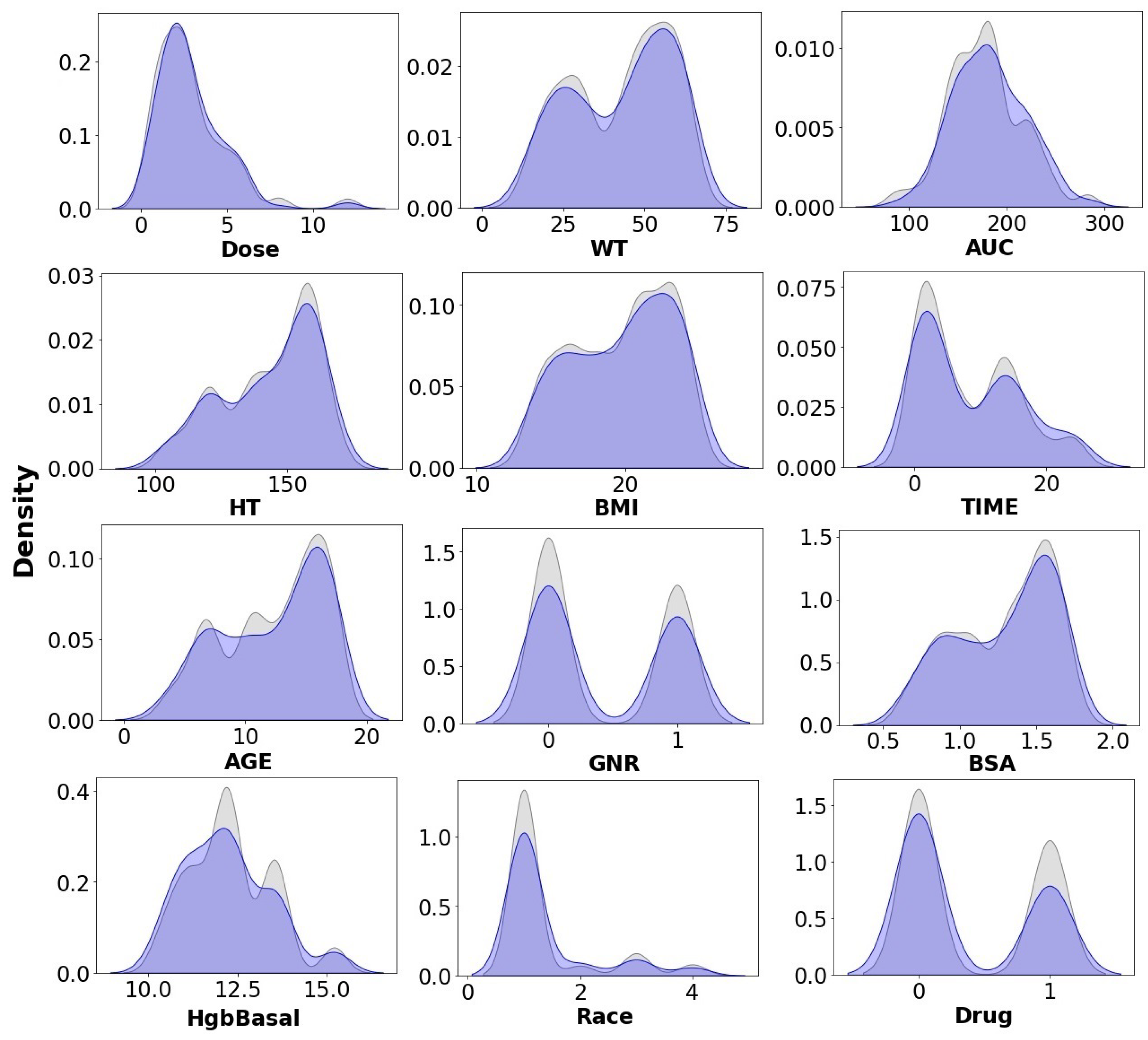
A kernel density estimate (KDE) plot was developed for each variable to visualize the distribution of observations in the derivation and validation datasets. KDE represents the data using a continuous probability density curve in one or more dimensions. This method was taken into account to ensure the cohorts were comparable [27]. In order to assess if there were significant differences between the derivation and validation cohorts, the propensity score matching method [28] was applied.

2.2. Validation Methods

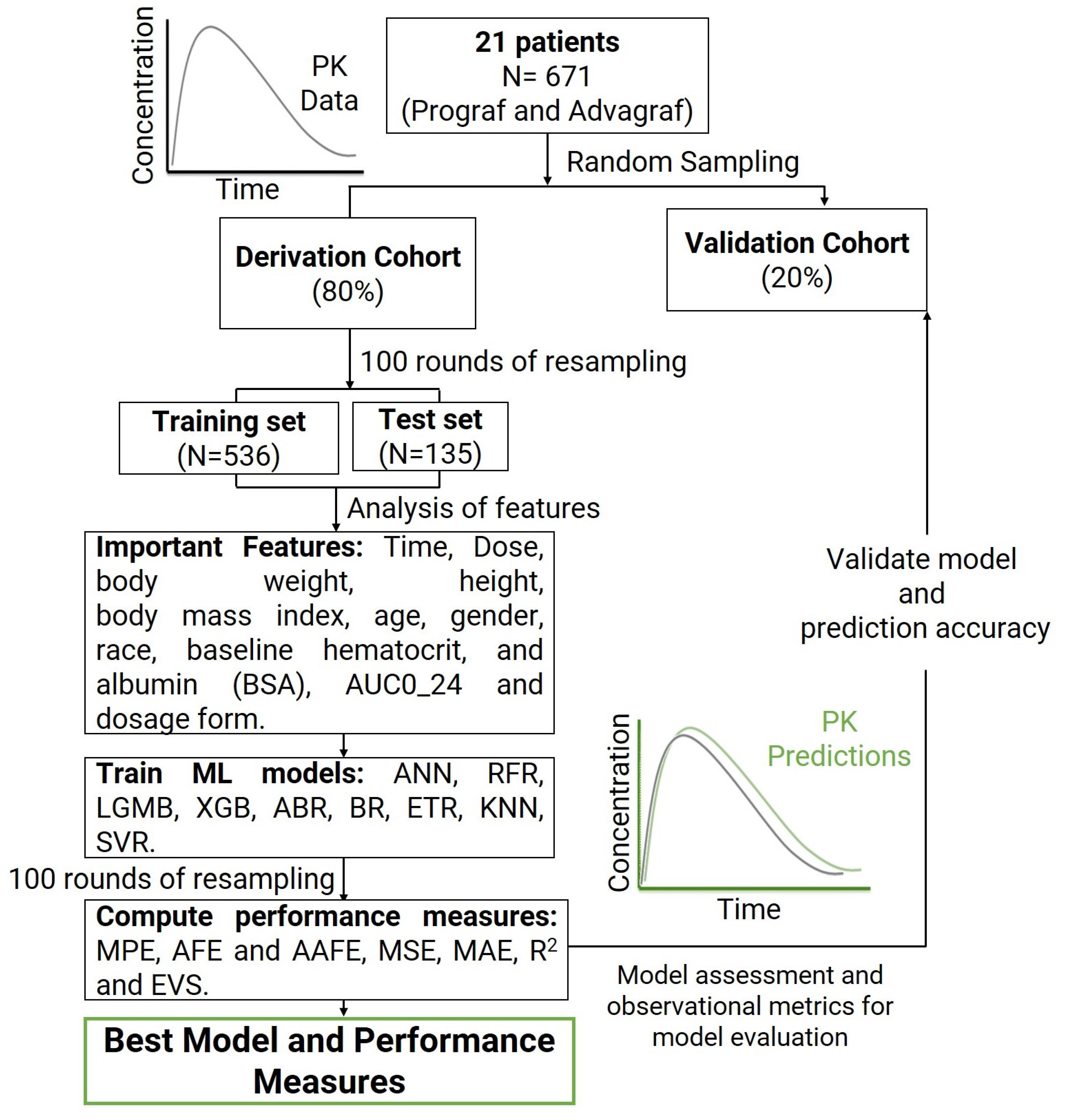
Figure 1 shows the research flow chart, which is described next. To divide the eligible patients into training and validation cohorts, a random selection was performed, where $80\%$ of the patients constituted the ‘derivation cohort’ for developing the dose-prediction algorithm. The remaining $20\%$ of patients formed the ‘validation cohort’ for testing and predicting plasma concentrations over time.

To evaluate the information required by ML algorithms for accurate predictions, different scenarios were considered, including varying numbers of observed TAC concentrations as input variables, in addition to the weighted features incorporated in the model. By conducting these analyses, we aimed to better understand how much data are needed for ML models to make reliable predictions and optimize the use of available clinical PK data in drug development.

The prediction performance of the model and observational metrics for model evaluation were developed for patients whose predicted dose fell within $20\%$ of the actual dose in the validation cohort. Additionally, 100 rounds of resampling were executed to minimize overfitting and ensure reliable results using the pandas.DataFrame.resample method [29]. A fixed seed for the pseudorandom generator was used to ensure that results are reproducible across all machine learning methods.

2.3. Models

ML is a branch of statistical research that focuses on training computational algorithms to process, classify, and manipulate datasets. ML techniques are typically categorized into supervised, unsupervised, and semisupervised learning methods [30]. Nine advanced ML models were fitted and evaluated: artificial neural networks (ANN) [31], random forest regressor (RFR) [32], LGBM regressor (LGMB), XGB regressor (XGB) [33], AdaBoost regressor (ABR) [34], bagging regressor (BR) [35], extra-trees regressor (ETR) [36], K neighbors regressor (KNN) [37], and support vector regression (SVR) [38].

As ML models have important parameters that cannot be directly estimated from the data, tuning parameters allow the adjustment of settings within an algorithm to optimize performance. These parameters are referred to as tuning parameters because there is no analytical formula available to calculate an appropriate value. For this reason, ML models were optimized by testing different model parameters through hyperparameter tuning (

Table 1. Hyperparameters for models.

Model	Core Hyperparameters
ANN	epoch_nr = 5, batch_size = 64, dense = 256, optimizer = sgd, metrics = accuracy, binary_accuracy, activation = relu
RFR	n_estimators = 1000, n_jobs = −1, random_state = 1, min_samples_split = 2, max_features = 10, min_samples_leaf = 1, max_depth = 16
LGMB	n_estimator = 1000 s, learning_rate = 0.1
XGB	n_estimators = 1000, subsample = 0.7
ABR	learning_rate = 0.1, max_depth = 16, subsample = 0.7, n_estimators = 1000, gamma = 0.0003
BR	n_estimators = 1000
ETR	none
KNN	radius = 1.0, weights = uniform, algorithm = auto, leaf_size = 100, p = 2, metric = minkowski, metric_params = None, n_jobs = None
SVR	C = 20, epsilon = 0.008, gamma = 0.0003

).

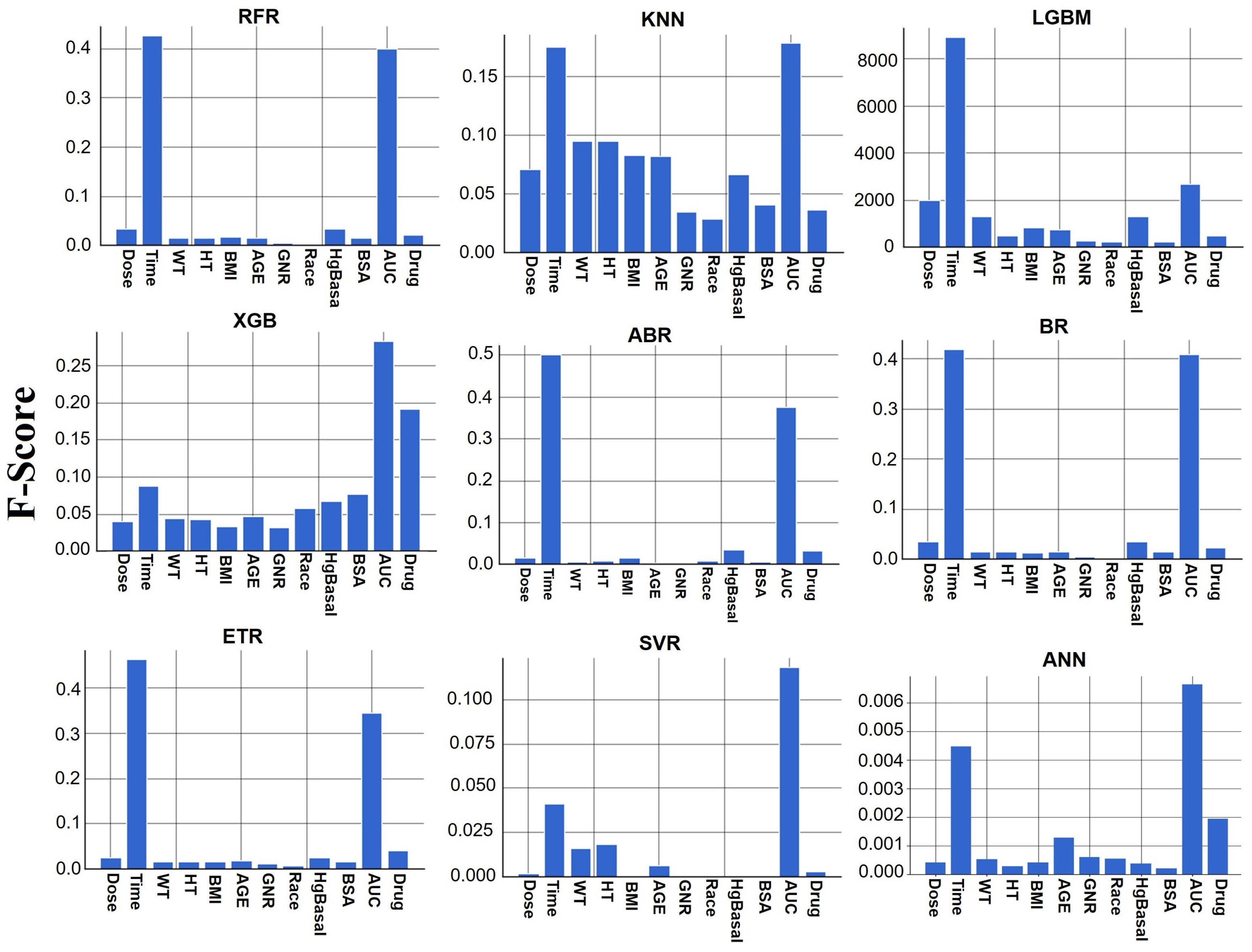
During the training phase, the best ML model assesses each feature and assigns it a weight, which determines how strongly the feature contributes to the prediction of the target variable. The goal is to explain the prediction of a target variable Y by quantifying the contribution of each feature to that prediction. The F-score values indicate how the prediction should be fairly distributed among the features [39].

2.4. Performance Metrics

The prediction performance of ML models were calculated using the percentage prediction error (PE) as shown in Equation (1), and mean percentage prediction error (MPE), as displayed in Equation (2), where PRED_i refers to the predicted value for individual i in the sample set I, with $\left|I\right|=n$, and OBS_i is the observed value for i:

$$PE(\%)=\frac{PRE{D}_i-OB{S}_i}{OB{S}_i}·100$$

(1)

$$MPE=\frac{1}{n}·\sum _{i\in I}^{}PE$$

(2)

The overall predictability of the model is evaluated in terms of bias and precision using the conventional metrics of average-fold error (AFE), as shown in Equation (3), and absolute average-fold error (AAFE), as displayed in Equation (4):

$$AFE={10}^{\frac{1}{n}{\sum }_{}log\frac{PRE{D}_i}{OB{S}_i}}$$

(3)

$$AAFE={10}^{\frac{1}{n}{\sum }_{}\left|log\frac{PRE{D}_i}{OB{S}_i}\right|}$$

(4)

If the AFE and AAFE values are between 0.8- and 1.25-fold, then the predictive performance of the model is considered to be reasonably satisfactory [40,41]. In addition to the aforementioned metrics, the following traditional ones were implemented as well: mean squared error (MSE) as displayed in Equation (5), mean absolute error (MAE) as shown in Equation (6), R² score as shown in Equation (7), and explained variance score (EVS) as displayed in Equation (8) [42]. MSE and MAE are risk metrics representing the expected value of squared (quadratic) error or loss. A lower score, closer to $0.0$, indicates better performance. R² represents the proportion of variability in the target variable Y explained by the model’s independent variables. A high R² implies a strong fit, indicating how well the model predicts hypothetical samples. The best achievable score is $1.0$. EVS calculates the explained variance regression score. Higher values, closer to $1.0$, indicate better performance.

$$\mathrm{MSE}=\frac{{\sum }_{i\in I}{(OB{S}_i-PRE{D}_i)}^2}{n}$$

(5)

$$\mathrm{MAE}=\frac{{\sum }_{i\in I}|OB{S}_i-PRE{D}_i|}{n}$$

(6)

$$R^2=\sqrt{\frac{{\sum }_{i\in I}{(OB{S}_i-PRE{D}_i)}^2}{n}}$$

(7)

$$EVS=1-\frac{Var\{OBS-PRED\}}{Var\left\{OBS\right\}}$$

(8)

2.5. External Evaluation

External evaluation of ML models involves using an independent dataset to assess the accuracy and bias of the overall model performance in subjects with characteristics similar to those with whom the models were developed. It is also a useful methodology to evaluate and select the most accurate and precise model for a different target population. Therefore, external evaluation is an appropriate approach for selecting ML models available for model-informed precision dosing.

The external predictability of ML models was evaluated using the pediatric renal transplantation dataset from the following references: (i) the pharmacokinetics, efficacy, and safety of once-daily tacrolimus formulation (Prograf and Advagraf) were assessed in 34 stable pediatric kidney transplant recipients [43]; (ii) the bioavailability of Prograf and Advagraf was evaluated in 21 stable renal transplant pediatric patients for determining serial blood samples of tacrolimus [44]; and (iii) a Phase II study comparing the pharmacokinetics of tacrolimus in stable pediatric kidney, liver, or heart transplant patients [45]. Data from these references were extracted using the Plot Digitizer software (Version v3) [46]. This is a free data-extraction program that invokes the external tool AutoTrace for automatic curve detection.

2.6. Software

All analyses in this study were performed using Python, a cross-platform, free, and open-source programming environment. Python was utilized for dataset manipulation, data visualization, and ML model training. Specifically, the Python programming language version 3.9.7 was utilized, along with its powerful packages for data management, statistical computing, and graphical production capabilities. Default parameters were used for each programming function unless otherwise specified.

For regression modeling and algorithm implementation, the sklearn package (version 1.3.0) was utilized. The ensemble package was used to fit the RFR, BR, ETR, and ABR models. The regression package was used for the KNNR model, the neural network package for the NN model, the SVM package for the SVR model, and the Xgboost and Lightgbm packages for XGB and LGMB, respectively [47]. Similarly, the SciPy package (version 1.11.1) [48] was employed to implement statistical tests. Finally, the Seaborn package (version 0.12.2) [49] was used to plot heat map figures and analyze the feature importance of each ML method.

3. Results

This section shows the results obtained, covering basic patient characteristics, model performance, feature analysis, predictions, external validation, and clinical significance.

3.1. Basic Patient Characteristics

The basic characteristics of the 21 renal transplant pediatric patients are shown in

Table 2. Basic characteristic of the patients.

Variable	The Derivation Cohort (N = 536)	The Validating Cohort (N = 135)	p Value *
Continuous variable mean (sd)
Tacrolimus stable dose (mg/day)	1.99 (1.21)	2.29 (1.37)	0.95
Age (year)	12.14 (4.07)	12.85 (4.11)	0.98
Weight (cm)	41.96 (15.17)	44.79 (15.39)	0.8
Height (cm)	142.88 (17.76)	145.27 (17.63)	0.92
BMI (kg/m2)	19.58 (3.29)	20.29 (3.31)	0.78
Hemoglobin (g/dL)	12.26 (1.13)	12.36 (1.37)	0.46
BSA (m2)	1.28 (0.31)	1.33 (0.32)	0.85
AUC (ng/mLh)	180.1(33.26)	185.42 (32.45)	0.17
Categorical variable (%)
Sex	Male (57) and Female (43)	Male (57) and Female (43)	0.84
Race	White (81), Black (10), Asian (5) and Other (5)	White (79), Black (10), Asian (6) and Other (5)	0.95
Dosage form	Prograf (64) and Advagraf (36)	Prograf (58) and Advagraf (42)	0.17

* Computed using the t-test for continuous variables and the chi-squared test for categorical variables.

. Continuous variables are presented as mean ± standard deviation, along with the corresponding p-value obtained from the t-test. Categorical variables are displayed as percentages, accompanied by the associated p-value derived from the chi-squared test. There were no significant differences in demographic information, clinical, and PK data between the derivation cohort ($N=536$) and the validation cohort ($N=135$).

For example, the mean tacrolimus stable dose among these patients was $1.99\pm 1.21$ mg/day and $2.29\pm 1.37$ mg/day, respectively. Patients in the derivation cohort were an average age of $12.28\pm 4.08$ years old, and $57\%$ were males. Similarly, patients in the validation cohort were $12.85\pm 4.11$ years old, and, again, $57\%$ were males.

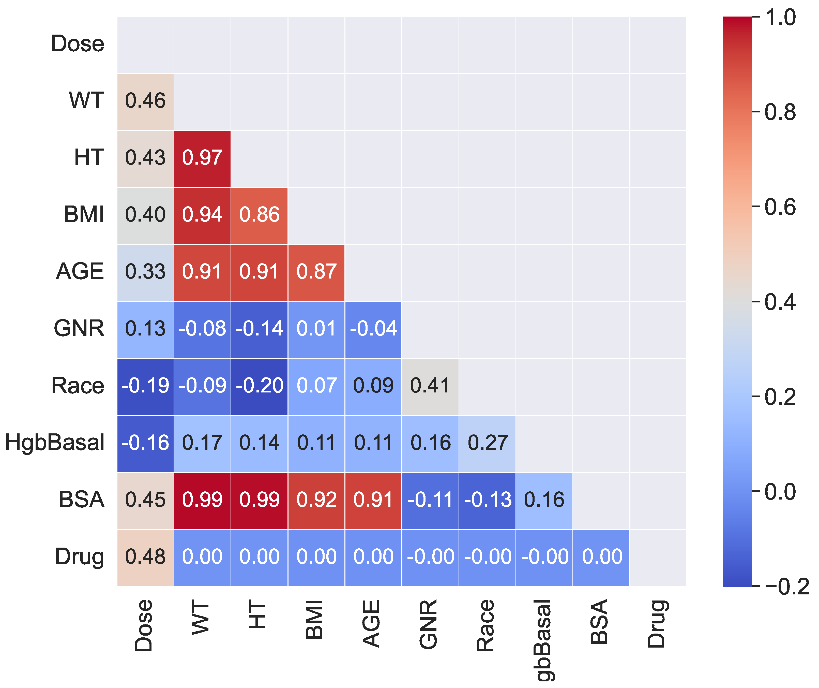
Figure 2 displays a heat map plot showing the correlation coefficients among WT, HT, BMI, AGE, GNR, Race, HgbBasal, BSA, and drug. Since BMI and BSA depend on WT and HT, there are positive correlations between these variables. Additionally, AGE is positively correlated with both WT and HT. The remaining correlation coefficients approach zero, indicating that there are no more statistically significant correlations.

Figure 3 displays KDE plots for all variables used in the models, showing the distribution of observations in the derivation and validation dataset. These plots suggest that there are no significant differences between the derivation and validation cohorts. Thus, they are considered comparable. Figure 4 shows the propensity score matching plot for the derivation and validation cohorts. There is a complete overlap between both groups. We concluded that the cohorts are comparable and can be used for training models.

3.2. Model Performance

A comprehensive comparison of models based on the derivation cohort is presented in

Table 3. Performance of the models.

Metrics Model	ANN	RFR	LGMB	XGB	ABR	BR	ETR	KNN	SVR
MPE	−0.404	−0.378	−0.703	−0.886	−0.097	−0.605	−0.161	1.214	−0.394
AFE	0.987	0.992	0.989	0.986	0.991	0.999	0.995	1.002	0.987
AAFE	1.125	1.070	1.071	1.077	1.107	1.071	1.063	1.114	1.109
MSE	0.1	0.03	0.043	0.048	0.074	0.04	0.035	0.089	0.087
MAE	0.255	0.132	0.145	0.156	0.217	0.145	0.132	0.233	0.225
R2	0.41	0.8	0.74	0.71	0.56	0.77	0.8	0.89	0.48
EVS	0.43	0.8	0.74	0.71	0.56	0.77	0.8	0.72	0.49

. Among the various models considered, namely, KNN, BR, RFR, and ETR, consistent results were observed in terms of the R² value ($89\%$, $77\%$, $80\%$, and $80\%$, respectively) and MPE ($1.214$, $-0.605$, $-0.378$, and $-0.161$, respectively). Furthermore, LGBM and XGB models exhibited promising outcomes, similar to other machine learning analyses, for TAC blood concentrations in adults [8]. Variables such as membrane permeability, plasma protein binding, and total body water play pivotal roles in explaining alterations in medication distribution between pediatric and adult populations. Notably, significant differences in drug metabolism were identified between these two groups, highlighting variations in different metabolic enzymes. The variance stems from the immaturity of glomerular filtration, renal tubular secretion, and tubular reabsorption at birth, alongside their subsequent maturation, thereby contributing to the divergence in drug excretion patterns between children and adults. Thus, the intricacies of pharmacokinetics and pharmacodynamics in the pediatric and adult cohorts are multifaceted [50]. This study was specifically centered on a pediatric TAC dataset. Despite the intrinsic disparities in pharmacokinetics and pharmacodynamics between pediatric and adult subjects, the overall outcomes of the investigation underscored the competence of machine learning methods in accurately predicting TAC concentration–time profiles in the pediatric demographic. Within this context, the ExtraTreesRegressor (ETR) algorithm emerged as the top performer among all models for forecasting TAC blood concentrations in the pediatric population. In comparison to KNN, BR, and RFR models, the ETR algorithm exhibited superior performance, particularly evident in terms of AFE and AAFE. ETR demonstrated an AAFE value of $1.063$, which is the closest approximation to unity among all the machine learning methods scrutinized in this study.

Figure 5 allowed us to perform a visual evaluation of the regression models. The performance metrics of the models displayed in Table 3 are consistent with the patterns observed in the scatter plots. Specifically, the ETR, BR, RFR, XGB, KNN, and LightGBM models exhibit an excellent regression fit, with data points closely aligned to the diagonal line, which represents the actual values. Deviations from this line reveal the model’s error. However, the scatter plot alone does not provide actionable insights on how to improve the model. To gain further insights, residual plots (Figure 6) were examined to analyze whether the residuals follow a homoscedastic (i.e., equal variance) or heteroscedastic distribution. Unequal variance in residuals causes heteroscedastic dispersion and may be represented by different shapes. The ETR, BR, RFR, XGB, KNN, and LGBM models show uncorrelated residuals, with almost zero expected values and constant variance, indicating homoscedasticity. In addition, other ML models, such as ANN, display heteroscedastic structures, suggesting varying variance in prediction errors.

The scatter plot and residual plots helped us evaluate the performance of regression models. The selected ETR algorithm, along with BR, RFR, XGB, and LGMB, demonstrate excellent predictive capabilities with minimal residuals, while models with heteroscedastic structures, like ANN, may require further improvements.

3.3. Feature Analysis

The features’ relevance for each model is shown in Figure 7. AUC and time have a significant effect on the blood concentration of TAC. Additionally, in the ANN and XGB models, drug formulation is identified as an important feature. On the contrary, the remaining variables such as weight, age, height, gender, sex, and race have relatively minor importance.

3.4. Predictions of Tacrolimus Plasma Concentration over Time

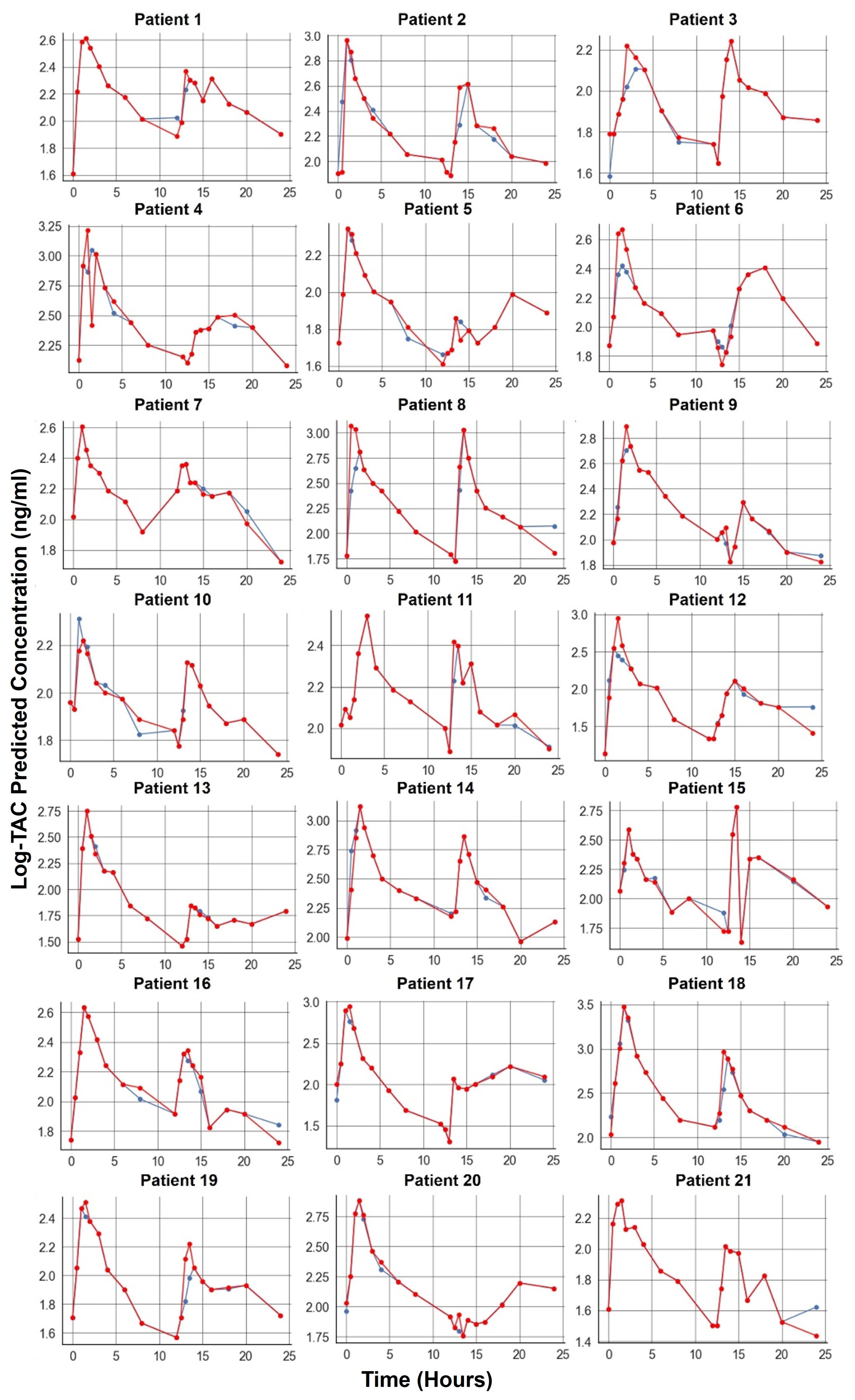
The analysis of the ETR model after Prograf and Advagraf administration for the data of 21 pediatric patients is shown in Figure 8 and Figure 9. The concentration–time profiles of the children are observed to be quite heterogeneous, characterized by a distribution phase with a remarkable half-life, followed by an elimination phase with a long half-life. This PK profile aligns with the typical behavior of tacrolimus when administered as Prograf and Advagraf formulations [43,44,45]. The ETR model demonstrates a wide ability to accurately account for and predict these standard PK profiles associated with tacrolimus oral administration. Thus, ML models, particularly the ETR model, hold promise for effectively predicting human plasma concentration–time profiles of tacrolimus. The findings from this analysis contribute to the growing evidence supporting the potential of ML in pharmacokinetics and its application in predicting drug behaviors in pediatric populations.

3.5. External Validation

The external validation serves to assess the performance of the ETR model in predicting TAC concentration–time profiles in pediatric patients, using data from published studies. Observed longitudinal PK profiles following single TAC administration of Prograf and Advagraf in pediatric renal transplant patients were obtained from published PK studies in stable pediatric clinical cases found in the literature [43,44,45]. The mean baseline demographic and characteristic values of the patients from these external references are presented in

Table 4. Mean patient baseline demographics and characteristic values from external references.

Reference	Carcas-Sansuán et al. [44]		Min et al. [43]		Rubik et al. [45]
Variable	Prograf	Advagraf	Prograf	Advagraf	Prograf	Advagraf
Continuous variable mean (sd)
Tacrolimus stable dose (mg/day)	2.4	4.8	1.845	3.69	3.81	7.62
Age (year)	12.29	12.29	12.3	12.3	10.8	10.8
Weight (cm)	42.85	42.85	40.7	40.7	38.7	38.7
Height (cm)	143.4	143.4	143.7	143.7	138.1	138.1
BMI (kg/m2)	20.8	20.8	19	19	20.29	20.29
Hemoglobin (/dL)	12 *	12 *	12 *	12 *	12 *	12 *
BSA (m2)	1.44	1.44	1.27	1.27	1.2	1.2
AUC (ng/mLh)	206.6	200.7	147.6	144.73	175.4	169.5

* Data not reported in references. Mean value for pediatric 6–18 years [51].

. These data were used as inputs for predictions using the ETR model.

In order to characterize the longitudinal PK behavior of TAC concentration–time in pediatric patients, the ETR model was applied to predict concentrations. The ETR model was defined as the best option based on the metrics identified in Table 3. The resulting predictions are depicted in Figure 10.

The metrics of the ETR model for exposure PK concentration–time samples from the selected references are displayed in

Table 5. Performance of validation with ETR model.

Reference	Carcas-Sansuán et al. [44]		Min et al. [43]		Rubik et al. [45]
Metrics Model	Prograf	Advagraf	Prograf	Advagraf	Prograf	Advagraf
MPE	−4.32	−7.387	−5.72	0.68	−12.519	−2.01
AFE	1.05	1.086	1.142	1.12	1.155	1.067
AAFE	1.082	1.109	1.072	1.007	1.15	1.023
MSE	0.851	1.567	1.193	1.07	1.439	0.24
MAE	0.691	0.918	0.845	0.687	1.01	0.44
R2	0.86	0.68	0.83	0.79	0.67	0.94
EVS	0.88	0.79	0.83	0.79	0.88	0.94

. The values demonstrate a successful characterization of the observed data. For instance, the AFE and AAFE values between $0.8$ and $1.25$ indicate that the ETR model’s predictions are close to the observed data. This level of accuracy suggests that the ETR model is robust and reliable for predicting TAC pharmacokinetics in pediatric patients across different populations and clinical scenarios.

The successful external validation of the ETR model further supports its suitability for application in real-world clinical settings, providing clinicians with valuable tools for optimizing individualized treatment strategies and improving therapeutic outcomes in pediatric patients receiving TAC.

3.6. Clinical Significance

The comparison between the model predictions and the observed values throughout the research demonstrates a consistently good predictive performance of the ETR model. To assess the clinical significance of the dosing algorithm, the researchers calculated the percentage of samples from patients for whom the actual concentration–time sample of TAC was successfully predicted. They considered different percentages to illustrate how well the predictions aligned with the observed data.

Table 6. Successful ETR model TAC predictions.

Reference	Carcas-Sansuán et al. [44]		Min et al. [43]		Rubik et al. [45]
% *	Prograf	Advagraf	Prograf	Advagraf	Prograf	Advagraf
10%	61.14%	69.23%	46.15%	76.92%	53.85%	92.31%
15%	76.92%	69.23%	69.23%	84.62%	61.54%	100%
20%	92.3%	84.62%	76.92%	84.62%	76.92%	100%

* Success rates at different percentages.

presents the results for the success rates at different percentages, specifically $10\%$, $15\%$, and $20\%$. The percentages in the table indicate the proportion of samples for which the ETR model’s predictions are accurate within the specified range of the actual concentration–time data.

The model’s ability to achieve a high success rate across multiple percentage thresholds further validates its effectiveness in providing clinically relevant and accurate predictions.

4. Discussion

Our study’s findings indicate that most of the ML models used for TAC prediction demonstrated a high accuracy. The models that achieved better results for AFE and AAFE values were the ETR, BR, RFR, KNN, XGB, and LGMB models.

The ETR model, which implements a meta-estimator involving randomized decision trees and averaging, achieved slightly better performance. This advantage could be attributed to its ability to control overfitting and improve predictive accuracy by using multiple subsamples of the dataset. This finding emphasizes the importance of considering the characteristics of different ML models and their potential advantages in specific scenarios.

The top three ML models for TAC concentration prediction in this study were ETR, BR, and RFR, while XGB and LGMB also demonstrated good accuracy. This is similar to the findings of other research on TAC predictions in adults [8,33].

The results show that there were no significant accuracy differences between the top three or five best models, which suggests that these models perform comparably well.

Overall, the successful performance of ML models in predicting TAC concentrations in pediatric patients suggests that they could be valuable tools in real-world clinical settings. By providing accurate predictions of TAC concentrations, these models can aid in individualized treatment strategies, optimizing dosage regimens, and ultimately improving therapeutic outcomes for pediatric renal transplant recipients.

The feature importance analysis for the ETR model revealed that the area under the concentration–time curve (AUC) of TAC blood concentration had a significant effect on TAC blood concentration. This finding aligns with the existing knowledge in the field, as AUC is a critical PK parameter used to assess drug exposure and is considered the preferred measure for TAC exposure in clinical practice [52,53]. Interestingly, the importance of AUC was also supported by other ML models used in this study, including RFR, LGMB, ABR, and BR. This consistency in feature importance across different models reinforces the significance of AUC as a critical factor in predicting TAC blood concentrations and its relevance in guiding individualized dosing strategies. Furthermore, some of the models considered the importance of the pharmaceutical form of TAC (Prograf vs. Advagraf) in predicting blood concentrations. This is a logical consideration, as the dosing regimens and concentration–time profiles differ between Prograf (twice-daily administration) and Advagraf (once-daily administration). The number of maximum concentration points for each pharmaceutical form is indeed different, which could influence the overall concentration–time profile. Therefore, taking into account the pharmaceutical form as a feature in the models can help capture these differences and improve prediction accuracy.

Validating ML methods for TAC predictions in the presence of other co-administered drugs is crucial for real-world clinical applications. The PK of TAC can be affected by drug–drug interactions, where the presence of other drugs in the patient’s regimen can influence its metabolism, absorption, distribution, and elimination.

In addition, drug interactions may not only affect the PK of TAC but also impact the therapeutic outcomes and safety of the patient. Therefore, the ability of ML models to accurately predict TAC blood concentrations in the presence of co-administered drugs can have significant clinical implications, guiding clinicians in optimizing dosing regimens and minimizing the risk of adverse drug events [54].

Unfortunately, this dataset does not take into account genomic information. Despite numerous factors that may affect the pharmacokinetics of tacrolimus, genetic factors are quite important and common. TAC is metabolized by two enzymes of the cytochrome P450 family: CYP3A5 and CYP3A4. The effect of CYP3A5 and CYP3A4 genotypes on TAC bioavailability has been demonstrated, and a significant portion of the interindividual variability in its PK is explained by mutations in the CYP3A4 and CYP3A5 enzymes. For example, studies have shown that the mean dose-adjusted blood TAC concentration was significantly higher among CYP3A53 homozygotes compared to carriers of the wild-type allele (CYP3A51) [55]. In a recent prospective study, a group of kidney transplant patients received a TAC dose either based on the CYP3A5 genotype (the adapted group) or according to the standard regimen (the control group) [56]. Consequently, additional studies are necessary to determine whether the pharmacogenetic approach could help reduce the necessity for induction therapy and co-immunosuppressors [55].

ML methods have become a prominent trend in predicting drug concentrations in the blood, and this approach has also been applied to predict TAC blood concentrations in previous research. The majority of these studies utilized artificial neural networks and regression models for their predictions [8,11,57,58,59,60,61].

However, it is essential to acknowledge that these earlier studies faced certain limitations. Firstly, they often dealt with a relatively limited amount of data, which may impact the generalizability of their models. Additionally, the lack of external validation in many of these studies raises concerns about the robustness and reliability of their findings.

Furthermore, when comparing modeling approaches in PK, there are some key points to consider. PK methods primarily focus on estimating parameters for the structural model, variability, and covariate model parameters within a population, which contributes to mechanistic understanding, biological interpretability of the results, and the ability to simulate in silico experiments from the model. Conversely, ML is primarily geared towards predicting outcomes and ML has the inherent danger of producing results that are not therapeutically meaningful. Consequently, PK/PD analysis provides valuable mechanistic insights into biological processes, whereas ML models, while trained more swiftly, offer fewer mechanistic insights and can be perceived as enigmatic ’black boxes’, making it challenging to extract underlying mechanisms [6]. This underscores the necessity for ML to have access to substantial training data that can reasonably be assumed to be exchangeable with the test data. Conversely, Bayesian inference excels when dealing with sparse data and a dense model, thereby requiring fewer patients to obtain meaningful results in PK methods [7].

Because of the numerous issues that PM and ML encounter, research in this field remains in its exploratory phase, underscoring the need for further investigation and validation. The fusion of PK and ML holds the potential to yield precise estimations of drug exposure by simulating rich concentration-versus-time profiles, by exploring and learning the relationships within all the patient covariates [62] or by using faster models and performing faster analyses [63]. For instance, the ML approach has been shown to confer advantages over traditional approaches, including increased accuracy and reduced variance [64]. These innovative approaches represent a significant advancement compared to the prior situation where extensive databases were essential to train an ML algorithm, leaving scarce independent datasets for validation purposes [7].

As ML methods continue to advance and more data become available, it is hoped that these limitations can be addressed and the potential of ML fully harnessed in drug concentration prediction, benefiting both adult and pediatric populations alike.

5. Conclusions

The therapeutic drug monitoring approach has been widely applied in clinical practice to assess specific medications at predetermined intervals. This technique ensures a consistent drug concentration in a patient’s bloodstream, thereby improving the tailoring of individual dosage plans. Concurrently, pharmacokinetics models have been extensively utilized to establish the link between drug exposure and its resulting effects, as demonstrated by metrics like the area under the curve. Nonetheless, innovative and successful predictive methods from diverse fields have emerged as viable alternatives to conventional PK predictions.

In this study, a machine learning model was established to categorize blood tacrolimus concentration in pediatric patients who had undergone kidney transplants. While clinical data present certain limitations such as data dependency and bias, resampling techniques were employed to address these issues. Variables were also screened based on their importance, and the performance of nine different models was compared. The primary influencing factor on blood TAC concentration was determined to be the AUC variable. Ultimately, the extra-trees regression model was chosen as the best predictive model with an R2 value of 80% and an MPE of −0.161, although other models performed nearly as well, indicating strong prediction capabilities across all of them. It should also be highlighted that most models exhibited satisfactory predictions, meeting the criteria of AFE and AAFE falling between 0.8- and 1.25-fold with 0.999 and 1.063, respectively, for internal validation. The external validations developed with the extra-trees regression model were also successful under the criteria of AFE and AAFE, falling between 0.8- and 1.25-fold. On the other hand, the extra-trees regression model presents the results for the success rates at different percentages, where specifically $15\%$ and $20\%$ are accurate within the specified ranges of 60–85% and 75–100%, respectively, of the actual external validation concentration–time data.

Hence, this study offers valuable insights into the predictive capacity of machine learning for TAC blood concentration in children, which is similar to other machine learning analyses conducted for TAC blood concentrations in adults. Despite allometric and PK/PD differences between adults and children, machine learning methods accurately projected TAC concentration–time patterns for pediatrics, akin to the achievements seen in adult studies. In addition, essential genetic factors are quite important to take into account the effect of CYP3A5 and CYP3A4 genotypes on TAC bioavailability, which has been demonstrated, and a significant portion of the interindividual variability in its PK is explained by mutations in the CYP3A4 and CYP3A5 enzymes. Nevertheless, further extensive research is necessary to address potential bias and to further validate and refine these predictive models to achieve a high success rate effectiveness in providing clinically relevant and accurate predictions.

As a result, this study delved into the ability of machine learning to predict two pharmaceutical forms of TAC blood concentration and validated these predictions against independent references for pediatric kidney transplant cases. The study’s findings indeed highlight the predictive potential of machine learning to a certain extent. As a future research line, new studies could analyze the influence of pharmacogenomics, an aspect not addressed in this study due to data limitations.

References

1. Stone, J.A.; Banfield, C.; Pfister, M.; Tannenbaum, S.; Allerheiligen, S.; Wetherington, J.D.; Krishna, R.; Grasela, D.M. Model-based drug development survey finds pharmacometrics impacting decision making in the pharmaceutical industry. J. Clin. Pharmacol. 2010, 50, 20S–30S. [Google Scholar] [CrossRef] [PubMed]
2. Wang, Y.; Zhu, H.; Madabushi, R.; Liu, Q.; Huang, S.M.; Zineh, I. Model-informed drug development: Current US regulatory practice and future considerations. Clin. Pharmacol. Ther. 2019, 105, 899–911. [Google Scholar] [CrossRef] [PubMed]
3. Mao, J.; Chen, Y.; Xu, L.; Chen, W.; Chen, B.; Fang, Z.; Qin, W.; Zhong, M. Applying machine learning to the pharmacokinetic modeling of cyclosporine in adult renal transplant recipients: A multi-method comparison. Front. Pharmacol. 2022, 13, 1016399. [Google Scholar] [CrossRef] [PubMed]
4. Koch, G.; Pfister, M.; Daunhawer, I.; Wilbaux, M.; Wellmann, S.; Vogt, J.E. Pharmacometrics and machine learning partner to advance clinical data analysis. Clin. Pharmacol. Ther. 2020, 107, 926–933. [Google Scholar] [CrossRef] [PubMed]
5. Danishuddin; Kumar, V.; Faheem, M.; Lee, K.W. A decade of machine learning-based predictive models for human pharmacokinetics: Advances and challenges. Drug Discov. Today 2022, 27, 529–537. [Google Scholar] [CrossRef]
6. McComb, M.; Bies, R.; Ramanathan, M. Machine learning in pharmacometrics: Opportunities and challenges. Br. J. Clin. Pharmacol. 2022, 88, 1482–1499. [Google Scholar] [CrossRef]
7. Keutzer, L.; You, H.; Farnoud, A.; Nyberg, J.; Wicha, S.G.; Maher-Edwards, G.; Vlasakakis, G.; Moghaddam, G.K.; Svensson, E.M.; Menden, M.P.; et al. Machine learning and pharmacometrics for prediction of pharmacokinetic data: Differences, similarities and challenges illustrated with rifampicin. Pharmaceutics 2022, 14, 1530. [Google Scholar] [CrossRef]
8. Yuan, W.; Sui, L.; Xin, H.; Liu, M.; Shi, H. Discussion on machine learning technology to predict tacrolimus blood concentration in patients with nephrotic syndrome and membranous nephropathy in real-world settings. BMC Med. Inform. Decis. Mak. 2022, 22, 336. [Google Scholar] [CrossRef]
9. Lu, J.; Bender, B.; Jin, J.Y.; Guan, Y. Deep learning prediction of patient response time course from early data via neural-pharmacokinetic/pharmacodynamic modelling. Nat. Mach. Intell. 2021, 3, 696–704. [Google Scholar] [CrossRef]
10. Tang, B.H.; Guan, Z.; Allegaert, K.; Wu, Y.E.; Manolis, E.; Leroux, S.; Yao, B.F.; Shi, H.Y.; Li, X.; Huang, X.; et al. Drug clearance in neonates: A combination of population pharmacokinetic modelling and machine learning approaches to improve individual prediction. Clin. Pharmacokinet. 2021, 60, 1435–1448. [Google Scholar] [CrossRef]
11. Woillard, J.B.; Labriffe, M.; Debord, J.; Marquet, P. Tacrolimus exposure prediction using machine learning. Clin. Pharmacol. Ther. 2021, 110, 361–369. [Google Scholar] [CrossRef] [PubMed]
12. Woillard, J.B.; Labriffe, M.; Debord, J.; Marquet, P. Mycophenolic acid exposure prediction using machine learning. Clin. Pharmacol. Ther. 2021, 110, 370–379. [Google Scholar] [CrossRef] [PubMed]
13. Dara, S.; Dhamercherla, S.; Jadav, S.S.; Babu, C.M.; Ahsan, M.J. Machine learning in drug discovery: A review. Artif. Intell. Rev. 2022, 55, 1947–1999. [Google Scholar] [CrossRef] [PubMed]
14. Vora, L.K.; Gholap, A.D.; Jetha, K.; Thakur, R.R.S.; Solanki, H.K.; Chavda, V.P. Artificial Intelligence in Pharmaceutical Technology and Drug Delivery Design. Pharmaceutics 2023, 15, 1916. [Google Scholar] [CrossRef]
15. Rai, A. Explainable AI: From black box to glass box. J. Acad. Mark. Sci. 2020, 48, 137–141. [Google Scholar] [CrossRef]
16. Thervet, E.; Loriot, M.; Barbier, S.; Buchler, M.; Ficheux, M.; Choukroun, G.; Toupance, O.; Touchard, G.; Alberti, C.; Le Pogamp, P.; et al. Optimization of initial tacrolimus dose using pharmacogenetic testing. Clin. Pharmacol. Ther. 2010, 87, 721–726. [Google Scholar] [CrossRef]
17. Budde, K.; Bunnapradist, S.; Grinyo, J.; Ciechanowski, K.; Denny, J.; Silva, H.; Rostaing, L.; Envarsus Study Group. Novel once-daily extended-release tacrolimus (LCPT) versus twice-daily tacrolimus in de novo kidney transplants: One-year results of Phase III, double-blind, randomized trial. Am. J. Transplant. 2014, 14, 2796–2806. [Google Scholar] [CrossRef]
18. Shuker, N.; Bouamar, R.; van Schaik, R.H.; Clahsen-van Groningen, M.C.; Damman, J.; Baan, C.C.; van de Wetering, J.; Rowshani, A.T.; Weimar, W.; van Gelder, T.; et al. A randomized controlled trial comparing the efficacy of Cyp3a5 genotype-based with body-weight-based tacrolimus dosing after living donor kidney transplantation. Am. J. Transplant. 2016, 16, 2085–2096. [Google Scholar] [CrossRef]
19. Fu, Q.; Jing, Y.; Liu, G.; Jiang, X.; Liu, H.; Kong, Y.; Hou, X.; Cao, L.; Deng, P.; Xiao, P.; et al. Machine learning-based method for tacrolimus dose predictions in Chinese kidney transplant perioperative patients. J. Clin. Pharm. Ther. 2022, 47, 600–608. [Google Scholar] [CrossRef]
20. Iwasaki, K. Metabolism of tacrolimus (FK506) and recent topics in clinical pharmacokinetics. Drug Metab. Pharmacokinet. 2007, 22, 328–335. [Google Scholar] [CrossRef]
21. Mika, A.; Stepnowski, P. Current methods of the analysis of immunosuppressive agents in clinical materials: A review. J. Pharm. Biomed. Anal. 2016, 127, 207–231. [Google Scholar] [CrossRef] [PubMed]
22. Andrews, L.M.; Li, Y.; De Winter, B.C.; Shi, Y.Y.; Baan, C.C.; Van Gelder, T.; Hesselink, D.A. Pharmacokinetic considerations related to therapeutic drug monitoring of tacrolimus in kidney transplant patients. Expert Opin. Drug Metab. Toxicol. 2017, 13, 1225–1236. [Google Scholar] [CrossRef] [PubMed]
23. Rahman, Z.; Zidan, A.; Khan, M.A. Tacrolimus properties and formulations: Potential impact of product quality on safety and efficacy. In Tacrolimus: Effectiveness, Safety and Drug Interactions; Nova Science Publishers Inc.: New York, NY, USA, 2013; pp. 1–39. [Google Scholar]
24. Ogden, J. The British National Formulary: Past, present and future. Prescriber 2017, 28, 20–24. [Google Scholar] [CrossRef]
25. De Gregori, S.; De Silvestri, A.; Cattadori, B.; Rapagnani, A.; Albertini, R.; Novello, E.; Concardi, M.; Arbustini, E.; Pellegrini, C. Therapeutic Drug Monitoring of Tacrolimus-Personalized Therapy in Heart Transplantation: New Strategies and Preliminary Results in Endomyocardial Biopsies. Pharmaceutics 2022, 14, 1247. [Google Scholar] [CrossRef]
26. Prado-Velasco, M.; Borobia, A.; Carcas-Sansuan, A. Predictive engines based on pharmacokinetics modelling for tacrolimus personalized dosage in paediatric renal transplant patients. Sci. Rep. 2020, 10, 7542. [Google Scholar] [CrossRef]
27. Chen, Y.C. A tutorial on kernel density estimation and recent advances. Biostat. Epidemiol. 2017, 1, 161–187. [Google Scholar] [CrossRef]
28. Benedetto, U.; Head, S.J.; Angelini, G.D.; Blackstone, E.H. Statistical primer: Propensity score matching and its alternatives. Eur. J. Cardio-Thorac. Surg. 2018, 53, 1112–1117. [Google Scholar] [CrossRef]
29. Yu, C.H. Resampling methods: Concepts, applications, and justification. Pract. Assessment, Res. Eval. 2002, 8, 19. [Google Scholar]
30. Sarker, I. Machine learning: Algorithms, real-world applications and research directions. SN Comput. Sci. 2021, 2, 160. [Google Scholar] [CrossRef]
31. Zhang, Z. A gentle introduction to artificial neural networks. Ann. Transl. Med. 2016, 4, 370. [Google Scholar] [CrossRef]
32. Speiser, J.L.; Miller, M.E.; Tooze, J.; Ip, E. A comparison of random forest variable selection methods for classification prediction modeling. Expert Syst. Appl. 2019, 134, 93–101. [Google Scholar] [CrossRef] [PubMed]
33. Zheng, P.; Yu, Z.; Li, L.; Liu, S.; Lou, Y.; Hao, X.; Yu, P.; Lei, M.; Qi, Q.; Wang, Z.; et al. Predicting blood concentration of tacrolimus in patients with autoimmune diseases using machine learning techniques based on real-world evidence. Front. Pharmacol. 2021, 12, 727245. [Google Scholar] [CrossRef] [PubMed]
34. Solomatine, D.P.; Shrestha, D.L. AdaBoost. RT: A boosting algorithm for regression problems. In Proceedings of the 2004 IEEE International Joint Conference on Neural Networks (IEEE Cat. No. 04CH37541), Budapest, Hungary, 25–29 July 2004; Volume 2, pp. 1163–1168. [Google Scholar]
35. Kadiyala, A.; Kumar, A. Applications of python to evaluate the performance of bagging methods. Environ. Prog. Sustain. Energy 2018, 37, 1555–1559. [Google Scholar] [CrossRef]
36. Takač, M.J.M.; Žuntar, I.; Takač, T. In silico prediction of the fate and toxic effects of IARC Group I anticancer drugs in the environment. Arh. Hig. Rada Toksikol. 2021, 72, 76. [Google Scholar]
37. Taunk, K.; De, S.; Verma, S.; Swetapadma, A. A brief review of nearest neighbor algorithm for learning and classification. In Proceedings of the 2019 International Conference on Intelligent Computing and Control Systems (ICCS), Madurai, India, 15–17 May 2019; pp. 1255–1260. [Google Scholar]
38. Awad, M.; Khanna, R. Support vector regression. In Efficient Learning Machines: Theories, Concepts, and Applications for Engineers and System Designers; Springer: Berlin/Heidelberg, Germany, 2015; pp. 67–80. [Google Scholar]
39. Goutte, C.; Gaussier, E. A probabilistic interpretation of precision, recall and F-score, with implication for evaluation. In Proceedings of the European Conference on Information Retrieval, Santiago de Compostela, Spain, 21–23 March 2005; Springer: Berlin/Heidelberg, Germany, 2005; pp. 345–359. [Google Scholar]
40. Puttrevu, S.K.; Arora, S.; Polak, S.; Patel, N.K. Physiologically based pharmacokinetic modeling of transdermal selegiline and its metabolites for the evaluation of disposition differences between healthy and special populations. Pharmaceutics 2020, 12, 942. [Google Scholar] [CrossRef]
41. Corral Alaejos, Á.; Zarzuelo Castañeda, A.; Jiménez Cabrera, S.; Sánchez-Guijo, F.; Otero, M.J.; Pérez-Blanco, J.S. External evaluation of population pharmacokinetic models of imatinib in adults diagnosed with chronic myeloid leukaemia. Br. J. Clin. Pharmacol. 2022, 88, 1913–1924. [Google Scholar] [CrossRef]
42. Korstanje, J. Regression. In Machine Learning on Geographical Data Using Python: Introduction into Geodata with Applications and Use Cases; Springer: Berlin/Heidelberg, Germany, 2022; pp. 251–273. [Google Scholar]
43. Min, S.I.; Ha, J.; Kang, H.; Ahn, S.; Park, T.; Park, D.; Kim, S.; Hong, H.; Min, S.; Ha, I.; et al. Conversion of twice-daily tacrolimus to once-daily tacrolimus formulation in stable pediatric kidney transplant recipients: Pharmacokinetics and efficacy. Am. J. Transplant. 2013, 13, 2191–2197. [Google Scholar] [CrossRef]
44. Carcas-Sansuán, A.J.; Espinosa-Román, L.; Almeida-Paulo, G.N.; Alonso-Melgar, A.; García-Meseguer, C.; Fernández-Camblor, C.; Medrano, N.; Ramirez, E. Conversion from Prograf to Advagraf in stable paediatric renal transplant patients and 1-year follow-up. Pediatr. Nephrol. 2014, 29, 117–123. [Google Scholar] [CrossRef]
45. Rubik, J.; Debray, D.; Iserin, F.; Vondrak, K.; Sellier-Leclerc, A.L.; Kelly, D.; Czubkowski, P.; Webb, N.J.; Riva, S.; D’Antiga, L.; et al. Comparative pharmacokinetics of tacrolimus in stable pediatric allograft recipients converted from immediate-release tacrolimus to prolonged-release tacrolimus formulation. Pediatr. Transplant. 2019, 23, e13391. [Google Scholar] [CrossRef]
46. Aydin, O.; Yassikaya, M.Y. Validity and reliability analysis of the PlotDigitizer software program for data extraction from single-case graphs. Perspect. Behav. Sci. 2022, 45, 239–257. [Google Scholar] [CrossRef]
47. Pedregosa, F.; Varoquaux, G.; Gramfort, A.; Michel, V.; Thirion, B.; Grisel, O.; Blondel, M.; Prettenhofer, P.; Weiss, R.; Dubourg, V.; et al. Scikit-learn: Machine learning in Python. J. Mach. Learn. Res. 2011, 12, 2825–2830. [Google Scholar]
48. Virtanen, P.; Gommers, R.; Oliphant, T.E.; Haberland, M.; Reddy, T.; Cournapeau, D.; Burovski, E.; Peterson, P.; Weckesser, W.; Bright, J.; et al. SciPy 1.0: Fundamental algorithms for scientific computing in Python. Nat. Methods 2020, 17, 261–272. [Google Scholar] [CrossRef] [PubMed]
49. Bisong, E.; Bisong, E. Matplotlib and seaborn. In Building Machine Learning and Deep Learning Models on Google Cloud Platform: A Comprehensive Guide for Beginners; Springer: Berlin/Heidelberg, Germany, 2019; pp. 151–165. [Google Scholar]
50. Fernandez, E.; Perez, R.; Hernandez, A.; Tejada, P.; Arteta, M.; Ramos, J.T. Factors and mechanisms for pharmacokinetic differences between pediatric population and adults. Pharmaceutics 2011, 3, 53–72. [Google Scholar] [CrossRef] [PubMed]
51. Hawkins, W.; Speck, E.; Leonard, V.G. Variation of the hemoglobin level with age and sex. Blood 1954, 9, 999–1007. [Google Scholar] [CrossRef]
52. Gustavsen, M.T.; Midtvedt, K.; Vethe, N.T.; Robertsen, I.; Bergan, S.; Åsberg, A. Tacrolimus area under the concentration versus time curve monitoring, using home-based volumetric absorptive capillary microsampling. Ther. Drug Monit. 2020, 42, 407–414. [Google Scholar] [CrossRef]
53. Marquet, P.; Albano, L.; Woillard, J.B.; Rostaing, L.; Kamar, N.; Sakarovitch, C.; Gatault, P.; Buchler, M.; Charpentier, B.; Thervet, E.; et al. Comparative clinical trial of the variability factors of the exposure indices used for the drug monitoring of two tacrolimus formulations in kidney transplant recipients. Pharmacol. Res. 2018, 129, 84–94. [Google Scholar] [CrossRef]
54. Yan, X.; Liang, Y.; Feng, T.; Jin, G.; Wang, X. Clinical Effects of Tacrolimus Combined with Okra Capsule in Treatment of Refractory Membranous Nephropathy. Prog. Mod. Biomed. 2017, 17, 4880–4882. [Google Scholar]
55. Coto, E.; Tavira, B.; Suárez-Álvarez, B.; Lopez-Larrea, C.; Díaz-Corte, C.; Ortega, F.; Alvarez, V. Pharmacogenetics of tacrolimus: Ready for clinical translation? Kidney Int. Suppl. 2011, 1, 58–62. [Google Scholar] [CrossRef]
56. Miura, M.; Satoh, S.; Kagaya, H.; Saito, M.; Numakura, K.; Tsuchiya, N.; Habuchi, T. Impact of the CYP3A4* 1G polymorphism and its combination with CYP3A5 genotypes on tacrolimus pharmacokinetics in renal transplant patients. Pharmacogenomics 2011, 12, 977–984. [Google Scholar] [CrossRef]
57. Venkataramanan, R.; Shaw, L.M.; Sarkozi, L.; Mullins, R.; Pirsch, J.; MacFarlane, G.; Scheller, D.; Ersfeld, D.; Frick, M.; Fitzsimmons, W.E.; et al. Clinical utility of monitoring tacrolimus blood concentrations in liver transplant patients. J. Clin. Pharmacol. 2001, 41, 542–551. [Google Scholar] [CrossRef]
58. Tang, J.; Liu, R.; Zhang, Y.L.; Liu, M.Z.; Hu, Y.F.; Shao, M.J.; Zhu, L.J.; Xin, H.W.; Feng, G.W.; Shang, W.J.; et al. Application of machine-learning models to predict tacrolimus stable dose in renal transplant recipients. Sci. Rep. 2017, 7, 42192. [Google Scholar] [CrossRef] [PubMed]
59. Storås, A.M.; Åsberg, A.; Halvorsen, P.; Riegler, M.A.; Strümke, I. Predicting tacrolimus exposure in kidney transplanted patients using machine learning. In Proceedings of the 2022 IEEE 35th International Symposium on Computer-Based Medical Systems (CBMS), Shenzhen, China, 21–23 July 2022; pp. 38–43. [Google Scholar]
60. Zhang, Q.; Tian, X.; Chen, G.; Yu, Z.; Zhang, X.; Lu, J.; Zhang, J.; Wang, P.; Hao, X.; Huang, Y.; et al. A Prediction Model for Tacrolimus Daily Dose in Kidney Transplant Recipients with Machine Learning and Deep Learning Techniques. Front. Med. 2022, 9, 813117. [Google Scholar] [CrossRef] [PubMed]
61. Ponthier, L.; Marquet, P.; Moes, D.J.A.; Rostaing, L.; van Hoek, B.; Monchaud, C.; Labriffe, M.; Woillard, J.B. Application of machine learning to predict tacrolimus exposure in liver and kidney transplant patients given the MeltDose formulation. Eur. J. Clin. Pharmacol. 2023, 79, 311–319. [Google Scholar] [CrossRef] [PubMed]
62. Khusial, R.; Bies, R.R.; Akil, A. Deep Learning Methods Applied to Drug Concentration Prediction of Olanzapine. Pharmaceutics 2023, 15, 1139. [Google Scholar] [CrossRef] [PubMed]
63. Li, Y.; Wang, Z.; Li, Y.; Du, J.; Gao, X.; Li, Y.; Lai, L. A Combination of Machine Learning and PBPK Modeling Approach for Pharmacokinetics Prediction of Small Molecules in Humans. bioRxiv 2023. [Google Scholar] [CrossRef]
64. Sibieude, E.; Khandelwal, A.; Girard, P.; Hesthaven, J.S.; Terranova, N. Population pharmacokinetic model selection assisted by machine learning. J. Pharmacokinet. Pharmacodyn. 2021, 49, 257–270. [Google Scholar] [CrossRef]
Figure 1. Flow chart describing the steps followed in our research. Green lines indicate the best models and pharmacometrics predictions from machine learning methods.
Biomedinformatics 03 00057 g001
Figure 2. Heat map correlation of basic patient characteristics.
Biomedinformatics 03 00057 g002
Figure 3. KDE plot for all variables used in the models. Variables: dose, weight, area under the curve, height, body mass index, time, age, gender, body surface area, hemoglobin, race, and dosage form. Blue: derivation data. Grey: validation data.
Biomedinformatics 03 00057 g003
Figure 4. Propensity score matching plot for all variables used in the models. Blue: derivation data. Grey: validation data.
Biomedinformatics 03 00057 g004
Figure 5. Scatter plots prediction versus real data. Models: ANN, RFR, LGMB, XGB, ABR, BR, ETR, and SVR.
Biomedinformatics 03 00057 g005
Figure 6. Residual plots of machine learning predicted vs. reference TAC concentration for the validation cohort. Models: ANN, RFR, LGMB, XGB, ABR, BR, ETR, and SVR.
Biomedinformatics 03 00057 g006
Figure 7. Features importance analysis. Models: ANN, RFR, LGMB, XGB, ABR, BR, ETR, and SVR.
Biomedinformatics 03 00057 g007
Figure 8. Individual Prograf plasma concentrations predicted from the ETR model for the whole dataset. Blue: real data. Red: prediction data.
Biomedinformatics 03 00057 g008
Figure 9. Individual Advagraf plasma concentrations predicted from the ETR model for the whole dataset. Blue: real data. Red: prediction data.
Biomedinformatics 03 00057 g009
Figure 10. Mean blood tacrolimus concentration–time profiles versus ETR ML model predictions. Blue: real data. Red: prediction data. Data: (A) Prograf and (B) Advagraf for Carcas-Sansuán et al. [44]; (C) Prograf and (D) Advagraf for Min et al. [43]; (E) Prograf and (F) Advagraf for Rubik et al. [45].
Biomedinformatics 03 00057 g010