Article

Pitfalls of Using Multinomial Regression Analysis to Identify Class-Structure-Relevant Variables in Biomedical Data Sets: Why a Mixture of Experts (MOE) Approach Is Better

1
Institute of Clinical Pharmacology, Goethe-University, Theodor Stern Kai 7, 60590 Frankfurt am Main, Germany
2
Fraunhofer Institute for Translational Medicine and Pharmacology ITMP, Theodor-Stern-Kai 7, 60596 Frankfurt am Main, Germany
3
DataBionics Research Group, University of Marburg, Hans-Meerwein-Straße, 35032 Marburg, Germany
*
Author to whom correspondence should be addressed.
BioMedInformatics 2023, 3(4), 869-884; https://doi.org/10.3390/biomedinformatics3040054
Submission received: 15 August 2023 / Revised: 31 August 2023 / Accepted: 13 September 2023 / Published: 8 October 2023
(This article belongs to the Section Applied Biomedical Data Science)

Abstract

:
Recent advances in mathematical modeling and artificial intelligence have challenged the use of traditional regression analysis in biomedical research. This study examined artificial data sets and biomedical data sets from cancer research using binomial and multinomial logistic regression. The results were compared with those obtained with machine learning models such as random forest, support vector machine, Bayesian classifiers, k-nearest neighbors, and repeated incremental clipping (RIPPER). The alternative models often outperformed regression in accurately classifying new cases. Logistic regression had a structural problem similar to early single-layer neural networks, which limited its ability to identify variables with high statistical significance for reliable class assignments. Therefore, regression is not per se the best model for class prediction in biomedical data sets. The study emphasizes the importance of validating selected models and suggests that a “mixture of experts” approach may be a more advanced and effective strategy for analyzing biomedical data sets.

1. Introduction

Data analysis of an association between clinical class outcomes, such as patient versus controls, or responders versus non-responders, and complex underlying information, such as omics data, is often performed using classical methods such as binary logistic regression, or in case of k > 2 classes, multinomial logistic regression. These methods are believed to be effective in achieving the desired goals, making it unnecessary to broaden the methodological spectrum on the data analysis side. Hence, reviewers and editors of scientific papers occasionally require restricting the data analysis to this perceived standard, and can even demand the deletion of alternative approaches on the grounds that these would merely produce confusion without adding relevant information. This is in stark contrast to the demand for a wider range of data analysis methods covering different facets of disease and the use of more laboratory methods to address complex clinical or preclinical questions.
However, restricting data analysis to, for example, calculating differential expression and performing a regression makes implicit assumptions such as (i) the relevant information is fully contained in the statistically significant variables, and (ii) the regression always adequately captures the relevant structure in a data set, and, therefore, analysis of which variables were relevant in the regression model is sufficient. In the dynamic and rapidly evolving field of data science, which encompasses diverse experts ranging from biomedical researchers to computer scientists and fosters collaborative efforts among individuals driven by their shared passion for data, it becomes apparent that the above assumptions are only partially valid. First, it can be shown that the best predictive variables for subgroup assignment, such as a medical diagnosis, are not necessarily the variables that differ most significantly between subgroups or may not even show statistically significant group differences at all [1]. Second, the assertion that regression necessarily adequately describes data sets with a class structure and can always provide a reliable basis for identifying relevant variables, is challenged by a canonical example presented below.

Introductory Example Case

As an example of the limitations of relying solely on a regression model, consider a data set consisting of two classes that form two orthogonally intertwined rings in three dimensions (variables) (“X”, “Y”, and “Z”) [2]. These rings are clearly visually distinguishable, and the variables are independent (Pearson’s correlation [3] r = −0.064 to r = 0.026). Logistic regression analysis produced a highly significant result indicating that the variable “Y” carried the relevant information for class membership of the data points, with a p-value of p < 2 × 10⁻¹⁶ (Table 1).
Regression was run on 80% of the n = 1000 data points (400 of each class), while a 20% class-proportional holdout sample of the data (100 data points of each class) was separated as a validation data subset prior to analysis. When applying the fitted regression model to this validation sample, it becomes clear that the model captured the class structure in the data set with only 65% accuracy. In contrast, there are alternative algorithms, such as random forest [4], that can much better separate the two classes (Figure 1).
This brings up the important question of whether a research study should rely on a model that does not fully capture the data, especially when a superior model is readily available. Alternatively, it would be more favorable to validate multiple models using separate data sets, not used for model creation, and then utilize the most robust models to identify the relevant variables upon which the main conclusions of the research project can be established. It will be demonstrated that this challenge is not limited to artificial data sets, like the one used as an introductory example, where the true class structure is deliberately known, but also extends to real biomedical data sets.

2. Materials and Methods

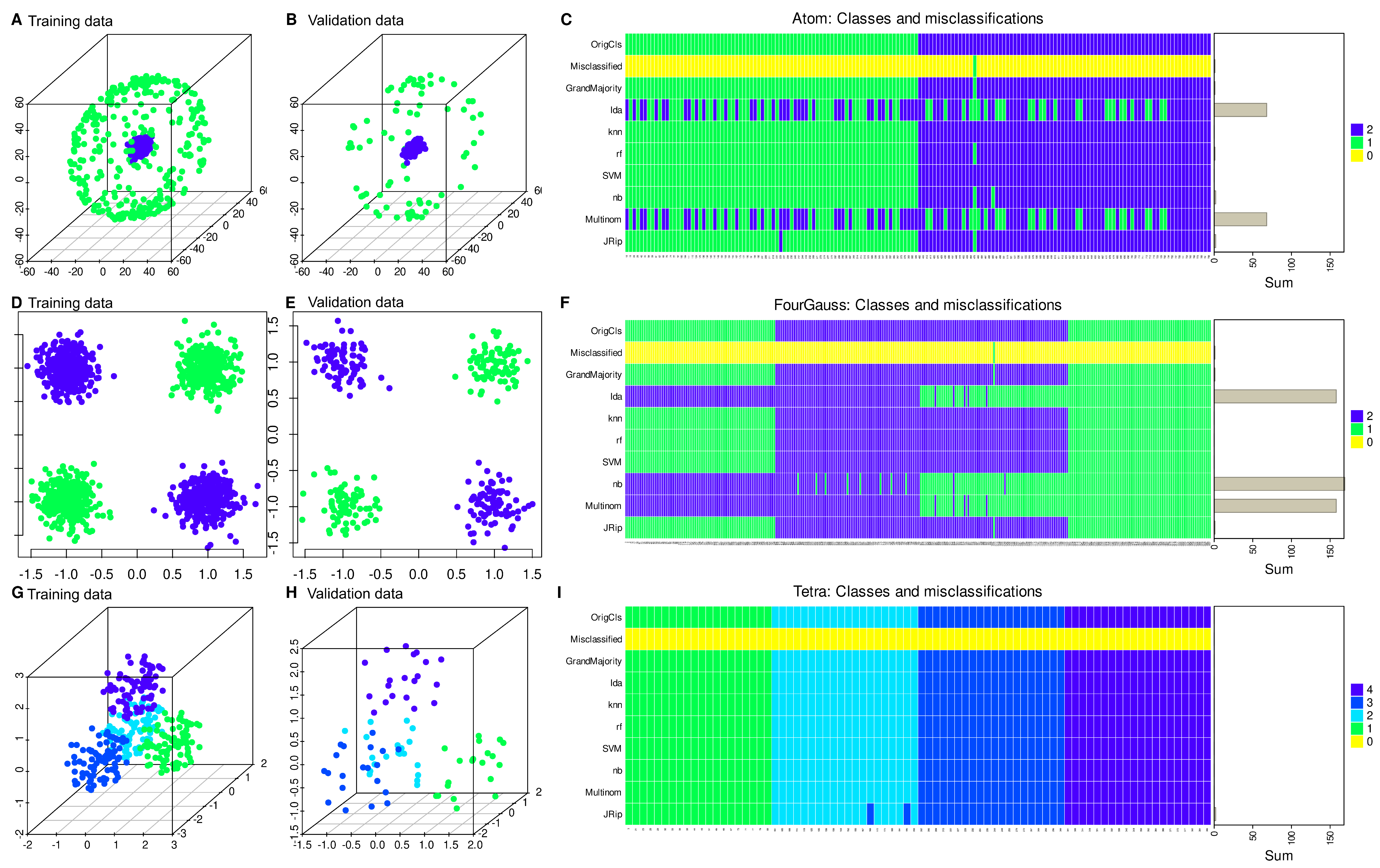
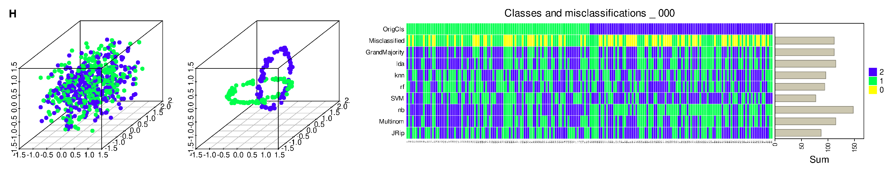
2.1. Sample Data Sets

The introductory example data set is an artificial data set published as part of the “Fundamental Clustering Problems Suite (FCPS)” [2]. It is freely available at https://www.mdpi.com/2306-5729/5/1/13/s1 (accessed on 14 August 2023) or in the similarly named R library “FCPS” (https://cran.r-project.org/package=FCPS [5], accessed on 14 August 2023). The “ChainLink” data set contains two distinct classes arranged as interlinked rings in the variables X, Y, and Z, each class containing n = 500 members. Two other data sets from the FCPS collection, “Atom” and “Tetra”, were additionally used. The “Atom” data set contains 3D data visually resembling an atomic nucleus and its shell, each composed of n = 200 data points. The “Tetra” data set consists of four classes of n = 100 points each, and each point has three variables indicating the position in a three-dimensional space and drawn independently and uniformly distributed. Additionally, a canonical machine learning data set was generated consisting of 4 normal distributions with means [(5,−5), (−5,5), (−5,−5), (5,5)] and standard deviations of 1 in both x and y directions with n = 400 observations in each Gaussian. This results in four heaps of points in an xy coordinate system. In both dimensions, the variables were normalized, i.e., standardized to mean 0 and unit variance. The upper left and lower right corners belong to class 1, and the lower left and upper right corners belong to class 2. This “Four Gaussians” data set provides a classic “XOR-structured" data set [6]. That is, in this two-dimensional group of data, one group is characterized by either high or low values in both variables. Otherwise, the case belongs to the other group.
A large biomedical data set was from multiomics data analysis in the context of non-small cell lung cancer [7]. The data set contained information from a total of n = 566 patients, including 672 differentially expressed mRNAs, 9 microRNAs, 719 gene methylation data, and 153 protein expression data. In the original study, spectral clustering was used to identify k = 5 clusters that correlated with patient survival. For the present analysis, we downloaded Supplementary Table S17 from the publication site at https://static-content.springer.com/esm/art%3A10.1038%2Fs41598-023-31426-w/MediaObjects/41598_2023_31426_MOESM2_ESM.xlsx (accessed on 14 August 2023). The file contains cluster membership information and preprocessed omics data used by the authors of the original paper to train and validate machine-learning-based classifiers. In the present demonstration, the data set was used to test the sufficiency of regression as an analysis method of biomedical data sets compared to alternative methods, with no intention to replicate or challenge the published results.

2.2. Experimentation

Software coding was done in the R [8] and Python [9] languages on Linux. The main packages were “caret” (https://cran.r-project.org/package=caret (accessed on 14 August 2023) [10]) for R and “scikit-learn” (https://scikit-learn.org/stable/ (accessed on 14 August 2023) [11]) for Python. Figures were created using the R libraries “ggplot2” (https://cran.r-project.org/package=ggplot2 (accessed on 14 August 2023) [12]), “scatterplot3d” (https://cran.r-project.org/package=scatterplot3d (accessed on 14 August 2023) [13]), “ComplexHeatmap” (https://www.bioconductor.org/packages/ComplexHeatmap/ (accessed on 14 August 2023) [14]), “cvms” (https://cran.r-project.org/package=cvms (accessed on 14 August 2023) [15]), and “nnet” (https://cran.r-project.org/package=nnet (accessed on 14 August 2023) [16]) in R, or the seaborn statistical data visualization package (https://seaborn.pydata.org (accessed on 14 August 2023) [17]) in Python. A set of algorithms covering various machine learning and statistical approaches was trained on an 80% training sample of the data set.
The algorithms included regression methods, specifically binary or multinomial logistic regression for data sets with k = 2 or k > 2 classes, respectively. Additionally, linear discriminant analysis (LDA) [18], a commonly applied statistical procedure, was employed. Furthermore, a non-compressive collection of supervised machine learning algorithms was utilized consisting of methods often used for biomedical data analysis and generally known to perform classification tasks well. These included random forest [4] as a robust tree-based bagging classifier, support vector machine (SVM) [19] as a hyperplane separation-based method, k-nearest neighbors [20] as a distance-based classifier, and naïve Bayes [21] as a posterior probabilities-based method. In addition, decision rules were created based on repeated incremental clipping for error reduction (RIPPER [22]). Hyperparameter tuning, such as kernel shape for SVM, number of trees for random forest, and others, was done in a grid search, and classifier training and validation were done using nested cross-validation. Details of the R code are available at https://github.com/JornLotsch/MisClassificationRegressionNN/blob/main/MisClassificationAnaylsis_MainFunctions_paper.R (accessed on 14 August 2023).
The methods were then compared in terms of their classification performance based on balanced accuracy [23] in a 20% hold-out validation sample separated from the data set before the analysis. In addition, the area under the receiver operator curve (roc-auc) was calculated [24]. A “mixture of experts” approach was used to identify the most suitable variables based on the best-performing classification algorithms. These were identified by item categorization into subsets labeled “A”, “B”, and “C”, implemented as computed ABC analysis (cABC) [25]. Algorithms falling in category “C”, which is generally considered as “the trivial many” [26], were rejected as a basis of variable selection. The informative variables were then selected for the best models using generic permutation importance as a feature selection method applicable to any type of classifier.
Since this was not a feature selection benchmarking assessment, other methods (for an overview, see [27]) were not considered. Finally, the selected variables were used to train algorithms in a 5 × 20 nested cross-validation scenario using randomly selected subsets of 67% of the original training data set and applied to each 80% of the hold-out validation data subset.

3. Results

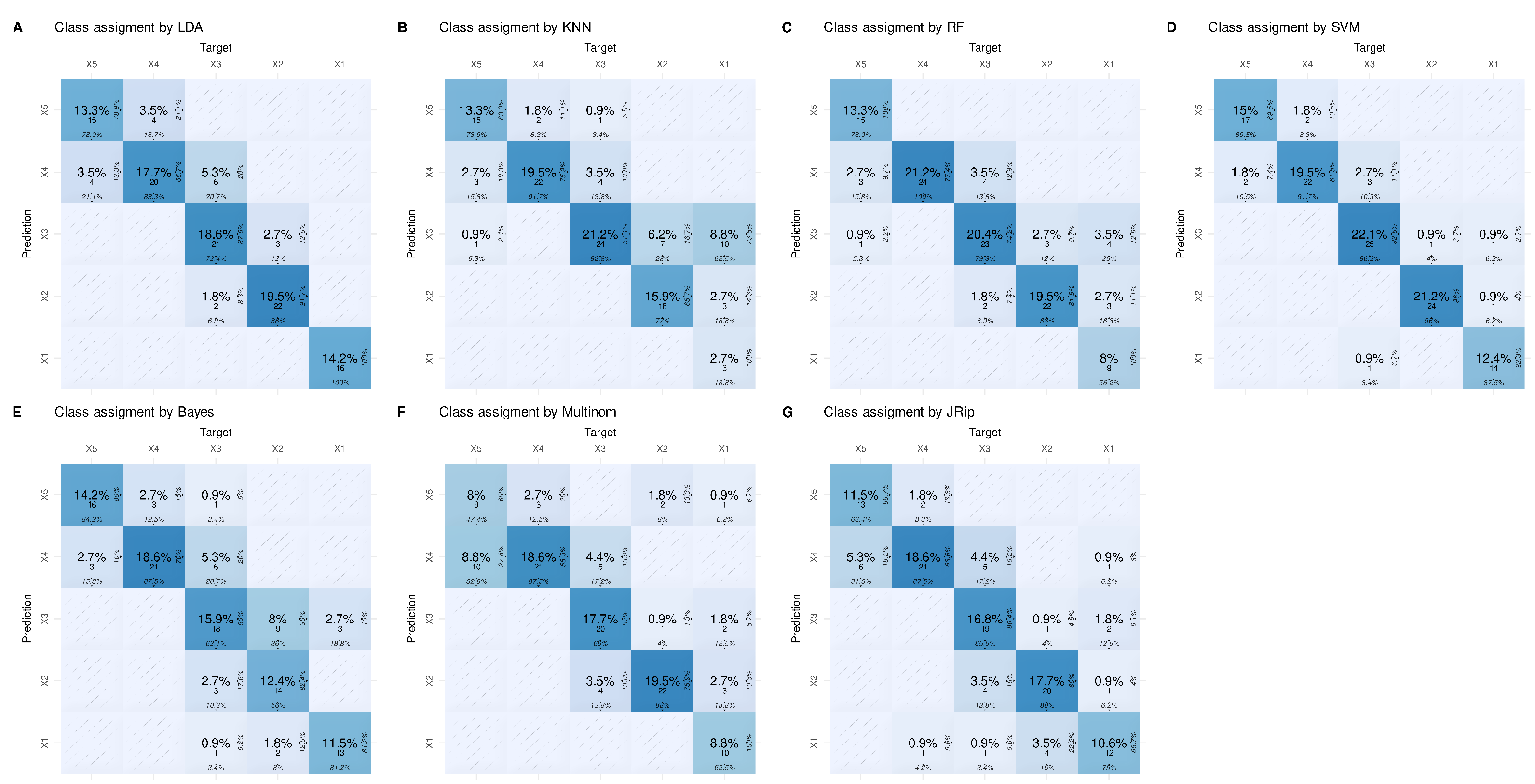
3.1. Regression Occasionally Generalizes Poorly Compared to Alternative Methods

As shown in the introductory example, the regression result for the variable “Y” in the “ChainLink” data set was highly statistically significant (Table 1). However, cautious interpretation is needed when considering “Y” as the primary determinant of class membership since regression had only a modest ability to assign class membership of new cases not seen during regression model building (Figure 1).
To further validate this, six different models were trained on all possible combinations of preserved and randomly permuted variables (Figure 2). The results showed that most algorithms successfully classified unseen data when trained on the three variables, with regression and LDA performing worst as mentioned in the introductory example. By contrast, classification constantly failed when all variables were randomly permuted as the expected outcome in this scenario (Figure 2G,H, respectively). Surprisingly when considering the statistical results of regression analysis, training with only the variable “Y”, i.e., the variable emerging as a highly significant result from regression analysis, resulted in poor classification performance for new data across all algorithms (Figure 2B).
Regression was also found to be inferior to machine learning algorithms in the FCPS-based “Atom” data set and in the “Four Gaussians” data set (Figure 3). However, to highlight that regression can be a successful method, the FCPS-based “Tetra” data set was included where, as expected, regression provided a perfect classification similar to the other methods (Figure 3).
The weakness of regression was not arbitrarily produced by the actual choice of artificial data sets expected to pose problems but extends to real-life data sets, such as a large multiomics data set from cancer research (Figure 4).
There, for example, support vector machine outperformed regression considerably. This data set once again identified regression as one of the weakest predictors producing the least accurate class assignment of unseen (validation) cases (Figure 5).

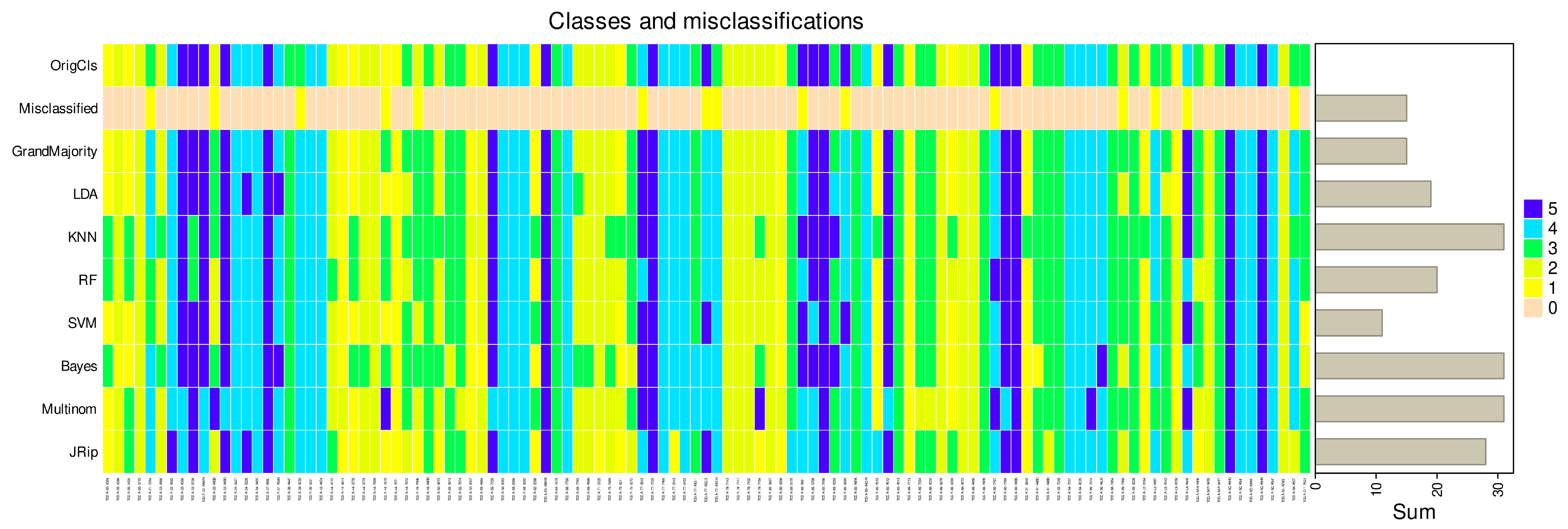
3.2. Regression Inadequately Captures the Structural Characteristics of Certain Data Sets

In the “Four Gaussians” data set, regression analysis failed to provide the correct classification when the classes in the data set are linearly non-separable (Figure 6E,F). Its inability to draw a line between the two original classes was shared by a single-layer neural network (Figure 6A). The balanced accuracy obtained with binary logistic regression or with a single-layer perceptron was about 50%, i.e., guessing level in two classes. Only the addition of a hidden layer with at least one and up to three neurons (Figure 6B–D) enabled the algorithms to perform the classification successfully, eventually reaching 100% accuracy. When the class labels were changed so that the classes were linearly separable (Figure 6G), both regression and simple artificial neural networks were able to perform classification with 100% accuracy (Figure 6H). The R code for this experiment is available at https://github.com/JornLotsch/MisClassificationRegressionNN (accessed on 14 August 2023).

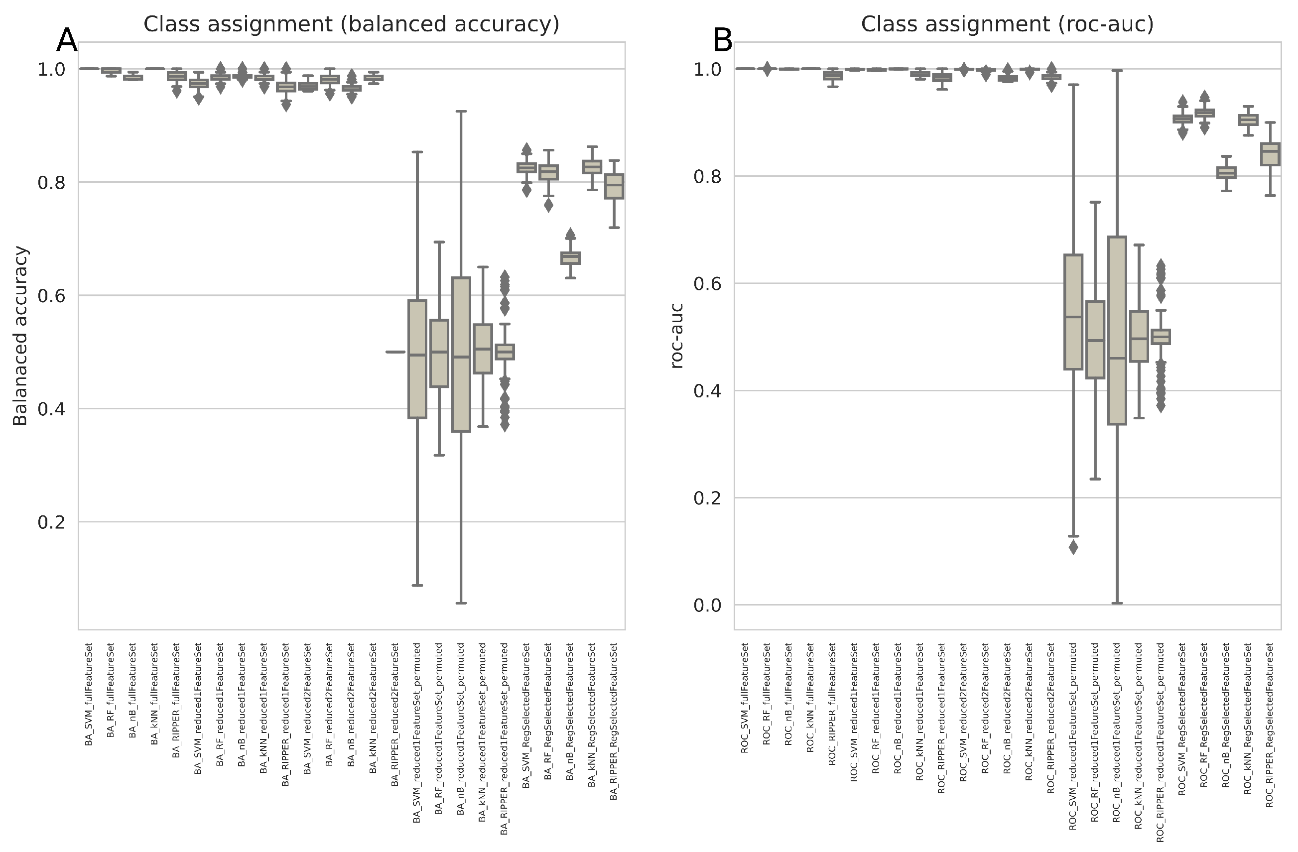
3.3. Variables Chosen by the Most Successful Algorithms Are More Generalizable

The above experiments cast doubt on the validity of the statistically significant result of the logistic regression analysis identifying the variable “Y” in the FCPS “ChainLink” data set as the relevant variable for class assignment. Regression was the poorest model for assigning new cases to the correct classes based on the available variables, and, therefore, may not be the most reliable “expert” to indicate which variables are relevant in the data set. Using cABC analysis and the permutation importance method on the balanced accuracy, LDA and regression were placed in category “C” by cABC analysis, indicating that these methods provided the poorest description of the “ChainLink” data set and should, therefore, not be explored further for important variables (Figure 7).
The brute force experiment reported above suggested that variable “Y” was consistently worse than other combinations as a basis for training any model to perform the classification task on new data.
When this issue was addressed using feature selection based on permutation variable importance, variable “X” was consistently found to be important for most of the (well-performing) algorithms, while “Y” and “Z” were each important for three out of five algorithms (Figure 8), which was further addressed by testing classifiers when trained with different combinations of variables. Training of the models with all three variables resulted in perfect classification by support vector machine, random forest, and k-nearest neighbors (median balanced accuracy = 1; Figure 9). When combinations of “XZ” or “XY” were used, the median balanced accuracy was still 0.98 or higher for all algorithms (Figure 9). More importantly, the use of only the variable “Y” for training, i.e., the variable that had emerged from the regression analysis as the only significant variable for a class assignment in this data set, resulted in significantly worse classification performance on new data, with balanced accuracies ranging from 0.67 for the naïve Bayesian classifier to 0.83 for the k-nearest neighbors classifier.
When applying proposed interpretations of accuracy values as good or bad, such as the rule of thumb of 0.5 = no discrimination, 0.5–0.7 = poor discrimination, 0.7–0.8 = acceptable discrimination, 0.8–0.9 = excellent discrimination, and >0.9 = outstanding discrimination [28], the drop in accuracy means that the classification dropped one or two categories when using the results of regression as a selection criterion for informative variables. Thus, the “advice” from the regression analysis turned out to be bad advice, and better algorithms were available that gave much better “advice” about which variables were important in the data set. As reported in the introductory example at the beginning of this work, binary logistic regression produced an accuracy of 0.65 on this data set. Therefore, the variable indicated as most important by this poor classifier turned out to be suboptimal, as expected, emphasizing the need to take into account the variables indicated by the best classifiers. As a control, training of the algorithms with permuted and, therefore, nonsensical information led, as expected, to a balanced accuracy in the median around 0.5 or 50%, which is the expected guessing level and, therefore, supports that the observed correct classifications in the other training scenarios are not due to overfitting or other technical errors in the Python code implementations of the present experiment.
In the real-life multiomics data set, the highest balanced accuracies of the k = 5 classes identified by the authors of the original paper [7] were achieved with support vector machine, along with random forest, k-nearest neighbors, LDA, and RIPPER (Figure 7). In fact, the first two algorithms currently identified as the best (SVM, random forest) were used by the authors of the original report [7]. Thus, from the range of methods available, these should be used to identify the variables relevant to the cluster structure in this data set. This will not be done again here, as it is not the intention of this report to verify the original results, but rather to use this data set as an example to discourage reliance on regression alone in this type of data set.

4. Discussion

The present findings challenge the traditional reliance on regression as the standard for multivariate data analysis in biomedical research aimed at identifying variables most relevant for a given class structure. The widespread use of regression (for a comprehensive overview, see [29]) in the past may have been due to the lack of alternatives or computational limitations. However, with the advancement of machine learning techniques and the availability of computational power, it is now possible to employ a collection of different methods for data analysis and select those that accurately capture the underlying structure of the data.
This paper attempts to clarify a common misconception about regression, namely that regression algorithms for classification are as powerful as machine learning methods and suffice for the analysis of biomedical data. This is not true. By contrast, this paper points out a structural weakness of regression in separating classes in data sets, comparable to early neural networks. The breakthrough in addressing linearly non-separable classifications of data sets was the introduction of hidden layers. In this context, regression provides the equivalent of a simple perceptron, which, with good reason, has been discarded for data analysis in favor of more sophisticated model architectures. One can show that a single artificial neuron of a neural network can be described as nonlinear (logistic) regression and vice versa. However, to generalize this to “machine learning is nothing more than the application of regression models under a different name” is a mistake. Regression models can handle the same type of classification problems as neural networks without hidden layers. This type of model was proposed by Rosenblatt in 1958 under the name “Perceptron” [30]. These algorithms were used until 1970 for many problems, including classification. In 1969, Minsky and Papert published a book showing that single-layer neural networks are, in principle, incapable of classifying data sets that are linearly non-separable [6].
The data set “Four Gaussians” (Figure 6) illustrates this property for empirical data in a nutshell: for this type of data set, there is no single straight line, i.e., a “hyperplane in two dimensions”, that can correctly separate the two classes. Regression models used for classification (e.g., logistic regression) can only achieve a classification accuracy of about 50%, i.e., guessing level. Current experiments emphasize that regression is equivalent to a simple perceptron with respect to classification. A practical example of such data is a normal versus abnormal body mass index (BMI) comparison: a person is in the “normal BMI” (the green group in Figure 6) group if they have either a high weight and height or a low weight and height, otherwise they are in the “abnormal BMI” group (the blue group in Figure 6).
The reason for the inability of (logistic) regression to solve “XOR-structured” problems can be deduced from its formula. Let p(x)∼0 denote that a case with a given value x belongs to one class and p(x)∼1 that the case belongs to the other class of a dichotomy. Then, logistic regression is described by the formula
p ( x ) = 1 / ( 1 + e ( β 0 + β 1 x ) )
where β 0 is the intercept and β 1 the slope of a line (= hyperplane in a multivariate setting). The further away from the decision hyperplane, the closer the values of p(x) are to 0 or 1, respectively. In summary, both regression and logistic regression are limited to a single hyperplane decision, regardless of how the parameters ( β 0 and β 1 ) are optimized. It is clear that these types of classifiers can never solve “XOR-structured” problems.
Thus, regression models, which are computationally equivalent to neural networks with one layer, are in principle unable to classify data sets that are linearly non-separable. Indeed, the other algorithms used in this report, except LDA, could classify the “Four Gaussians” data set (Figure 3D–F). However, testing whether a given empirical multivariate data set is linearly non-separable is not an easy task and often requires the use of more powerful machine learning algorithms [31]. A simple example demonstrating this is the “ChainLink” data set used in the present experiments (see introductory example and Figure 2). Machine learning (ML) models such as deep learning, i.e., hidden layer networks, support vector machine (SVM ), random forest, and other ML algorithms can easily handle linearly non-separable data. Some of them, such as SVM, are specifically designed to handle linearly non-separable classification problems.
The current experiments have shown that relying on a single algorithm to select informative variables in a data set has potential risks in scientific findings. If the chosen algorithm fails for any reason to capture the class structure, although statistics may deliver highly significant p-values the results could be unreliable. Regression can be successful, as in the “Tetra” data set and many others reported in the scientific literature, however, this should not be assumed as a given fact but verified in every actual data set. The present workflow included alternative methods creating a “mixture of experts” on which conclusions can be relied with greater confidence than on a single model that has not even been tested in unseen data, as it is a frequent approach in biomedical research. This is likely to provide a result closer to the ground truth than when relying on a single model and basing research results on a particular model architecture. Furthermore, adding further methods provides internal validation, and there is no major disadvantage compared to a pure regression analysis.
However, the abandonment of an apparent standard that provided reassurance about the results of data analysis could be perceived as a disadvantage. In fact, selecting relevant variables requires more effort than simply accepting the statistical results of a regression. There are many methods for selecting features, of which the permutation importance method chosen here is only one [27]. These include univariate feature selection methods such as effect size calculations, the false positive rate, the family-wise error rate, selection of the k best variables based on F-statistics, and others, available, for example, in the “sklearn.feature_selection” module of the “scikit-learn” Python package (https://scikit-learn.org/stable/modules/feature_selection.html (accessed on 14 August 2023) [11]). Model-based methods are applied after training the algorithms and include methods such as “SelectFromModel” (SFM), which selects features based on importance weights in the trained algorithm, and Recursive Feature Elimination (RFE), which selects features by recursively considering smaller and smaller feature sets and generating a feature ranking, and many others. Neural-network-based feature selection was not even considered in these experiments [32].
The choice of algorithms also influences the final result. Currently, algorithms of different types have been compiled, but alternatives are certainly possible. In addition, as shown in a simple biomedical case [33], the current setting of the hyperparameters can directly affect the classification performance and thus, the ranking of the algorithms, resulting in different sets of algorithms from which to derive the relevant features. While this may be a difficult task to test, reverting to a simple single method, with the uncertainty of whether it even captures the class structure in a data set, does not seem to be a better solution.
The mixture of experts makes the model predictions more robust. In the present experiments, a majority vote was included in the graphical presentation of results (“grand majority” columns in Figure 2, Figure 3 and Figure 4), showing that the occasional weakness of one or the other model can often be compensated by the votes contributed by stronger models although this might not be a general rule. In fact, research has shown that using a “mixture of experts” (MOE) approach, where multiple models are combined, can yield more accurate results in the analysis of biomedical data. In the cited multiomics example paper, support vector machine, random forest, and additionally, a feed-forward neural network were used [7], but not regression. This is consistent with the present observations and the referenced examples. Further examples include a customized electrocardiogram (ECG) beat classifier combined with a global classifier to form a MOE classifier structure that also provided significant performance improvement over single method approaches [34]. Similarly, a wide variety of machine learning algorithms to select the best combination of biomarkers to predict categorical outcomes from highly unbalanced (biomedical) data sets has been proposed [35,36,37], and our own molecular research also points to the advantage of using multiple models. Regression can be one of the used models but it should not be the only one [38].
This paper is not intended as a comprehensive comparative evaluation of approaches to classify data sets. Other approaches than MOE are available for classification and/or feature selection on complexly structured data sets [39]. Feature selection can also based on deep learning models, which seems promising but requires data sets that are usually larger than those addressed here [40]. Since the goal of this paper is to show that regression alone is not a sufficient method due to its weaknesses, it would be beyond the scope of this paper to analyze all proposed alternatives in a comparative way. This paper proposes a reconsideration of the insistence on analyzing biomedical data sets only with regression and to broaden the range of methods towards algorithms that better capture the actual structure of the data sets. However, any proposal to replace regression with deep learning would be going too far.

5. Conclusions

Regression is only one of several possible mathematical models to describe a data set; it can be valid, as in the present “Tetra” data set, but this cannot be taken for granted and used to demand that scientific reports have to be based on regression analysis. Regression is not always the best and most correct model, as shown in other data sets where it failed, as in three artificial data sets, or was one of the poorest predictors in an actual real-life multiomics data set from cancer research. Regression has been outperformed by most machine-learning-based algorithms on almost every data set. A regression model needs to be validated like any other model, although many scientific papers do not do this, so it cannot be taken for granted that the results reported are valid. In contrast, this paper highlights a structural problem with logistic regression that it has in common with early neural network architectures (perceptrons), which were abandoned with good reason. Since it is difficult or even impossible to judge whether a given real-life data set is linearly non-separable, this paper suggests a mixture of experts (MOE) of machine learning models, which may include regression, to handle classification problems in biomedical data. To ensure accurate analysis of biomedical data sets, it is critical to recognize and address the limitations of regression analysis, which can occasionally produce inaccurate results. Therefore, it is highly recommended to avoid relying solely on regression analysis when examining biomedical data sets. By incorporating additional analytical approaches, researchers can mitigate the weaknesses of regression analysis and obtain more reliable results.

Author Contributions

J.L.—Conceptualization of the project, programming, performing the experiments, writing of the manuscript, data analyses, and creation of the figures, funding acquisition. A.U.—Theoretical background, mathematical implementation, writing of the manuscript. All authors have read and agreed to the published version of the manuscript.

Funding

J.L. was supported by the Deutsche Forschungsgemeinschaft (DFG LO 612/16-1).

Institutional Review Board Statement

Not applicable. All data sets have been taken from public sources.

Informed Consent Statement

Not applicable. All data sets have been taken from public sources.

Data Availability Statement

Data sets except the “Four Gaussians” example have been taken from public sources that are precisely referenced in the report. The data of the “Four Gaussians” example and the R code for this experiment are available at https://github.com/JornLotsch/MisClassificationRegressionNN (accessed on 14 August 2023). Please note that the unmodified R code runs only on Unix-like systems (e.g., Linux, MacOS) due to the particular kind of implementation of parallel processing.

Conflicts of Interest

The authors declare no conflict of interest. The funders had no role in the design of the study; in the collection, analyses, orinterpretation of data; in the writing of the manuscript; or in the decision to publish the results.

References

  1. Lo, A.; Chernoff, H.; Zheng, T.; Lo, S.H. Why significant variables are not automatically good predictors. Proc. Natl. Acad. Sci. USA 2015, 112, 13892–13897. [Google Scholar] [CrossRef] [PubMed]
  2. Ultsch, A.; Lötsch, J. The Fundamental Clustering and Projection Suite (FCPS): A Dataset Collection to Test the Performance of Clustering and Data Projection Algorithms. Data 2020, 5, 13. [Google Scholar] [CrossRef]
  3. Pearson, K. LIII. On lines and planes of closest fit to systems of points in space. Lond. Edinb. Dublin Philos. Mag. J. Sci. 1901, 2, 559–572. [Google Scholar] [CrossRef]
  4. Breiman, L. Random Forests. Mach. Learn. 2001, 45, 5–32. [Google Scholar] [CrossRef]
  5. Thrun, M.; Stier, Q. Fundamental clustering algorithms suite. SoftwareX 2021, 13, 100642. [Google Scholar]
  6. Minsky, M.; Papert, S. Perceptrons: An Introduction to Computational Geometry; MIT Press: Cambridge, MA, USA, 1969. [Google Scholar]
  7. Khadirnaikar, S.; Shukla, S.; Prasanna, S.R.M. Machine learning based combination of multi-omics data for subgroup identification in non-small cell lung cancer. Sci. Rep. 2023, 13, 4636. [Google Scholar] [CrossRef]
  8. Ihaka, R.; Gentleman, R. R: A Language for Data Analysis and Graphics. J. Comput. Graph. Stat. 1996, 5, 299–314. [Google Scholar] [CrossRef]
  9. Van Rossum, G.; Drake, F.L., Jr. Python Tutorial; Centrum voor Wiskunde en Informatica Amsterdam: Amsterdam, The Netherlands, 1995; Volume 620. [Google Scholar]
  10. Kuhn, M. Building Predictive Models in R Using the caret Package. J. Stat. Softw. 2008, 28, 1–26. [Google Scholar] [CrossRef]
  11. Pedregosa, F.; Varoquaux, G.; Gramfort, A.; Michel, V.; Thirion, B.; Grisel, O.; Blondel, M.; Prettenhofer, P.; Weiss, R.; Dubourg, V.; et al. Scikit-learn: Machine Learning in Python. J. Mach. Learn. Res. 2011, 12, 2825–2830. [Google Scholar]
  12. Wickham, H. ggplot2: Elegant Graphics for Data Analysis; Springer: New York, NY, USA, 2009. [Google Scholar]
  13. Ligges, U.; Mächler, M. Scatterplot3d–An R Package for Visualizing Multivariate Data. J. Stat. Softw. 2003, 8, 1–20. [Google Scholar] [CrossRef]
  14. Gu, Z.; Eils, R.; Schlesner, M. Complex heatmaps reveal patterns and correlations in multidimensional genomic data. Bioinformatics 2016, 32, 2847–2849. [Google Scholar] [CrossRef]
  15. Olsen, L.R.; Zachariae, H.B. cvms: Cross-Validation for Model Selection. 2023. Available online: https://cran.r-project.org/package=cvms (accessed on 14 August 2023).
  16. Venables, W.N.; Ripley, B.D. Modern Applied Statistics with S, 4th ed.; Springer: New York, NY, USA, 2002; ISBN 0-387-95457-0. [Google Scholar]
  17. Waskom, M.L. Seaborn: Statistical data visualization. J. Open Source Softw. 2021, 6, 3021. [Google Scholar] [CrossRef]
  18. Fisher, R.A. The use of multiple measurements in taxonomic problems. Ann. Eugen. 1936, 7, 179–188. [Google Scholar] [CrossRef]
  19. Cortes, C.; Vapnik, V. Support-Vector Networks. Mach. Learn. 1995, 20, 273–297. [Google Scholar] [CrossRef]
  20. Cover, T.; Hart, P. Nearest neighbor pattern classification. IEEE Trans. Inf. Theor. 1967, 13, 21–27. [Google Scholar] [CrossRef]
  21. Bayes, M.; Price, M. An Essay towards Solving a Problem in the Doctrine of Chances. By the Late Rev. Mr. Bayes, F. R. S. Communicated by Mr. Price, in a Letter to John Canton, A. M. F. R. S. Philos. Trans. 1763, 53, 370–418. [Google Scholar] [CrossRef]
  22. Cohen, W.W. Fast Effective Rule Induction. In Machine Learning Proceedings 1995, Proceedings of the Twelfth International Conference on Machine Learning, Tahoe City, California, 9–12 July 1995; Prieditis, A., Russell, S., Eds.; Morgan Kaufmann: San Francisco, CA, USA, 1995; pp. 115–123. [Google Scholar] [CrossRef]
  23. Brodersen, K.H.; Ong, C.S.; Stephan, K.E.; Buhmann, J.M. The Balanced Accuracy and Its Posterior Distribution. In Proceedings of the 2010 20th International Conference on Pattern Recognition (ICPR), Istanbul, Turkey, 23–26 August 2010; pp. 3121–3124. [Google Scholar] [CrossRef]
  24. Peterson, W.; Birdsall, T.; Fox, W. The theory of signal detectability. Trans. Ire Prof. Group Inf. Theory 1954, 4, 171–212. [Google Scholar] [CrossRef]
  25. Ultsch, A.; Lötsch, J. Computed ABC Analysis for Rational Selection of Most Informative Variables in Multivariate Data. PLoS ONE 2015, 10, e0129767. [Google Scholar] [CrossRef]
  26. Juran, J.M. The non-Pareto principle; Mea culpa. Qual. Prog. 1975, 8, 8–9. [Google Scholar]
  27. Guyon, I. An introduction to variable and feature selection. J. Mach. Learn. Res. 2003, 3, 1157–1182. [Google Scholar]
  28. Hosmer, D.; Lemeshow, S.; Sturdivant, R. Applied Logistic Regression; Wiley Series in Probability and Statistics; Wiley: Hoboken, NJ, USA, 2013. [Google Scholar]
  29. Fahrmeir, L.; Kneib, T.; Lang, S.; Marx, B. Regression: Models, Methods and Applications; Springer: Berlin/Heidelberg, Germany, 2013. [Google Scholar]
  30. Rosenblatt, F. The perceptron: A probabilistic model for information storage and organization in the brain. Psychol. Rev. 1958, 65, 386–408. [Google Scholar] [CrossRef]
  31. Elizondo, D. The linear separability problem: Some testing methods. IEEE Trans. Neural Netw. 2006, 17, 330–344. [Google Scholar] [CrossRef] [PubMed]
  32. Verikas, A.; Bacauskiene, M. Feature selection with neural networks. Pattern Recognit. Lett. 2002, 23, 1323–1335. [Google Scholar] [CrossRef]
  33. Lötsch, J.; Mayer, B. A Biomedical Case Study Showing That Tuning Random Forests Can Fundamentally Change the Interpretation of Supervised Data Structure Exploration Aimed at Knowledge Discovery. BioMedInformatics 2022, 2, 544–552. [Google Scholar] [CrossRef]
  34. Hu, Y.H.; Palreddy, S.; Tompkins, W.J. A patient-adaptable ECG beat classifier using a mixture of experts approach. IEEE Trans. Biomed. Eng. 1997, 44, 891–900. [Google Scholar] [CrossRef] [PubMed]
  35. Leclercq, M.; Vittrant, B.; Martin-Magniette, M.L.; Scott Boyer, M.P.; Perin, O.; Bergeron, A.; Fradet, Y.; Droit, A. Large-Scale Automatic Feature Selection for Biomarker Discovery in High-Dimensional OMICs Data. Front. Genet. 2019, 10, 452. [Google Scholar] [CrossRef]
  36. Miettinen, T.; Nieminen, A.I.; Mäntyselkä, P.; Kalso, E.; Lötsch, J. Machine Learning and Pathway Analysis-Based Discovery of Metabolomic Markers Relating to Chronic Pain Phenotypes. Int. J. Mol. Sci. 2022, 23, 5085. [Google Scholar] [CrossRef]
  37. Kringel, D.; Kaunisto, M.A.; Kalso, E.; Lötsch, J. Machine-learned analysis of global and glial/opioid intersection-related DNA methylation in patients with persistent pain after breast cancer surgery. Clin. Epigenetics 2019, 11, 167. [Google Scholar] [CrossRef]
  38. Lötsch, J.; Schiffmann, S.; Schmitz, K.; Brunkhorst, R.; Lerch, F.; Ferreiros, N.; Wicker, S.; Tegeder, I.; Geisslinger, G.; Ultsch, A. Machine-learning based lipid mediator serum concentration patterns allow identification of multiple sclerosis patients with high accuracy. Sci. Rep. 2018, 8, 14884. [Google Scholar] [CrossRef]
  39. Statnikov, A.; Henaff, M.; Narendra, V.; Konganti, K.; Li, Z.; Yang, L.; Pei, Z.; Blaser, M.J.; Aliferis, C.F.; Alekseyenko, A.V. A comprehensive evaluation of multicategory classification methods for microbiomic data. Microbiome 2013, 1, 11. [Google Scholar] [CrossRef]
  40. Li, K.; Wang, F.; Yang, L.; Liu, R. Deep feature screening: Feature selection for ultra high-dimensional data via deep neural networks. Neurocomputing 2023, 538, 126186. [Google Scholar] [CrossRef]
Figure 1. Weakness of the regression model fit on 80% of the data (training) to predict the remaining 20% of the data (validation) of the FCPS-based “ChainLink” data set. (A): Training data set. (B): Validation data set. (C): Confusion matrix plot of the assignment to each of the k = 2 classes using the regression model. In the center of each tile is the normalized number (total percentage) of cases assigned to each class, and below is the number of cases per class. The column-wise percentages are shown at the bottom, and the row-wise percentages are shown to the right of each tile. (D): Confusion matrix plot for the results when assigning a trained random forest model instead of the regression model. (E): Matrix heat plot of the class assignment of unseen cases (20% hold-out validation sample) by either regression or random forest trained on 80% of the data set. For comparison, the original class assignments are shown in the top row.
Biomedinformatics 03 00054 g001
Figure 2. Comparative class assignment error rates for unseen cases (20% hold-out validation sample) of the FCPS-based “ChainLink” data set by d = 6 different classifiers trained on 80% of the respective data sets (lda = linear discriminant analysis, knn = k-nearest neighbors, rf = random forest, SVM = support vector machine, nb = naïve Bayes, multinom = logistic regression, binary for k = 2 classes, jRip = repeated incremental clipping for error reduction). An exhaustive approach of permutations of 1–3 variables was used to identify the variables on which the class assignment can best be based. The panels AH show the different different scenarios, with a three-dimensional visualization of the actual training data set training data set on the left, the validation data set in the middle panel, and the classification results on this validation data set based on training with the training data set on the right. Which variables were permuted or not in each panel is coded in the titles of the matrix heat plots as 0 or 1, e.g., “111” (panel G) means all variables in original form, “000” (panel H) all permuted, “010” (panel B) only the 2nd of three variables, i.e., “Y”, permuted, and so on. For comparison, the original class assignments are shown in the top row, the number of finally misclassified cases is shown in the second row, based on the majority vote of all d = 6 classifiers shown in the third row.
Biomedinformatics 03 00054 g002aBiomedinformatics 03 00054 g002b
Figure 3. Comparative class assignment error rates for unseen cases (20% hold-out validation sample) by d = 6 different classifiers trained with 80% of the respective data sets (lda = linear discriminant analysis, knn = k-nearest neighbors, rf = random forest, SVM = support vector machine, nb = naïve Bayes, Multinom = logistic regression, binary for k = 2 classes and multinomial for k > 2 classes, jRip = repeated incremental clipping for error reduction). (A): Training data from the FCPS-based “Atom” data set. (B): Validation data. (C): Matrix heat plot of the class assignment of unseen cases in the hold-out validation sample. For comparison, the original class assignments are shown in the top row, the number of finally misclassified cases is shown in the second row, based on the majority vote of all d = 6 classifiers shown in the third row. (DF): As panels (AC) but for the (standardized) “Four Gaussians” data set. (GI): As panels (AC) but for the FCPS-based “Tetra” data set.
Biomedinformatics 03 00054 g003
Figure 4. Multiomics data set [7]: Comparative class assignment error rates for unseen cases (20% hold-out validation sample) by d = 6 different classifiers trained with 80% of the respective data sets (lda = linear discriminant analysis, knn = k-nearest neighbors, rf = random forest, SVM = support vector machine, nb = naïve Bayes, Multinom = multinomial logistic regression, for k = 5 classes, jRip = repeated incremental clipping for error reduction). Matrix heat plot of the class assignment of unseen cases in the hold-out validation sample. For comparison, the original class assignments are shown in the top row, the number of finally misclassified cases is shown in the second row, based on the majority vote of all d = 6 classifiers shown in the third row.
Biomedinformatics 03 00054 g004
Figure 5. Multiomics data set [7]: Confusion matrix plot of the assignment to each of the k = 2 classes using the logistic regression model. In the center of each tile is the normalized number (total percentage) of cases assigned to each class, and below is the number of cases per class. The column-wise percentages are shown at the bottom, and the row-wise percentages are shown to the right of each tile. (A): LDA = linear discriminant analysis, (B): KNN = k-nearest neighbors, (C): RF = random forest, (D): SVM = support vector machines, (E): Bayes = naïve Bayes, (F): Multinom = logistic regression, (multinomial for k = 5 classes), (G): JRip = repeated incremental clipping for error reduction.
Biomedinformatics 03 00054 g005
Figure 6. Structural limitations of regression to separate classes in a data set, exemplified by the “Four Gaussians” data (standardized). (AD): Neural network architectures with 0–3 neurons in a hidden layer (N0–N3). (E): Original two-class data set. (F): Balanced accuracies obtained on a 20% hold-out validation sample after training the algorithms in a 100-fold cross-validation scenario. The box plots show the median and the 25th and 75th percentiles and are overlaid with individual balanced accuracies as single points. (G): Data set switched to a simpler problem. (H): Balanced accuracies obtained by running the same code used in panel F on the data set in panel (G).
Biomedinformatics 03 00054 g006
Figure 7. Identification of the best algorithms based on the balanced accuracy (BA) of class assignment for unseen cases (20% hold-out validation sample) by d = 6 different classifiers trained with 80% of the respective data sets (lda = linear discriminant analysis, knn = k-nearest neighbors, rf = random forest, SVM = support vector machine, nb = naïve Bayes, Mutinom = logistic regression, (multinomial for k = 5 classes, jRip = repeated incremental clipping for error reduction). (A): Item categorization via cABC analysis of the balanced accuracies in the FCPS-based “ChainLink” data set. The ABC plots (blue lines) show the cumulative distribution function of the importance variables together with the identity distribution, xi = constant (magenta line), and the uniform distribution, i.e., as a stopping criterion for the repetitions of the cABC analysis. The red lines show the boundaries between the ABC subsets “A”, “B”, and “C”. (B): Bar plot of the performance measures, quantified as balanced accuracy, of the d = 6 algorithms. (C,D): Similar to panels (A,B) but for the real-life multiomics data set [7].
Biomedinformatics 03 00054 g007
Figure 8. Feature selection for the FCPS-based “ChainLink” data set, using the d = 4 best performing classification algorithms, with generic permutation importance and balanced accuracy as the criterion. (AE): Bar plots of permutation features importance (variables “X1”, “X2”, “X3” corresponding to the x, y, and z coordinates of the three-dimensional data set, resulting from different classifiers as indicated at the x-axis legends (kNN = k-nearest neighbors, SVM = support vector machine, nBayes = naïve Bayes, RF = random forest, RIPPER = repeated incremental clipping for error reduction). (FJ): Corresponding ABC plots of feature importance. Variables in sets “A” or “B” were retained for the majority vote. The ABC plots (blue lines) show the cumulative distribution function of the importance variables together with the identity distribution, xi = constant (magenta line), and the uniform distribution, i.e., as a stopping criterion for the repetitions of the cABC analysis. The red lines show the boundaries between the ABC subsets “A”, “B”, and “C”.
Biomedinformatics 03 00054 g008
Figure 9. Comparative class assignment error rates for unseen cases (20% hold-out validation sample) by d = 6 different classifiers trained with 80% of the FCPS-based “ChainLink” data sets (kNN = k-nearest neighbors, SVM = support vector machines, nBayes = naïve Bayes, RF= random forest, RIPPER = repeated incremental clipping for error reduction). The classifiers were trained in a 100-fold nested cross validation setting with 2/3-sized subsets randomly drawn from the training data set separated at the beginning of the analyses. Training was performed with all d = 3 variables (“full” feature set), d = 2 variables that had resulted from the feature selection steps as “reduced1” feature set (variables “X” and “Z”) or as “reduced2” feature set (variables “X” and “Y”), and with the variable “Y” that had emerged as the only variable found by regression to be significant. In addition, the inference of class assignment was repeated using permuted data for algorithm training, performed with variant “reduced1”. The boxes show the 25th, 50th, and 75th percentiles balanced accuracy (BA) (A) and roc-auc (B) scores for the classification performance in the 20% validation data separated before feature selection and classifier training from the whole data set and not used for feature selection and algorithm training.
Biomedinformatics 03 00054 g009
Table 1. Results of a multivariate linear regression analysis of the FCPS-based “Chainlink” data set. For reproducibility, the code used to perform this analysis is available at https://github.com/JornLotsch/MisClassificationRegressionNN/blob/main/Chainlink_Reg_paper.R (accessed on 14 August 2023). ***: p < 0.001.
VariableRegression
EstimateStd. ErrorZ-ValuePr(>|z|)Signif.
(Intercept)0.015410.086570.1780.859
X0.038460.08270.4650.642
Y1.567260.1146113.674<2 × 10⁻¹⁶***
Z−0.068730.0824−0.8340.404
Disclaimer/Publisher’s Note: The statements, opinions and data contained in all publications are solely those of the individual author(s) and contributor(s) and not of MDPI and/or the editor(s). MDPI and/or the editor(s) disclaim responsibility for any injury to people or property resulting from any ideas, methods, instructions or products referred to in the content.

